repository: http://orca.cf.ac.uk/112802/
This is the author’s version of a work that was submitted to / accepted for publication.
Citation for final published version:
Antonio Gutierrez, Pedro, Perez-Ortiz, Maria, Sanchez-Monedero, Javier, Fernandez-Navarro,
Francisco and Hervas-Martinez, Cesar 2016. Ordinal regression methods: Survey and experimental
study. IEEE Transactions on Knowldge and Data Engineering 28 (1) , pp. 127-146.
10.1109/TKDE.2015.2457911 file
Publishers page: https://doi.org/10.1109/TKDE.2015.2457911
<https://doi.org/10.1109/TKDE.2015.2457911>
Please note:
Changes made as a result of publishing processes such as copy-editing, formatting and page
numbers may not be reflected in this version. For the definitive version of this publication, please
refer to the published source. You are advised to consult the publisher’s version if you wish to cite
this paper.
This version is being made available in accordance with publisher policies. See
http://orca.cf.ac.uk/policies.html for usage policies. Copyright and moral rights for publications
made available in ORCA are retained by the copyright holders.
Ordinal regression methods: survey and
experimental study
Pedro Antonio Guti ´errez,
Member, IEEE,
Mar´ıa P ´erez-Ortiz, Javier S
´anchez-Monedero, Francisco Fern ´andez-Navarro, and C ´esar Herv ´as-Mart´ınez,
Senior Member, IEEE
Abstract—Ordinal regression problems are those machine learning problems where the objective is to classify patterns using a categorical scale which shows a natural order between the labels. Many real-world applications present this labelling structure and that has increased the number of methods and algorithms developed over the last years in this field. Although ordinal regression can be faced using standard nominal classification techniques, there are several algorithms which can specifically benefit from the ordering information. Therefore, this paper is aimed at reviewing the state of the art on these techniques and proposing a taxonomy based on how the models are constructed to take the order into account. Furthermore, a thorough experimental study is proposed to check if the use of the order information improves the performance of the models obtained, considering the most significant published approaches within the taxonomy. The results confirm that ordering information benefits ordinal models improving their accuracy and the closeness of the predictions to actual targets in the ordinal scale.Index Terms—Ordinal regression, ordinal classification, binary decomposition, threshold methods, augmented binary classification, proportional odds model, support vector machines, discriminant learning, artificial neural networks
✦
1
I
NTRODUCTIONL
EARNING to classify or to predict numerical values from prelabelled patterns is one of the central re-search topics in machine learning and data mining [1]– [3]. However, less attention has been paid to ordinal regression (also called ordinal classification) problems, where the labels of the target variable exhibit a natural ordering. For example, student satisfaction surveys usu-ally involve rating teachers based on an ordinal scale {poor, average, good, very good, excellent}. Hence, class labels are imbued with order information, e.g. a sample vector associated with class label average has a higher rating (or better) than another from the poor class, but good class is better than both. When dealing with this kind of problems, two facts are decisive: misclassifica-tion costs are not the same for different errors (it is clear that misclassifying an excellent teacher as poor should be more penalised than misclassifying him/her asvery good) and the ordering information can be used to construct more accurate models. A further distinc-tion is made by Anderson [4], which differentiates two major types of ordinal categorical variables, “grouped continuous variables” and “assessed ordered categorical variables”. The first one is a discretised version of an un-derlying continuous variable, which could be observedThis work has been partially subsidised by the TIN2011-22794 project of the Spanish Ministry of Economy and Competitiveness (MINECO), FEDER funds and the P2011-TIC-7508 project of the “Junta de Andaluc´ıa” (Spain). P.A. Guti´errez, M. P´erez-Ortiz, J. S´anchez-Monedero and C. Herv´as-Mart´ınez are with the Department of Computer Science and Numerical Analysis, University of C´ordoba, Campus de Rabanales, Albert Einstein building, 14017 - C´ordoba, Spain, e-mail:{pagutierrez,i82perom,jsanchezm,chervas}@uco.es
F. Fern´andez-Navarro is with the Department of Mathematics and Engineer-ing, Loyola University Andaluc´ıa, Spain, e-mail: [email protected]
itself. The second one covers those variables where a user provides his/her judgement on the grade of the ordered categorical variable. However, imposing an ordering is meaningful for both cases.
Ordinal regression problems are very common in many research areas, and they have been frequently considered as standard nominal problems which can lead to non-optimal solutions. Indeed, ordinal regression problems can be said to be between classification and regression, presenting some similarities and differences. Some of the fields where ordinal regression is found are medical research [5]–[11], age estimation [12], brain computer interface [13], credit rating [14]–[17], econo-metric modelling [18], face recognition [19]–[21], facial beauty assessment [22], image classification [23], wind speed prediction [24], social sciences [25], text classifica-tion [26], and more. All these works are examples of application of specifically designed ordinal regression models, where the ordering consideration improves their performance with respect to their nominal counterparts. In statistics, ordinal data were firstly studied by using a link function able to model the underlying prob-ability for generating ordinal labels [4]. The field of ordinal regression has evolved in the last decade, with a plethora of noteworthy research progress made in supervised learning [27], from support vector machine (SVM) formulations [28], [29] to Gaussian processes [30] or discriminant learning [31], to name a few. However, up to the authors’ knowledge, these methods have not yet been categorised in a general taxonomy, which is essential for further research and for identifying the developments made and the present state of existing methods. This paper contributes a review of the state-of-the-art of ordinal regression, a taxonomy proposal to
better organise the advances in this field, and an ex-perimental study with a complete repository of datasets and a total of 16 ordinal regression methods (including a software tool to run and test all the methods).
Several objectives motivate the experimental study. First of all, our focus is on evaluating the necessity of taking ordering information into account. In [32], ordinal meta-models were compared with respect to their nominal counterparts to check their ability to ex-ploit ordinal information. The work concludes that such meta-methods do exploit ordinal information and may yield better performance. However, as will be analysed in this work, specifically designed ordinal regression methods can further improve the results with respect to meta-model approaches. Another study [33] argues that ordinal classifiers may not present meaningful advan-tages over the analogue non-ordinal methods, based on accuracy and Cohen’s Kappa statistic [34]. The results of the present review show that statistically significant differences are found when using measures which take the order into account, which is the case of the Mean Absolute Error (M AE), i.e. the average deviation be-tween predicted and actual targets in number of cate-gories. The second main motivation of this paper is to provide some guidelines to decide on the best methods in terms of accuracy, M AE and computational time. Since there are not specific repositories of ordinal re-gression datasets, proposals are usually evaluated using discretised regression ones, where the target variable is simply divided into different bins or classes.24of these discretised datasets are used for our study, in addition to 17 real benchmark ordinal regression datasets extracted from public repositories. The last objective is to evaluate whether the methods behave differently depending on the nature of the datasets.
This paper is a significant extension of a preliminary conference version [35]: a deeper analysis of the state-of-the-art has been performed, including most recent proposals and a taxonomy to group them. Moreover, the experimental study includes more methods and datasets. The rest of the paper is organised as follows. Section 2 introduces the problem of ordinal regression and briefly describes its differences from some related machine learning topics outside the scope of this paper. Section 3 revises ordinal regression state-of-the-art by grouping different methods with a proposed taxonomy. The main representatives of each family are then empirically com-pared in Section 4, where the experiments are described and the corresponding results are studied and discussed. Finally, Section 5 deals with the main achievements.
2
N
OTATION AND NATURE OF THE PROBLEM2.1 Problem definition
The ordinal regression problem consists on predicting the labely of an input vectorx, wherex∈ X ⊆RK and y ∈ Y = {C1,C2, . . . ,CQ}, i.e. x is in a K-dimensional
input space andyis in a label space ofQdifferent labels.
These labels form categories or groups of patterns, and
the objective is to find a classification rule or functionf : X → Y to predict thecategories of new patterns, given a training set ofN points,D={(xi, yi), i= 1, . . . , N}. A natural label ordering is included for ordinal regression, C1 ≺ C2 ≺. . . ≺ CQ, where≺is an order relation given
by the nature of the classification problem. Many ordinal regression measures and algorithms consider the rank of the label, i.e. the position of the label in the ordinal scale, which can be expressed by the function O(·), in such a way thatO(Cq) =q, q= 1, . . . , Q. The difference between this setting and other related ones is now established. The assumption of an order between class labels makes that two different elements ofYcan be always compared by using the relation≺, which is not possible under the nominal classification setting. If compared to regression (where y ∈ R), it is true that real values in R can be ordered by the standard<operator, but labels in ordinal regression (y∈ Y) do not carry metric information, so the category serves as a qualitative indication of the pattern rather than a quantitative one.
2.2 Ordinal regression in the context of ranking and
sorting
Although ordinal regression has been paid attention recently, the amount of related research topics is worth to be mentioned. First, it is important to remark the differences between ordinal regression and other related ranking problems. There are three terms to be clarified:
ranking,sorting andmultipartite ranking.
Ranking generally refers to those problems where the algorithm is given a set of ordered labels [36], with one label for each pattern, and the objective is to learn a rule able to rank patterns by using this discrete set of labels. The induced ordering should be partial with respect to the patterns, in the sense that ties are allowed. This rule should be able to obtain a good ranking, but not to classify patterns in the correct class. For example, if the labels predicted by a classifier are shifted one category (in the ordinal scale) with respect to the actual ones, the classifier will still be a perfect ranker.
Another term, sorting [36] is referred to the problem where the algorithm is given a total order for the training dataset and the objective is to rank new sets during the test phase. As we can see, this is equivalent to a ranking problem where the size of the label set is equal to the number of training points,Q=N. Ties are not allowed for the prediction. Again, the interest is in learning a function that can give a total ordering of the patterns instead of a concrete label.
Themultipartite rankingproblem is a generalisation of the well-known bipartite ranking one. Multipartite ing can be seen as an intermediate point between rank-ing and sortrank-ing. It is similar to rankrank-ing because trainrank-ing
patterns are labelled with one of Q ordered ratings
(Q= 2for bipartite ranking), but here the goal is to learn
in accordance with the given training ratings [37]–[39], which is similar to sorting. The objective of multipartite ranking is to obtain a ranking function which ranks “high” classes ahead of “low” classes (in the ordinal scale), being this a refinement of the order information provided by an ordinal classifier, as the latter does not distinguish between objects within the same category. ROC analysis, which evaluates the ability of classifiers to sort positive and negative instances in terms of the area under the ROC curve, is a clear example of training a binary classifier to perform well in a bipartite ranking problem. The relationship between multipartite ranking and ordinal classification is discussed in [38]. An ordinal regression classifier can be used as a ranking function by interpreting the class labels as scores. However, this type of scoring will produce a large number of ties (which is not desirable for multipartite ranking). On the other
hand, a multipartite ranking functionf(·)can be turned
into an ordinal classifier by deriving thresholds to define an interval for each class, but how to find the optimal thresholds is an open issue.
A more general term is learning to rank, gathering different methods in which the goal is to automatically construct a ranking model from training data [40]. Meth-ods used for the three previously mentioned problems can be used for learning to rank ones. Moreover, ordinal regression can be used as a learning to rank algorithm, where the categories are individually evaluated for each training pattern, using a finite ordinal scale. In this context, we refer now to the categorisation presented in [40], which establishes different families of ranking model structures:pointwiseoritemwise ranking(where the relevance of an input vector x is predicted by using ei-ther real-valued scores or ordinal labels),pairwise ranking
(where the relative order between two input vectors x and x′ is tried to be predicted, i.e. the local comparison nature of ranking, which can be easily cast to binary classification) andlistwise ranking (where the algorithms try to order a finite set of patterns S={x1,x2, . . . ,xN} by minimising the inconsistency between the predicted permutation and the training permutation). Ordinal
re-gression methods are pointwise ranking models, where
each vector is assigned an ordinal label in order to rank it. In this way, they can be used for ranking as an
alternative to bothpairwiseandlistwisestructures, which
have serious problems of scalability with the size of the training dataset [41], the former needing to examine all pairs of patterns and the latter considering all possible permutations of the training data.
In summary, ordinal regression is a pointwise ap-proach to classify data, where the labels exhibit a natural order. It is related to the problems of ranking, sorting and multipartite ranking, but, during the test phase, its objective is to obtain correct labels or labels as close as possible to the correct ones, not a correct relative partial order of the patterns (ranking), a total order of patterns in accordance to the order of the training set (sorting) or a total order in accordance to the training
labels (multipartite ranking).
2.3 Advanced related topics
In this section, other advanced methods related to ordi-nal regression are surveyed. They are outside the scope of this paper, as they consider different learning settings Monotonic classification [42]–[44] is a special class of ordinal classification task, where there are monotonicity constraints between features and decision classes, i.e. x x′ → f(x) ≥ f(x′) [45], where x x′ means that x dominates x′, i.e. xk ≥ x′
k, k = 1, . . . , K. Mono-tonic classification tasks are very common in real-world problems [43] (e.g. consider the case where employers must select their employees based on their education and experience), where monotonicity may be an important model requirement for justifying the decision made. This kind of problems have been approached, for example, by decision trees [43], [46] and rough set theory [44].
A recent work is concerned with transductive ordinal regression [27], where a SVM model is derived to learn from a set of labelled and unlabelled patterns. The core of their formulation is an objective function that caters to several commonly used loss functions in transductive settings, but for ordinal regression. This SVM model is combined with a proposed label swapping scheme for multiple class transduction to derive ordinal decision boundaries that pass through a low-density region of the augmented labelled and unlabelled data. Another related work [47] considers transfer learning in the same context, where the objective is to obtain a classifier for new target domains using the available label information of other related source domains. The proposed method spans the feasible solution space with an ensemble of ordinal classifiers from the multiple relevant source do-mains, using the maximum margin criterion.
Uncertainty has been included in ordinal regression models in two different ways. Nondeterministic ordinal classifiers (defined as those allowed to predict more than one label for some patterns) are considered in [48]. In [49] a kernel model is proposed for those ordinal problems where partial class memberships probabilities are available instead of crisp labels.
One step forward [50] considers those problems where the prediction labels follow a circular order (e.g. direc-tional predictions).
3
A
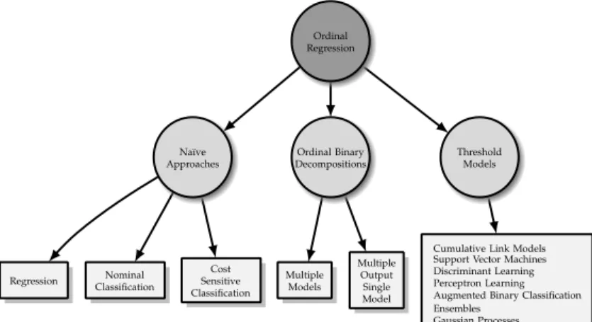
N ORDINAL REGRESSION TAXONOMYIn this section, a taxonomy of ordinal regression methods is proposed. With this purpose we firstly review what have been referred to asna¨ıve approaches, in the sense that the model is obtained by using other standard machine learning prediction algorithms (e.g. nominal classifica-tion or standard regression). Secondly,ordinal binary de-composition approachesare reviewed, the main idea being to decompose the ordinal problem into several binary ones, which are separately solved by multiple models or by one multiple-output model. The third group will
include the set of methods known as threshold models, which are based on the general idea of approximating a real value predictor and then dividing the real line into intervals. The taxonomy proposed is given in Fig. 1.
3.1 Na¨ıve approaches
Ordinal regression problems can be easily simplified into other standard problems, which generally involves making some assumptions. As will be later discussed, these methods can be very competitive given that, even though these assumptions may not hold, they inherit the performance of very well-tuned models.
3.1.1 Regression
One idea is to cast all the different labels{C1,C2, . . . ,CQ}
into real values {r1, r2, . . . , rQ} [51], whereri ∈R, and
then to apply standard regression techniques [2], [52], [53] (such as neural networks, support vector regres-sion...). Typically, the value of each label is related to its position in the ordinal scale, i.e.ri=i. For example, Kramer et al. [54] map the ordinal scale by assigning numerical values, applying a regression tree model and rounding the results for assigning the class when pre-dicting new values. They also evaluate the possibility of using the median, the mode, or the rounded mean of all the patterns in the leaves of the tree. The main problem with these approaches is that real values used for the labels may hinder the performance of the regression algorithms, and there is no principled way of deciding the value a label should have without prior information about the problem, since the distance between classes is unknown. Moreover, regression learners will be more sensitive to the representation of the label rather than its ordering [55]. A recent alternative is proposed in [56], where, instead of choosing arbitrary ordered values for the different labels, the variable is reconstructed by examining the different pairwise class distances.
3.1.2 Nominal classification
Ordinal classification problems are usually considered from a standard nominal perspective, and the order between classes is simply ignored. Some researchers routinely apply nominal response data analysis methods (yielding results invariant to the permutation of the categories) to both nominal and ordinal target variables alike because they are both categorical [57]. Nominal classification algorithms ignore the ordering of the labels, thus requiring more training data [55]. The Support Vector Machine paradigm (SVM) [58] is perhaps the most common kernel learning method for statistical pattern recognition. Beyond the application of the kernel trick to allow non-linear decision discriminants, and the slack-variables to avoid inseparability, relax the constraints and handle noisy data, the original binary SVM had to be reformulated to deal with multiclass problems [59].
Nominal Classification Ordinal Binary Decompositions Multiple Models Na¨ıve Approaches Regression Threshold Models
Cumulative Link Models Support Vector Machines Discriminant Learning Perceptron Learning Augmented Binary Classification Ensembles Gaussian Processes Multiple Output Single Model Cost Sensitive Classification Ordinal Regression
Fig. 1. Proposed taxonomy for ordinal regression meth-ods
TABLE 1
Example of different cost matrices for a five class classification problems, with class labels
y∈ Y ={C1,C2,C3,C4,C5}.
Zero-one Absolute cost Quadratic cost
0 1 1 1 1 1 0 1 1 1 1 1 0 1 1 1 1 1 0 1 1 1 1 1 0 0 1 2 3 4 1 0 1 2 3 2 1 0 1 2 3 2 1 0 1 4 3 2 1 0 0 1 4 9 16 1 0 1 4 9 4 1 0 1 4 9 4 1 0 1 16 9 4 1 0
Actual class labels are arranged in rows, while predicted class labels are arranged in columns.
3.1.3 Cost-sensitive classification
A more advanced method that can be considered in this group is cost-sensitive learning. Many real-world appli-cations of machine learning and data mining require the evaluation of the learned system with different costs for different types of misclassification errors [60]. This is the case with ordinal regression, although the exact costs for misclassification can not be always evaluated a priori. The cost of misclassifications can be forced to be different depending on the distance between real and predicted classes, in the ordinal scale. The work of Kotsiantis and Pintelas [61] considers cost-sensitive classification, by using absolute costs (i.e. the element cij of the cost matrix C is equal to the difference in the number of categories, cij =|i−j|). Different algo-rithms are shown to obtain better M AE values when cost matrices are used, without harming (in fact even improving) accuracy [61]. We include two cost matrices for a five class problem in Table 1, with the absolute cost matrix and the quadratic cost (cij = |i − j|2),
together with a zero-one cost matrix, which is the one assumed in nominal classification. Other possibilities are to choose asymmetric costs or non-convex two-Gaussian cost [41]. Again, the main problem is that, without a priori knowledge of the ordinal regression problem, it is not clear which cost matrix is more suitable.
TABLE 2
Binary decompositions for a5-class ordinal problem, with class labelsy∈ Y={C1,C2,C3,C4,C5}. Nominal decompositions OneVsAll OneVsOne +,−,−,−,− −,+,−,−,− −,−,+,−,− −,−,−,+,− −,−,−,−,+ −,−,−,−, , , , , , +, , , ,−,−,−, , , ,+, , ,+, , ,−,−, , ,+, , ,+, ,+, ,− , , ,+, , ,+, ,+,+ Ordinal decompositions
OrderedPartitions OneVsNext OneVsFollowers OneVsPrevious
−,−,−,− +,−,−,− +,+,−,− +,+,+,− +,+,+,+ −, , , +,−, , ,+,−, , ,+,− , , ,+ −, , , +,−, , +,+,−, +,+,+,− +,+,+,+ +,+,+,+ +,+,+,− +,+,−, +,−, , −, , ,
3.2 Ordinal binary decompositions
This group includes all those methods which are based on decomposing the ordinal target variable into several binary ones, which are then estimated by a single or multiple models. A summary of the decompositions is given in Table 2, where five classes are considered, each method generating a different decomposition matrix. Columns of the matrix correspond to the binary lems and rows to the role of each class for each subprob-lem. The symbol+is associated to the positive class and the symbol−to the negative one. If the class is not used in the specific binary subproblem, no symbol is included in the corresponding position. OneVsAll and OveVsOne
formulations are nominal classification methods (and should be listed as na¨ıve approaches), but they have been included in this table for comparison purposes. Note the high number of binary decompositions needed by
OneVsOne (in this case,10combinations).
Two main issues have to be taken into account when analysing the methods herein presented: 1) some of them are based on the idea of training a different model for each subproblem (multiple model approaches), while others learn one single model for all the subproblems; 2) apart from defining how to decompose the problem, it is important to define a rule for predicting new patterns, once the decision values are obtained. For the prediction phase, the corresponding binary codes of Table 2 can be considered as part of the error-correcting output codes (ECOC) framework [62], where the predicted class is the one closest to the code formed by all binary responses. Taking the first criterion into account, we have divided ordinal binary decomposition algorithms into multiple modeland multiple-output single modelapproaches. 3.2.1 Multiple model approaches
Ordinal information gives us the possibility of compar-ing the different labels. For a given rank q, a direct question can be the following, “is the label of pattern x greater than q?” [41]. This question is clearly a binary classification problem, so ordinal classification can be solved by considering each binary classification problem
independently and combining the binary outputs into a label, which is the approach followed by Frank and Hall in [63] (this decomposition is called OrderedPartitions in Table 2). In their work, Frank and Hall considered C4.5 as the binary classifier and the decision of the different binary classifiers were combined by using associated probabilitiespq =P(y≻ Cq|x), q= 1, . . . , Q−1:
P(y=C1|x)≈1−p1, P(y=CQ|x)≈pQ−1,
P(y=Cq|x)≈pq−1−pq, 2≤q≤Q−1.
Note that this approach may lead to negative probability estimates [64], given that binary classifiers are indepen-dently learned and nothing assures that pq−1 < pq.
When there is no need for proper probability estimations, prediction can be done by selecting the maximum.
In the work of Waegeman et al. [65], this framework is used but explicit weights over the patterns of each binary system are imposed, in such a way that errors on training objects are penalised proportionally to the ab-solute difference between their rank andq(the category examined). Additionally, labels for the test set are ob-tained by combining the estimated outcomesyq of all the Q−1binary classifiers. The interpretation of these binary outcomesyqi ∈ {+1,−1}, q = 1, . . . , Q−1, i = 1, . . . , N, intuitively leads toyi≻ Cq if yqi= +1. In this way, the rankkis assigned to patternxiso thatyqi=−1,∀q < k, and yqi = +1,∀q ≥ k. As stated by the authors, this strategy can result in ambiguities for some test patterns, and they should be solved by using similar techniques to those considered for nominal classification. A very similar scheme is proposed in [12], where the weights are obtained slightly differently, and different kernels are used for the different binary classification sub-problems. Other ordinal binary decompositions can be found in the literature. The cascade linear utility model [66] considersQ−1projections, in such a way that projection q separates classes C1∪. . .∪ CQ−q−1 from class CQ−q, i.e. one class is eliminated for each projection (this is the OneVsPrevious decomposition in Table 2). The pre-dictions are then combined by a union utility function. Finally, binary SVMs were also applied to ordinal re-gression [15], by making use of the ordinal pairwise partitioning approach [14]. This approach is composed of four different reformulations of the classical OneVsOne
andOneVsAllparadigms.OneVsNextconsiders that each binary classifierqseparates classCq from classCq+1, and
OneVsFollowers (which is similar to the OneVsPrevious
approach in [66] but in the opposite direction) constructs each binary classifierqfor the task of separating classCq from classesCq+1∪. . .∪ CQ. The prediction phase is then
approached by examining each binary classifier in order, so that, if a model predicts that the pattern is in the class which is isolated (not grouped with other classes), then this is the predicted class. This can be done in a forward manner or in a backward manner [15].
Finally, another possibility [67] is to derive a classifier for each class but separating the labels into groups
of three classes (instead of only two) for intermediate subtasks (labels lower than Cq, label Cq, and labels higher than Cq), or two classes for the extreme ones. The objective is to incorporate the order information in the subclassification tasks. Although the decomposition for intermediate classes is not binary but ternary, this approach has been included in this group because its motivation is similar to all the aforementioned.
3.2.2 Multiple-output single model approaches
Among non-parametric models, one appealing property of neural networks is that they can handle multiple responses in a seamless fashion [68]. Usually, as many output neurons as the number of target variables are included in the output layer and targets are presented to the network in the form of vectors ti, i = 1, . . . , N. When applied to nominal classification, the most usual approach is to consider a 1-of-Q coding scheme [53], i.e. ti = {ti1, . . . , tiQ}, tiq = 1 if xi corresponds to an example belonging to class Cq, and tiq = 0 (or tiq = −1), otherwise. In the ordinal regression framework, one can take the ordering information into account to design specific ordinal target coding schemes, which can improve the performance of the methods. Indeed, all the decompositions in Table 2 can be used to train neural networks, by taking each row as the code for the target class, ti, and a single model will be obtained for all related subproblems (considering that each output neuron is solving each subproblem). This can be done by assigning a value (+1, 0 or −1) to each of the different symbols (+ or −) in Table 2. For sigmoidal output neurons, a1is assigned for positive symbols (+) and a0 for negative ones (−). For hyperbolic functions, negative symbols are represented with a −1 and positive ones also with a 1. Those decompositions where a class is not involved should be treated as a “does not matter” condition where, whatever the output response, no error signal should be generated [69].
A generalisation of ordinal perceptron learning [70] in neural networks was proposed in [71]. The method is based on two main ideas: 1) the targets are coded using the OrderedPartitions approach; and 2) instead of using the softmax function [53] for the output nodes, a standard sigmoid function is imposed, and the category assigned to a pattern is equal to the index previous to that of the first output node whose value is higher than a predefined threshold T, or when no nodes are left. This method ignores inconsistencies (e.g. a sigmoid with value higher thanT after the index selected).
Extreme learning machines (ELMs) are single-layer feedforward neural networks, where the hidden layer does not need to be tuned given that corresponding weights are randomly assigned. ELMs have demon-strated good scalability and generalisation performance with a faster learning speed when compared to other models such as SVMs [72]. They have been adapted to ordinal regression [73], and one of the proposed ordinal ELMs also considers OrderedPartitions targets.
Additionally, multiple models are also trained using the
OneVsOneand theOrderedPartitionsapproaches. For the prediction phase, the loss-based decoding approach [62] is utilised, i.e. the chosen label is that which minimises the exponential loss, k = arg minq=1,...,Qd(Mq,y(x)), where Mq is the code associated to class q (q-th row of the coding matrix), y(x) is the vector of predic-tions, and d(Mq,y(x))is the exponential loss function, d(Mq,y(x)) =PQi=1exp (Mqi·yi(x)). The values of the vector y(x) are assumed to be in the [−1,+1] range, and those of Mq in the set{−1,0,+1}. The single ELM was found to obtain slightly better generalisation results and also to report the lowest computational time [73]. Other adaption of the ELM is found in [74], where an evolutionary algorithm is applied to optimise the different weights of the model by using a fitness function to impose the ordering restriction in model selection. A different approach is taken in [75], where the ordinal constraints are included into the weights connecting the hidden and output layers.
Costa [69] followed a probabilistic framework to pro-pose another neural network architecture able to exploit the ordinal nature of the data. The proposal is based on the joint prediction of constrained concurrent events, which can be turned into a classification task defined in a suitable space through a “partitive approach”. An appropriate entropic loss is derived for P(Y), i.e. the set of subsets of Y, where Y is a set of Q elementary events. A probability for each possible subset should be estimated, leading to a total of 2Q probabilities. However, depending on the classification problem, not all possibilities should be examined. For example, this is simplified for random variables taking values in finite or-dered sets (i.e. ordinal regression), as well as in the case of independent boolean random variables (i.e. nominal classification). To adapt neural networks to the ordinal case structure, targets were reformulated following the
OneVsFollowers approach and the prediction phase was accomplished by considering that, under its constrained entropic loss formulation, the output of theq-th output neuron estimates the probability thatqand q−1 events are both true. This methodology was further evaluated and compared in other works [64], [76], [77].
Although all these neural network approaches consist of a single model, they are trained independently in the sense that the output of the neurons do not depend on the other outputs (only on common nonlinear trans-formations of the inputs). That is the reason why we have included them into the category of ordinal binary decompositions.
These neural network models can be grouped under the term multitask learning [78] (MTL), which is a learn-ing paradigm that considers the case of simultaneously tackling several related tasks. Any of the different pro-posals in this field could be applied to train a single model for the different ordinal decompositions analysed in this section. Indeed, one of the existing proposals, MTL via conic programming [79], was validated in the
context of ordinal regression, showing promising results.
3.3 Threshold models
Often, in the ordinal regression paradigm, it is natural to assume that an unobserved continuous variable un-derlies the ordinal response variable. Such a variable is called a latent variable, and methods based on that assumption are known as threshold models, which are the most popular approaches for modelling ordinal and ranking problems [49]. These methodologies estimate:
• A functionf(x)that tries to predictthe values of the
latent variable, acting as a mapping function from feature space to the real one (similar to the ranking function to be learned by multipartite algorithms).
• A set of thresholds b= (b1, b2, . . . , bQ−1)∈RQ−1 to
represent intervals in the range off(x), which must satisfy the constraints b1≤b2≤. . .≤bQ−1.
Threshold models can be seen as an extension of na¨ıve regression models. The main difference between these two approaches is that the distances among the different classes are not defined a priori for threshold models, being estimated during the learning process. Although they are also related to (single-model) ordinal binary decomposition approaches, the main difference is that threshold models are based on one single projection
vector with multiple thresholds, one for each class.
3.3.1 Cumulative link models
Arising from a statistical background, the Proportional Odds Model (POM) is one of the first models specifically designed for ordinal regression [80], dated back to 1980. It is a member of a wider family of models recognised as Cumulative Link Models (CLMs) [81]. In order to extend binary logistic regression to ordinal regression, CLMs predict probabilities of groups of contiguous categories, taking the ordinal scale into account. In this way, cumu-lative probabilitiesP(y Cj|x)are estimated, which can be directly related to standard probabilities:
P(y Cq|x) =P(y =C1|x) +. . .+P(y=Cq|x),
P(y=Cq|x) =P(y Cq|x)−P(y Cq−1|x),
with q = 2, . . . , Q, and considering by definition that
P(y=C1|x) =P(y C1|x)and P(y CQ|x) = 1.
A decision rule f : X → Y is not fitted directly.
Instead, stochastic ordering of space X is satisfied by
the following general model form [28]:
g−1(P(y Cq|x)) =bq−wTx, q= 1, . . . , Q,
where g−1 : [0,1]→(−∞,+∞) is a monotonic function
often referred to as the inverse link function and bq is
the threshold defined for class Cq. This model is clearly
inspired by the latent variable motivation, considering thatf(x) =wTxis a linear transformation. Consider the
error of the model of the latent variable,f(x) =wTx+ǫ,
whereǫis the random component with zero expectation,
E[ǫ] = 0, distributed according to Fǫ. If a distribution
assumption Fǫ is made for ǫ, the cumulative model
is obtained by choosing the inverse distribution F−1
ǫ
as the inverse link function g−1. The most common
choice for the distribution of ǫ is the logistic function
(which is indeed the one selected for the POM [82]), although probit, complementary log, negative log-log or cauchit functions could also be used [81]. If the ordinal response is a coarsely measured latent
continu-ous variablef(x), labelCq in the training set is observed
if and only iff(x)∈[bq−1, bq], where the functionf and
b = (b0, b1, ..., bQ−1, bQ) are to be determined from the
data. It is assumed that b0 = −∞ and bQ = +∞, so
the real line, defined by f(x), x ∈ X, is divided into
Q consecutive intervals. Each region separated by two
consecutive biases corresponds to a category Cq. The
constraintsb1≤b2≤. . .≤bQ−1 ensure thatP(y Cq|x)
increases with q[83].
As will be seen, all the models in this section are inspired by the POM in the strategy assumed, obtaining a one-dimensional mapping function and dividing the real line into different ordered intervals. This mapping function can be used to obtain more information about the confidence of the predictions by relating it to its proximity to the biases. Additionally, the POM model
provides us with a solid probabilistic interpretation.The
distribution of ǫ is assumed to be the standard logistic function for the POM:
g−1(P(y Cq|x)) = ln P(y Cq|x) P(y≻ Cq|x) =bq−wTx, whereq= 1, . . . , Q−1,odds(y Cq|x) = exp(bq−wTx), so odds(y Cq|x) = P(yCq|x)
1−P(yCq|x). Therefore, the ratio of the odds for two pattens x0 andx1 are proportional:
odds(y Cq|x1)
odds(y Cq|x0)
= exp(−wT(x
1−x0)).
More flexible non-proportional alternatives have been
developed, one of them simply assuming differentwfor
each class (which is known as the generalised ordered logit model [84]). Another alternative applies the pro-portional odds assumption only to a subset of variables
(partial proportional odds [85]). Moreover, Tutz [86]
presented a general framework for parametric models that extends generalised additive models to incorporate nonparametric parts.
Apart from assuming proportional odds, linear CLMs
are rather inflexible since the decision functions are
always linear hyperplanes, this generally affecting the performance of the model (as analysed in the experi-mental section of this work). A non-linear version of the POM model was proposed in [18], [83] by simply setting the projectionf(x)to be the output of a neural network. The probabilistic interpretation of CLMs can be used to apply a maximum likelihood maximisation for setting the network parameters. Gradient descent techniques with proper constraints for the biases serve this purpose. This non-linear generalisation of the POM model based on neural networks was considered in [87], where an
evolutionary algorithm was applied to optimise all the parameters considered. Linear ordinal logistic regression was combined with nonlinear kernel machines using primal-dual relations from Nystrom sampling [88]. How-ever, to make the computation of the model feasible, a sub-sample from the data had to be selected, which limits the applicability to those cases where there is a reasonable way to do this [88].
An interesting alternative to CLMs is the so-called ordistic model presented in [89]. The work presents two threshold-based constructions which can be used to generalise loss functions for binary labels, such as the logistic and hinge loss, and another generalisation of the logistic loss based on a probabilistic model for ordered labels. Both constructions are based on including Q−1thresholds partitioning the real line toQsegments, but they differ in how predictors outside the “correct” segment (or too close to its edges) are penalised. The immediate-threshold construction only penalises the vio-lations of the two thresholds limiting this segment, while the all-threshold one considers all of them.
3.3.2 Support vector machines
Because of their good generalisation performance, SVM models are maybe the most widely applied ones to ordinal regression, their structure being easily adapted to that of threshold models. The proposal of Herbrich et al. [28], [90] is the first SVM based algorithm, where they consider a pairwise approach by deriving a new dataset made up of all possible difference vectors xd
ij =xi−xj andyij = sign (O(yi)− O(yj)), withyi, yj∈ {C1, . . . ,CQ}.
In contrast, all the SVM pointwise approaches share the common objective of seeking Q−1 parallel discrimi-nant hyperplanes, all of them represented by a common vector w and the scalars biases b1 ≤ . . . ≤ bQ−1 to
properly separate training data into ordered classes. In this sense, several methodologies for the computation of w and {b1, . . . , bQ−1} can be considered. The work of
Shashua and Levin [91] introduced two first methods: the maximisation of the margin between the closest neighbouring classes and the maximisation of the sum of margins between classes. Both approaches present two main problems [64]: the model is incompletely speci-fied, because the thresholds are not uniquely defined, and they may not be properly ordered at the optimal solution, since the inequalityb1≤b2≤. . .≤bQ−1 is not
included in the formulation.
Consequently, Chu and Keerthi [29], [92] proposed two different reformulations for the same idea, solving the problem of unordered thresholds at the solution. On the one hand, they imposed explicit constraints on the optimisation problem, only considering adjacent la-bels for threshold determination (Support Vector Ordinal Regression with Explicit Constraints, SVOREX). On the other hand, patterns in all the categories were allowed to contribute errors for each hyperplane (SVOR with Implicit Constraints, SVORIM), which, as they prove [29], leads to automatically satisfied constraints in the
optimal solution (see Lemma 1 of [29]). Let Nq be the
number of patterns of class Cq, and let xqi be those
patternsxwhich class label isCq. The SVORIM learning
problem is defined as follows:
min w,b,ξ,ξ∗ 1 2||w||+C Q−1 X q=1 q X j=1 Nq X i=1 ξjiq + Q X j=q+1 Nq X i=1 ξ∗jiq ,
subject to the constraints:
w·xji −bq ≤ −1 +ξqji, ξ q ji≥0, j∈ {1, . . . , q}, w·xji −bq ≥+1−ξji∗q, ξ ∗q ji ≥0, j∈ {q+ 1, . . . , Q}, where i ∈ {1, . . . , Nq}, b ∈ RQ−1, ξqji and ξ ∗q ji are the
slacks for the q-th parallel hyperplane (defined for the
left and right part of the hyperplanes, respectively). The first group of constraints is focused on the left part
of the j-th hyperplane (classes with q ≤ j), while the
second one is focused on the right part (classes with
q > j).They empirically found that SVOREX performed better in terms of accuracy (with a more local behaviour), and SVORIM preceded in terms of absolute deviations in number of classes or M AE (with a more global behaviour), and this is justified theoretically based on the loss minimised for each method. The framework of reduction [41] also explains this from the point of view of the cost matrices selected. Our results seem to agree with these conclusions for discretised regression datasets, but the differences are not so clear for real ordinal regression ones. Generalisation properties for some ordinal regression algorithms, including SVOR, were further studied in [93].
In [94], the errors of an ordinal SVM classifier are studied separately depending on whether they corre-spond to upgrading errors (predicted label higher than the actual one) or downgrading ones (the predicted label being lower than the actual one). Authors address the two-objective problem of finding a classifier maximising simultaneously the two margins, and they show that the whole set of Pareto-optimal solutions can be obtained by solving a quadratic optimisation problem.
Some recent works focused on solving the bottle-neck of these SVM proposals, which is usually the high computational complexity to handle larger datasets. Concerning this topic, two different proposals can be distinguished: block-quantised support vector ordinal regression [95] and ordinal-class core vector machines [96]. The former is based on performing kernelk-means and applying SVOR in the cluster representatives, on the idea of approximating the kernel matrixK byK˜ which will be composed of k2 constant blocks, in such a way
that the problem scales with the number of clusters, in-stead of the dataset size. The latter is an extension of core vector machines [97] in the ordinal regression setting. Finally, an incremental version of SVOR algorithms is proposed in [98].
3.3.3 Discriminant learning
Discriminant learning has also been reformulated to tackle ordinal regression [31]. Discriminant analysis is usually not considered as a classification technique by itself, but rather as a supervised dimensionality reduc-tion. Nonetheless, it is widely used for that purpose, since, as a projection method, the definition of thresholds can be used to discriminate the classes. In general, to allow the computation of the optimal projection for the data, this algorithm analyses two main objectives: the maximisation of the between-class distance, and the min-imisation of the within-class distance, by using variance-covariance matrices and the Rayleigh coefficient. In order to reformulate the algorithm for ordinal regression, an ordering constraint over contiguous classes is imposed on the averages of projected patterns of each class, which leads the algorithm to order projected patterns according to their label. This will preserve the ordinal information and avoid some serious ordinal misclassification errors. The original optimisation problem is transformed and extended with a penalty term (C):
minJ(w, ρ) =wTSww−Cρ,
subject towT(mq+1−mq)≥ρ, wheremq =Nq1 PNqi=1xi,
Sw is the within-class scatter matrix and ρ represents
the minimum difference of the projected means between consecutive classes (if ρ > 0, the projected means are correctly ranked). This methodology is known as Kernel Discriminant Learning for Ordinal Regression (KDLOR) [31] and it has been used in some later works [9], [99]. In [100], the KDLOR model is extended by trying to learn multiple orthogonal projections, which are then combined into a final decision function.
The method was extended in [101], [102] based on the idea of preserving the intrinsic geometry of the data in the embedded non-linear structure, i.e. in the induced high-dimensional feature space, via kernel map-ping. This consideration is the basis of manifold learning [53], and the algorithms mentioned construct a neigh-bourhood graph (which takes the ordinal nature of the dataset into account) which is afterwards used to derive the Laplacian matrix and obtain a projection which considers the underlying manifold of the data. A related method is proposed in [103], where several different projections are iteratively derived.
3.3.4 Perceptron learning
PRank [104] is a perceptron online learning algorithm with the structure of threshold models. It was then ex-tended by approximating the Bayes point, what provides good performance for generalisation [55].
3.3.5 Augmented binary classification
Although the approaches in Subsection 3.2 are simple to implement, their generalisation performance cannot be analysed easily. The two algorithms included in this
TABLE 3
Extended binary transformation for three given patterns
(x1, y1=C1),(x2, y2=C2),(x3, y3=C3), the identity coding matrix and the quadratic cost matrix.
x(q) i i q wi,q x mq yi(q) 1 1 2· |0−1|= 2 x1 {1,0} 2J1<1K−1 =−1 1 2 2· |1−4|= 6 x1 {0,1} 2J2<1K−1 =−1 2 1 2· |1−0|= 2 x2 {1,0} 2J1<2K−1 = +1 2 2 2· |0−1|= 2 x2 {0,1} 2J2<2K−1 =−1 3 1 2· |4−1|= 6 x3 {1,0} 2J1<3K−1 = +1 3 2 2· |1−0|= 2 x3 {0,1} 2J2<3K−1 = +1
subsection work differently, and, as later analysed, the models derived are equivalent to threshold models.
A reduction framework can be found in the works of Lin and Li [41], [105], where ordinal regression is reduced to binary classification by applying three steps:
1) A coding matrix M is used to represent the class
being examined. Given a coding matrix M of
(Q−1)rows, input patterns(xi, yi)are transformed into extended binary patterns by replicating them, (x(iq), yi(q)), with:
xi(q)= (xi,mq), yi(q)= 2Jq <O(yi)K−1, where q = 1, . . . , Q−1, mq is the q-th row of M and J·K is a Boolean test which is 1 if the inner condition is true, and0otherwise.Q−1 replicates of each pattern are generated with weights:
wi,q= (Q−1)· |CO(yi),q−CO(yi),q+1|,
where i = 1, . . . , N, C is a V-shaped cost ma-trix (i.e. CO(yi),q−1 ≥ CO(yi),q, if q ≤ O(yi), and
CO(yi),q ≤ CO(yi),q+1, if q ≥ O(yi)). The cost
matrix must be defined a priori. An example of this transformation is given in Table 3. As can be seen, the final extended pattern represents the
question “Is the rank ofxgreater thanq?” [41]. The
weights measure the importance of the pattern for the binary classifier, and they are also used for the theoretical analysis.
2) A single binary classifier with confidence outputs, f(x,mk), is trained for the newweightedextended patterns, aiming at a low weighted 0/1 loss. 3) A classification rule like the following is used to
construct a final prediction for new patterns: r(x) = 1 +
Q−1
X
q=1
Jf(x,mq)>0K. (1) All the binary classification problems are solved jointly by computing a single binary classifier. The most striking characteristic of this algorithm is that it unifies many existing ordinal regression algorithms [41], such as the perceptron ones [104], kernel ranking [36], AdaBoost.OR [106], ORBoost-LR and ORBoost-All thresholded ensem-ble models [107], CLM [81] or several ordinal SVM
proposals (oSVM [64], SVORIM and SVOREX [29]). Moreover, it is important to highlight the theoretical guarantees provided by the framework, including the derived cost and regret bounds and the proof of equiv-alence between ordinal regression and binary classifi-cation. An extension of this reduction framework was proposed in [108], where ordinal regression is proved to be equivalent to a regular multiclass classification whose distribution is changed. This extension is free of the following restrictions: target functions should be rank-monotonic; and rows of loss matrix are convex.
The data replication method of Cardoso et al. [64] (whose previous linear version appeared in [10]) is a very similar framework, except that it essentially con-siders the absolute cost, consequently being less flexible. However, for ordinal regression, increasing the error with the absolute difference between the predicted and estimated labels is a natural choice in the absence of any other information [18]. An advantage of the framework of data replication is that it includes a parameterswhich limits the number of adjacent classes considered, in such a way that the replicate q is constructed by using the q−sclasses to its ’left’ and theq+sclasses to its ’right’ [64]. This parameter s∈ {1, ..., Q−1} plays the role of controlling the increase of data points.
It is worth mentioning that augmented binary classifi-cation models and threshold models are closely related, and that is the reason why they have been included in this section. The extended patterns only differ in the
new variables introduced by the coding matrix M. The
original version of the dataset is replicated in different subspaces, with different values for the new variables. By obtaining the intersection of the binary hyperplane in the extended dataset with each of the subspace replicas we derive parallel boundaries in the original dataset [64], with a single projection vector and multiple thresholds.
In fact, SVORIM and reduction to SVM is known to be not so different in formulation [103]. The model of Mathieson [18] (threshold model) is equivalent to the one proposed in [64] (oNN, an augmented binary classification model) if the activation function of the output node is set to the logsig function and the model is trained to predict the posterior probabilities when fed with the original input variables and the variables generated by the data replication method. The predicted thresholds would be the weights of the connection of the addedQ−2 components.Finally, augmented binary classification and ordinal binary decomposition are not disjoint categories. The former class of models do not restrict consistency of binary classifiers, making use of a “voting” of the binary classifiers (see Eq. 1 of [105]). Moreover, all the ordinal decompositions in Table 2 can be viewed as a special case of “cost-sensitive ordinal classification” via augmented binary classification [41].
3.3.6 Ensembles
From a different perspective, the confidence of a binary classifier can be regarded as an ordering preference.
RankBoost [109] is a boosting algorithm that constructs an ensemble of those confidence functions to form a better ordering preference. Some efforts were made to apply a similar idea for ordinal regression problems, deriving into Ordinal Regression Boosting (ORBoost) [107]. The corresponding thresholded-ensemble models inherit the good properties of ensembles, including more stable predictions and sufficient power for approximat-ing complicated target functions [110]. The model is composed of confidence functions, and their weighted linear combination is used as the projectionf(x).A set of thresholds for this projection is also included in the model and iteratively updated with the rest of
parame-ters.Following a similar approach to [89], large margin
bounds of the classification error and the absolute error are derived, from which two algorithms are presented: ORBoost with all margins and ORBoost with left-right margins [107]. Two alternative thresholded-ensemble al-gorithms are presented in [111], both generating an ensemble of ordinal decision rules based on forward stagewise additive modelling.
With a different perspective, the well-known Ad-aBoost algorithm was recently extended to improve any base ordinal regression algorithm [106]. The extension, AdaBoost.OR, proved to inherit the good properties of AdaBoost, improving both the training and test perfor-mances of existing ordinal classifiers. Another ordinal re-gression version of AdaBoost is proposed in [112], while in this case the adaption is based on considering a cost matrix both in pattern weighting and error updating.
The framework of negative correlation learning (where the ensemble members are learnt in such a way that the correlation between their responses is minimised) was used in the context of ordinal regression [17], [113] by calculating the correlation between the latent variable estimations or, alternatively, between the probabilities obtained by the ensemble members.
3.3.7 Gaussian processes
All the previous threshold models can be considered discriminative models in the sense that they estimate directly the posteriorP(y|x), or learn a function to map the input x to class labels. On the contrary, generative models learn a model of the joint probabilityP(x, y)of input patternsxand labely, and make the prediction by a Bayesian framework to estimateP(y|x).
Gaussian Processes for Ordinal Regression (GPOR) [30] models the latent variablef(x)using Gaussian Pro-cesses, to estimate then all the parameters by means of a Bayesian framework. The values of the latent function {f(xi)}are assumed to be the given by random variables indexed by their input vectors in a zero-mean Gaussian process. Mercer kernel functions approximate the covari-ance between the functions of two input vectors.Finally, the thresholds are included in the model to divide the latent variable in consecutive intervals, and they are optimised together with the rest of parameters, using
the latent function f, the joint probability of observing the ordinal variables is P(D|f) =QNi=1P(yi|f(xi)), and the Bayes theorem is applied to write the posterior prob-abilityP(f|D) = 1
P(D)
QN
i=1P(yi|f(xi))P(f). A Gaussian
noise with zero mean and unknown variance σ2 is
as-sumed for the latent functions. The normalisation factor P(D), more exactly P(D|θ), is known as the evidence
for the vector of hyperparameters θ and is estimated
in the paper by two different approaches: a Maximum a Posteriori approach with Laplace approximation and an Expectation Propagation with variational methods. A more general GPOR was then proposed to tackle multi-class multi-classification problems but with a free structure of preferences over the labels [114]. A probabilistic sparse kernel model was proposed for ordinal regression in [115], where a Bayesian treatment was also employed to train the model. A prior over the weights governed by a set of hyperparameters was imposed, inspired by the well-known relevance vector machine. Srijith et al. have proposed a probabilistic least squares version of GPOR [116], two different sparse versions [117] and a semi-supervised version [118].
3.4 Other approaches and problem formulations
This subsection includes some methods that are difficult to consider in the previous groups. For example, an alternative methodology is proposed by da Costa et al. [76], [77] for training ordinal regression models. The main assumption of their proposal is that the random variable class associated with a given pattern should follow a unimodal distribution. For this purpose, they provide two possible implementations: a parametric one, where a specific discrete distribution is assumed and the associated free parameters are estimated by a neural network; and a non-parametric one, where no distribu-tion is assumed but the error funcdistribu-tion is modified to avoid errors from distant classes. The same idea was then applied to SVMs in [119] by solving an ordinal problem through a single optimisation process (the all-at-once strategy).
In [120], both decision trees and nearest neighbour (NN) classifiers are applied to ordinal regression prob-lems by introducing the notion of consistency: a small change in the input data should not lead to a ’big jump’ in the output decision, i.e. adjacent decision regions should have equal or consecutive labels. This rationale was used as a post-processing mechanism of a standard decision tree and as a pre- or post- processing step for the NN method. An improvement was presented in [121] to reduce the over-regularised decision region artifact by using ensemble learning techniques.
Two ordinal learning vector quantisation schemes, with metric learning, specifically designed for classifying data items into ordered classes, are introduced in [122], [123]. The methods use the order information during training, both in the selection of the prototypes and for determining the way they are updated.
Different prediction methods as a function of the error measure to be minimised are presented in [124]. The pa-per discusses the fact that the Bayes optimal decision for a classifier which return probability estimates is different depending on the loss function considered for the errors. In this way, for the maximisation of the accuracy one should consider the mode (or maximum probability), but the median of the probability distribution is the optimal decision when minimising theM AE in ordinal regression problems.
4
E
XPERIMENTAL STUDY4.1 Experimental design
In this subsection, the experiments are clearly specified, including the datasets and algorithms considered, the parameters to optimise, the performance measures and the statistical tests used for assessing the differences. 4.1.1 Datasets selected
The most widely used dataset repository is the one pro-vided by Chu et al. [30], including different regression benchmark datasets. These datasets are not real ordinal classification problems but regression ones, which are turned into ordinal classification by discretising the tar-get intoQdifferent bins with equal frequency. It is clear that these datasets do not exhibit some characteristics of typical complex classification tasks, such as class imbal-ance, given that all classes are assigned the same number of patterns. However, we find interesting to check how the algorithms perform in this more controlled environ-ment and to compare the conclusions obtained.
Table 4 shows the characteristics of the 41 datasets, including the number of patterns, attributes and classes, and also the number of patterns per class. The real ordinal classification datasets were extracted from bench-mark repositories1 (UCI [125] and mldata.org[126]),
and the regression ones were obtained from the website of W. Chu2. For the discretised datasets, we considered
Q = 5 and Q = 10 bins to evaluate the response of the classifiers to the increase in the complexity of the problem. The synthetic toy dataset was generated as proposed in [77] with 300 patterns. All nominal at-tributes were transformed into as many binary atat-tributes as the number of categories, and all the datasets were properly standardised.
4.1.2 Algorithms selected
We have selected some representatives of the different families included in the proposed taxonomy (see Table 5). It is important to note that na¨ıve approaches and ordinal binary decompositions can be applied using almost any base binary classifier or regressor. In our ex-periments, we have selected in those cases SVMs, given
1. We would like to note that many of these datasets have been previously considered in machine learning literature, but ignoring the ordering information.
TABLE 4
Characteristics of the benchmark datasets Discretised regression datasets
Dataset #Pat. #Attr. #Classes Class distribution
pyrim5 (P5) 74 27 5 ≈15per class
machine5 (M5) 209 7 5 ≈42per class housing5 (H5) 506 14 5 ≈101per class
stock5 (S5) 700 9 5 140per class
abalone5 (A5) 4177 11 5 ≈836per class bank5 (B5) 8192 8 5 ≈1639per class bank5’ (BB5) 8192 32 5 ≈1639per class computer5 (C5) 8192 12 5 ≈1639per class computer5’ (CC5) 8192 21 5 ≈1639per class cal.housing5 (CH5) 20640 8 5 4128per class
census5 (CE5) 22784 8 5 ≈4557per class census5’ (CEE5) 22784 16 5 ≈4557per class pyrim10 (P10) 74 27 10 ≈8per class machine10 (M10) 209 7 10 ≈21per class
housing10 (H10) 506 14 10 ≈51per class stock10 (S10) 700 9 10 70per class abalone10 (A10) 4177 11 10 ≈418per class
bank10 (B10) 8192 8 10 ≈820per class bank10’ (BB10) 8192 32 10 ≈820per class computer10 (C10) 8192 12 10 ≈820per class computer10’ (CC10) 8192 21 10 ≈820per class cal.housing (CH10) 20640 8 10 2064per class
census10 (CE10) 22784 8 10 ≈2279per class census10’ (CEE10) 22784 16 10 ≈2279per class
Real ordinal regression datasets
Dataset #Pat. #Attr. #Classes Class distribution contact-lenses (CL) 24 6 3 (15,5,4) pasture (PA) 36 25 3 (12,12,12) squash-stored (SS) 52 51 3 (23,21,8) squash-unstored (SU) 52 52 3 (24,24,4) tae (TA) 151 54 3 (49,50,52) newthyroid (NT) 215 5 3 (30,150,35) balance-scale (BS) 625 4 3 (288,49,288) SWD (SW) 1000 10 4 (32,352,399,217) car (CA) 1728 21 4 (1210,384,69,65) bondrate (BO) 57 37 5 (6,33,12,5,1) toy (TO) 300 2 5 (35,87,79,68,31) eucalyptus (EU) 736 91 5 (180,107,130,214,105) LEV (LE) 1000 4 5 (93,280,403,197,27) automobile (AU) 205 71 6 (3,22,67,54,32,27) winequality-red (WR) 1599 11 6 (10,53,681,638,199,18) ESL (ES) 488 4 9 (2,12,38,100, 116,135,62,19,4) ERA (ER) 1000 4 9 (92,142,181,172, 158,118,88,31,18)
that they are suggested by many of the authors of the dif-ferent works analysed. Starting with na¨ıve approaches, the following methods were considered: 1) C-Support Vector Classifier (C-SVC) withOneVsOne and OneVsAll
decompositions (SVC1V1 and SVC1VA), because they are the two main approaches when applying SVM to multiclass problems [59]. Although these methods con-sider binary decompositions, they have been included in the nominal classification group, given that they do not take the class order into account. 2) Support Vector Regression (SVR) applied to a modified dataset where the target variableY ={C1,C2, . . . ,CQ}is mapped to the
real values{0,1/(Q−1),2/(Q−1), . . . ,1}. The concrete regression model considered is the ǫ-SVR [52]. 3) Cost-Sensitive SVC (CSSVC), which is a C-SVC [59] with the OneVsAll decomposition, where absolute costs are included as different weights [127] for the negative class of each decomposition.
Regarding the ordinal binary decompositions, the methods considered are the following: 1) The Ordered-Partitionsdecomposition was applied to theC-SVC
clas-TABLE 5
Different algorithms considered for the experiments Abbr. Short description
Na¨ıve approaches
SVC1V1 Support Vector Classifier withOneVsOne[59] SVC1VA Support Vector Classifier withOneVsAll[59] SVR Support Vector Machines for regression [52] CSSVC Cost-Sensitive Support Vector Classifier (CSSVC) [59]
Ordinal Binary decompositions
SVMOP Support Vector Machines withOrderedPartitions[63], [65] NNOP Neural Network withOrderedPartitions[71]
ELMOP Extreme Learning Machine withOrderedPartitions[73]
Threshold models
POM Proportional Odds Model [80]
NNPOM Neural Network based on Proportional Odd Model [18] SVOREX Support Vector Ordinal Regression with Explicit Constraints [29] SVORIM Support Vector Ordinal Regression with Implicit Constraints [29]
SVORLin SVORIM using a linear kernel [29]
KDLOR Kernel Discriminant Learning for Ordinal Regression [31] GPOR Gaussian Processes for Ordinal Regression [30] REDSVM Reduction applied to Support Vector Machines [41] ORBALL Ordinal Regression Boosting with All margins [107]
sification algorithm (SVMOP), but including different weights, as proposed by Waegeman et al. [65]. However, given the problem of possible ambiguities recognised by the authors, probability estimates are obtained following the method presented in [128]. Then, the fusion of proba-bilities of Eq. (1) is performed [63]. 2) The neural network model proposed in [71] (NNOP). This model considers theOrderedPartitionscoding scheme for the labels and a rule for decisions based on the first node whose output is higher than a predefined threshold (T = 0.5, in our experiments). We consider then the mean square error function over the outputs and the iRProp+ algorithm [129] to optimise the parameters. 3) Finally, the single model ordinal ELM presented in [73] (ELMOP).
The threshold models considered are the following: 1) The POM [82], with thelogitlink function (the most pop-ular one). 2) A neural network approach based on the POM (NNPOM), similar to the one proposed by Math-ieson [18]. The cross entropy function is optimised by the iRProp+ algorithm [129]. Threshold constraints are satis-fied by substituting the set of parameters{b1, b2, . . . , bQ}
by {α1, α1+α22, . . . , α1+α22+. . .+αQ2}, which allows unconstrained optimisation of {α1, . . . , αQ}. 3) Ordinal
support vector formulations of Chu and Keerthi [29], including both explicitly and implicitly constrained alter-natives (SVOREX and SVORIM).We have also included a linear version of the SVORIM method (considering the linear kernel instead of the Gaussian one) to check how the kernel trick affects the final performance (SVORLin).
4) KDLOR algorithm presented in [31]. 5) The GPOR method [30] including automatic relevance determina-tion, as proposed by the authors. 6) The reduction from ordinal regression to binary SVM classifiers was also considered (REDSVM). The configuration used was the identity coding matrix, the absolute cost matrix and the standard binary soft-margin SVM, as proposed in [41]. 7) Finally, the ORBoost method with all margins [107] (OR-BALL). As proposed by the authors, the total number of ensemble members is set to T = 2000, and normalised