Internet Appendix for
Firm Level Productivity, Risk, and Return
Ay¸se ·Imrohoro¼glu ¸Selale Tüzely
July 2013
Abstract
This Internet Appendix presents material that is supplemental to the main analysis and tables in “Firm Level Productivity, Risk, and Return.”We supplement the empirical analysis in the paper with details on the measurement of TFP, detailed description of data, additional properties of TFP, and empirical robustness checks. We supplement the theoretical analysis with a …gure to illustrate the model mechanism and details of our numerical solution method.
Department of Finance and Business Economics, Marshall School of Business, University of Southern Cali-fornia, Los Angeles, CA 90089-1427. E-mail: [email protected]
yDepartment of Finance and Business Economics, Marshall School of Business, University of Southern
1
Measuring TFP
The main contributions to measuring …rm level TFP are by Olley and Pakes (1996) and Levin-sohn and Petrin (2003).1 The key di¤erence between the two methods is that Olley and Pakes (1996) use investment whereas Levinsohn and Petrin (2003) use materials used in production as a proxy for TFP. Since data on investment is readily available and often non-zero at the …rm level but data on materials is not, we follow Olley and Pakes (1996) to estimate …rm level productivities.
In our benchmark case, we estimate the production function based on labor and physical capital as inputs. The production technology is given by yit = F(lit; kit; !it) where yit is log
output for …rm i in period t. lit; kit are log values of labor and capital of the …rm. !it is the
productivity, and itis an error term not known by the …rm or the econometrician. Speci…cally:
yit= 0+ kkit+ llit+!it+ it: (1)
Olley and Pakes assume that productivity,!it;is observed by the …rm before the …rm makes
some of its factor input decisions, which gives rise to the simultaneity problem. Labor,lit;is the
only variable input, i.e., its value can be a¤ected by current productivity, !it:The other input,
kit; is a …xed input at time t; and its value is only a¤ected by the conditional distribution of
!itat time t 1. Consequently,!it is a state variable that a¤ects …rms’decision making where
…rms that observe a positive productivity shock in period twill invest more in capital,iit;and
hire more labor,lit;in that period. The solution to the …rm’s optimization problem results in
the equations foriit:
iit=i(!it; kit) (2)
where both iand j are strictly increasing in !: The inversion of the equations yield:
1Both approaches o¤er advantages over more traditional estimation techniques such as OLS. The static OLS
production function estimates reveal that within …rm residuals, which are the productivity estimates in that setting, are serially correlated. The simultaneity bias arises if the …rm’s factor input decision is in‡uenced by the TFP that is observed by the …rm. This means that the regressors and the error term in an OLS regression are correlated. The selection bias in the OLS regressions arises due to …rms exiting the sample used in estimating the production function parameters. If the exit probability is correlated with productivity, not accounting for the selection issue may bias the parameter estimates.
!it=h(iit; kit)
whereh is strictly increasing iniit.
De…ne:
it = 0+ kkit+h(iit; kit): (3)
Using equations (1) and (3), we can obtain
yit= llit+ it+ it (4)
where we approximate itwith a second order polynomial series in capital and investment.2 This …rst stage estimation results in an estimate for bl that controls for the simultaneity problem. In the second stage, consider the expectation of yi;t+1 blli;t+1 on information at time t and survival of the …rm:
Et yi;t+1 blli;t+1 = o+ kki;t+1+Et(!it+1j!it; survival) (5)
= o+ kki;t+1+g(!it;Pbsurvival;t)
wherePbsurvival;t denotes the probability of …rm survival from timetto time t+ 1. The survival
probability is estimated via a probit of a survival indicator variable on a polynomial expression containing capital and investment. We …t the following equation by nonlinear least squares:
yi;t+1 blli;t+1= kki;t+1+ !it+ Pbsurvival;t+ i;t+1 (6)
where!itis given by!it= it 0 kkit and is assumed to follow an AR(1) process.3 At the
end of this stage, bl and bk are estimated.
Finally, productivity is measured by:
Pit= exp(yit bo bllit bkkit): (7)
Since our data set covers di¤erent industries with di¤erent market structures and factor 2Approximating with a higher order polynomial instead does not signi…cantly change the results.
3
prices, we estimate equation (4) with industry speci…c time dummies and then subtract them from the left hand side of equation (5). Hence, our …rm level TFPs are free of the e¤ect of industry or aggregate TFP in any given year.4 Our use of industry speci…c time dummies and price de‡ators for investment remove the impact of possible embodied technological progress as modeled in Greenwood, Hercowitz, and Krusell (1997 and 2000) and Fernández-Villaverde and Rubio-Ramírez (2007).
2
Data
The main data source for …rm level productivity estimation is Compustat. We use the Compu-stat fundamental annual data from 1962 to 2009. We delete observations of …nancial …rms (SIC classi…cation between 6000 and 6999) and regulated …rms (SIC classi…cation between 4900 and 4999).5 Our sample for production function estimation is comprised of all remaining …rms in Compustat that have positive data on sales, total assets, number of employees, gross property, plant, and equipment, depreciation, accumulated depreciation, and capital expenditures. The sample period starts in 1962. The sample is an unbalanced panel with approximately 12,750 distinct …rms; the total number of …rm-year observations is approximately 128,000.6
The key variables for estimating the …rm level productivity in our benchmark case are the …rm level value added, employment, and physical capital.7 Firm level data is supplemented
with price index for Gross Domestic Product as de‡ator for the value added and price index for private …xed investment as de‡ator for investment and capital, both from the Bureau of Economic Analysis, and national average wage index from the Social Security Administration.
4
In another speci…cation, we compute …rm level TFPs without using industry dummies in our …rst stage estimation. We analyze the industry adjusted TFPs of …rms, which are the log TFPs in excess of their industry averages. The stylized facts generated from that framework are both qualitatively and quantitatively very similar to our results even though the production function estimates for labor and capital are somewhat di¤erent.
5We exclude …nancial …rms and regulated …rms since it is standard to do so in this literature. Keeping these
…rms in the sample does not change the results in any material way. The production function estimates for the …nancial …rms are quite similar to the production function estimates for the non-…nancial …rms.
6
At this stage, we do not require the …rms to be in the CRSP database. Hence, our sample size gets somewhat smaller later when we merge our dataset with CRSP data.
7Firms use many inputs in their production, such as raw materials, labor, di¤erent types of capital, energy,
etc. In our speci…cation, we focus on labor and physical capital as the main inputs. Consequently, …rm’s value added is de…ned as the gross output net of expenditures on materials as well as the other expensed items such as advertisement, R&D expenditures, and rental expenses. Hence, our value added variable contains the contribution of labor and owned physical capital of the …rm only.
Value added (yit) is computed as Sales - Materials, de‡ated by the GDP price de‡ator.8
Sales is net sales from Compustat (SALE).9 Materials is measured as Total expenses minus Labor expenses. Total expenses is approximated as [Sales - Operating Income Before Depreci-ation and AmortizDepreci-ation (Compustat (OIBDP))]. Labor expenses is calculated by multiplying the number of employees from Compustat (EMP) by average wages from the Social Security Administration).10 The stock of labor(lit)is measured by the number of employees from
Com-pustat (EMP). These steps lead to our value added de…nition that is proxied by Operating Income Before Depreciation and Amortization+labor expenses.
Capital stock (kit) is given by gross property, plant, and equipment (PPEGT) from
Com-pustat, de‡ated by the price de‡ator for investment following the methods of Hall (1990) and Brynjolfsson & Hitt (2003).11 Since investment is made at various times in the past, we need to calculate the average age of capital at every year for each company and apply the appropriate de‡ator (assuming that investment is made all at once in year [current year - age]). Average age of capital stock is calculated by dividing accumulated depreciation (Gross PPE - Net PPE, from Compustat (DPACT)) by current depreciation, from Compustat (DP). Age is further smoothed by taking a 3-year moving average.12 The resulting capital stock is lagged by one period to measure the available capital stock at the beginning of the period.13
The Longitudinal Research Database (LRD), a large panel data set of U.S. manufacturing 8Measures of productivity based on …rm revenues typically confound idiosyncratic demand and factor price
e¤ects with di¤erences in e¢ ciencies. Foster, Haltiwagner, and Syverson (2008) show that demand factors can be important in understanding industry dynamics and reallocation. Measures of productivity that incorporate demand factors require data on producers’physical outputs as well as product prices, which are not available at the …rm level. However, they also show that revenue based productivity measures, such as the one used in this study, are highly correlated with their physical productivity.
9
Net sales are equal to gross sales minus cash discounts, returned sales, etc.
1 0Compustat also has a data item called sta¤ expense (XLR), which is sparsely populated. Comparing our
labor expense series with the sta¤ expense data available at Compustat reveals that our approximation yields a relatively correct and unbiased estimate of labor expenses.
1 1
Hulten (1990) discusses many complications related to the measurement of capital. The principal options are to look for a direct estimate of the capital stock, K, or to adjust book values for in‡ation, mergers, and accounting procedures; or to use the perpetual inventory method to construct the capital stock from data on investments. There are problems associated with either method, and most of the time, the choice between these methods is dictated by the availability of data. Our results are insensitive to the treatment of inventories as a part of the capital stock.
1 2If there are less than three years of history for the …rm, the average is taken over the available years. 1 3
We do not have detailed de‡ators and wages for individual industries in our current benchmark estimation using the general Compustat sample. For the sample of manufacturing …rms, detailed de‡ators and wages at the 4-digit SIC code level are available from the NBER-CES Database. Even though it is arguably better to use industry level de‡ators, the downside of this approach would be limiting the sample to the manufacturing …rms. In our estimation, we use industry speci…c time dummies, which lessens the potential problems with using broad de‡ators to a great extent.
plants developed by the U.S. Bureau of the Census, is another dataset that is widely used in TFP estimations. One major shortcoming of the LRD for our purposes is that it excludes data on headquarters, sales o¢ ces, R&D labs, and the other auxiliary units that service manufacturing establishments of the same company. Such data is available from the Auxiliary Establishment Survey but only at 5 year intervals. Since our focus is on examining the link between annual …rm level TFP and stock returns, missing a potentially important part of the …rm activities is not desirable. Another shortcoming of the LRD data is that it is strictly limited to manufacturing establishments; hence, the non-manufacturing sector, which is getting more important over time, is not represented at the LRD. Consequently, we use the Compustat data for measuring …rm level TFP.
Fixed investment to capital ratio is given by …rm level real capital investment divided by the beginning of the period real capital stock. Investment to capital ratio for organizational capital is obtained similarly. Asset growth is the percent change in total assets (TA) from Compustat. Hiring rate at timetis the change in the stock of labor (EMP) from time t 1tot: Inventory growth is the percent change in inventories (INVT) from Compustat. R&D/PPE is the research and development expenditures (XRD from Compustat) divided by gross property, plant, and equipment. Real estate ratio for each …rm is calculated by dividing the real estate components of PPE (sum of buildings and capitalized leases) by total PPE. Firm size is the market value of the …rm’s common equity (number of shares outstanding times share price from Center for Research in Security Prices (CRSP)). B/M, net stock issues (NS), and ROE are de…ned as in Fama and French (2008). Gross pro…tability is gross pro…ts/total book assets as de…ned in Novy-Marx (Forthcoming). ROA is net income (income before extraordinary (Compustat item IB), minus dividends on preferred (item DVP), if available, plus income statement deferred taxes (item TXDI), if available) divided by total assets (item AT). Leverage is calculated by dividing long-term debt holdings (item DLTT in Compustat) by …rm’s total assets calculated as the sum of their long-term debt and the market value of their equity. Firm age (AGE) is proxied by the number of years since the …rm’s …rst year of observation in Compustat.
3
Additional Properties of TFP
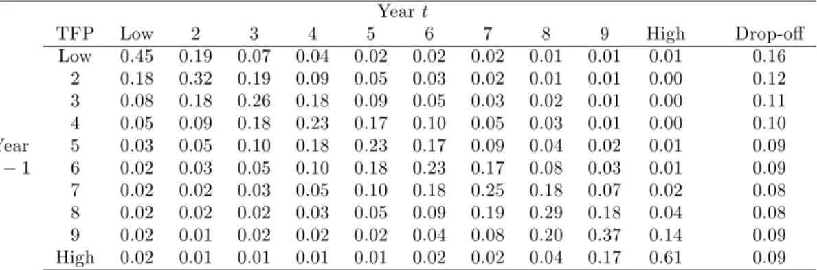
In this section, we present additional information on TFP and the relationship between TFP and …rm characteristics. Table A1 presents the transition probability matrix for the …rms in our sample sorted into decile TFP portfolios. The probabilities of staying in the lowest or the highest TFP portfolios are about 50%. The higher probabilities along the diagonal shows that there is some persistence in productivity.
Table A1 also reports the probability that a …rm in a given portfolio will disappear from our sample in the next year. The drop-o¤ may be the result of either …rm failure or a missing data item in the following year. The probability of drop-o¤ ranges from 8-9% for the …rms in the higher TFP portfolios to 16% for the …rms in the lowest TFP portfolio. The negative relationship between drop-o¤ rates and TFP shows that low productivity …rms are more likely to disappear from our sample where the di¤erence in the drop-o¤ rates can be interpreted as the higher likelihood of failure for low TFP …rms.
Table A1: Portfolio Transition Probabilities Yeart
TFP Low 2 3 4 5 6 7 8 9 High Drop-o¤
Low 0.45 0.19 0.07 0.04 0.02 0.02 0.02 0.01 0.01 0.01 0.16 2 0.18 0.32 0.19 0.09 0.05 0.03 0.02 0.01 0.01 0.00 0.12 3 0.08 0.18 0.26 0.18 0.09 0.05 0.03 0.02 0.01 0.00 0.11 4 0.05 0.09 0.18 0.23 0.17 0.10 0.05 0.03 0.01 0.00 0.10 Year 5 0.03 0.05 0.10 0.18 0.23 0.17 0.09 0.04 0.02 0.01 0.09 t 1 6 0.02 0.03 0.05 0.10 0.18 0.23 0.17 0.08 0.03 0.01 0.09 7 0.02 0.02 0.03 0.05 0.10 0.18 0.25 0.18 0.07 0.02 0.08 8 0.02 0.02 0.02 0.03 0.05 0.09 0.19 0.29 0.18 0.04 0.08 9 0.02 0.01 0.02 0.02 0.02 0.04 0.08 0.20 0.37 0.14 0.09 High 0.02 0.01 0.01 0.01 0.01 0.02 0.02 0.04 0.17 0.61 0.09
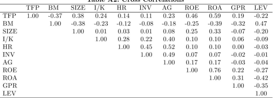
Table A2 presents a cross correlation matrix of …rm level productivity and other …rm level characteristics. We calculate the cross correlations across individual stocks each year and then average them across time. The cross correlation between TFP and B/M is -0.37, TFP and size is 0.38, TFP and investment to capital ratio is 0.24, TFP and the hiring rate is 0.14. The cross correlations between TFP and GPR is 0.19, whereas the cross correlations with ROE and ROA are higher, at 0.46 and 0.59, respectively. The order of magnitude of these correlations are similar to the cross correlations between some of the …rm characteristics. For example, the cross correlation between BM and Size is -0.38, and BM and ROE and ROA are -0.25 and -0.39, respectively. The cross correlations between size and ROE and ROA are 0.25 and 0.33.
Investment to capital ratio is highly correlated with asset growth (0.40), whereas BM is highly correlated with leverage (0.47).
Table A2: Cross Correlations
TFP BM SIZE I/K HR INV AG ROE ROA GPR LEV
TFP 1.00 -0.37 0.38 0.24 0.14 0.11 0.23 0.46 0.59 0.19 -0.22 BM 1.00 -0.38 -0.23 -0.12 -0.08 -0.18 -0.25 -0.39 -0.32 0.47 SIZE 1.00 0.01 0.03 0.01 0.08 0.25 0.33 -0.07 -0.20 I/K 1.00 0.28 0.22 0.40 0.10 0.10 0.06 -0.09 HR 1.00 0.45 0.52 0.10 0.10 0.00 -0.03 INV 1.00 0.49 0.07 0.07 -0.02 -0.01 AG 1.00 0.17 0.17 -0.03 -0.04 ROE 1.00 0.76 0.22 -0.27 ROA 1.00 0.31 -0.42 GPR 1.00 -0.35 LEV 1.00
4
Empirical Robustness Checks
We examine the sensitivity of our production function estimates, our measure of …rm level TFPs, and the resulting relationship between …rm level TFPs, …rm characteristics, and returns to a large number of alternative speci…cation. On the measurement of inputs, we experiment with de…ning the capital stock inclusive of inventories as in Cooley or Prescott (1995), broadening the Olley and Pakes method to include organization capital as another input to the production function14, using a broad de…nition of …xed capital that includes the R&D capital, as well as using di¤erent de‡ators and prices (such as industry de‡ators), carrying out the estimation at the industry level (allowing for di¤erent production function estimates for industries). Our overall results on the relationship between TFP and …rm characteristics and returns are not sensitive to any of these speci…cations. The results are also not sensitive to carrying out the estimation with industry speci…c time dummies at 2, 3, and 4 digit SIC levels. The …ndings are also similar for manufacturing versus non-manufacturing …rms and over di¤erent sample periods.
Following Liu, Whited, and Zhang (2009), we also compute unlevered equity returns and study the relationship between …rm TFPs and future unlevered returns. Both unlevered TFP sorted portfolio returns and Fama-Macbeth regressions with unlevered returns yield results that 1 4We measure organizational capital based on data on …rm’s reported Sales, General, and Administrative
expenses from Compustat (XSGA) as in Eisfeldt and Papanikolaou (forthcoming). We construct it by using the perpetual inventory method where XSGA is de‡ated by the price de‡ator for investment for the matching industry from the NBER-CES Database (PIINV) and assumed to depreciate by 20% per year.
resemble the ones for levered returns. Hence, we con…rm that di¤erences in leverage are not the underlying reason for the spread between the low and high TFP equity returns found previously. Like most variables that predict returns, our results based on realized returns are typically stronger for smaller …rms. Following Fama and French (2008), which puts a special emphasis on micro cap …rms, we replicated our full analysis by excluding micro cap …rms (as de…ned by Fama and French, using the 20th percentile of the NYSE …rm size distribution as the breakpoint) from our sample. As Fama and French (2008) also point out, this leads to eliminating more than half of the sample. In this smaller sample, we …nd that the magnitude of the spreads and coe¢ cients are typically smaller (about half) and less signi…cant (only at 10% level) in tests that use realized returns, though the results are still strong in contractions. But the results of tests that use implied cost of capital remain mostly unchanged.15
December …scal year end requirement and portfolio breakpoints: Tables A3 and A4 reproduce the main results (Table I, Descriptive Statistics, and Table II, Excess Returns) when we drop the December …scal year end requirement, and compute the breakpoints based on the entire cross section of …rms.
1 5
Detailed robustness results were presented in the earlier versions of the paper and are available from the authors upon request.
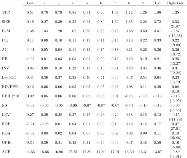
Table A3: Descriptive Statistics for TFP Sorted Portfolios, 1963-2009
Low 2 3 4 5 6 7 8 9 High High-Low
TFP 0.51 0.70 0.79 0.85 0.91 0.96 1.03 1.12 1.26 1.86 1.35 SIZE 0.19 0.27 0.39 0.52 0.68 0.89 1.30 1.65 2.28 3.72 3.53 (21.87) B/M 1.38 1.34 1.20 1.07 0.96 0.86 0.76 0.68 0.59 0.51 -0.87 (-13.38) I/K 0.11 0.09 0.10 0.11 0.13 0.14 0.16 0.18 0.22 0.33 0.22 (19.09) AG -0.01 0.05 0.08 0.11 0.13 0.15 0.18 0.21 0.26 0.36 0.36 (13.72) HR -0.03 0.01 0.03 0.05 0.07 0.09 0.12 0.12 0.19 0.21 0.25 (13.27) INV 0.05 0.08 0.10 0.12 0.13 0.16 0.21 0.23 0.34 0.36 0.31 (12.24) IOC/OC 0.41 0.36 0.37 0.38 0.40 0.41 0.44 0.47 0.54 0.64 0.23 (14.73) RD/PPE 0.12 0.06 0.06 0.05 0.05 0.05 0.06 0.08 0.11 0.20 0.08 (8.18) RER (*10) 0.02 0.05 0.06 0.06 0.02 0.06 0.01 -0.02 -0.05 -0.13 -0.15 (-3.95) NS -0.08 -0.06 -0.06 -0.06 -0.07 -0.07 -0.07 -0.07 -0.10 -0.14 -0.06 (-5.55) LEV 0.27 0.29 0.28 0.27 0.25 0.23 0.20 0.18 0.15 0.12 -0.15 (-11.49) ROE -0.21 -0.05 0.01 0.04 0.07 0.09 0.10 0.12 0.14 0.17 0.37 (27.01) ROA -0.07 0.00 0.02 0.04 0.05 0.06 0.07 0.08 0.09 0.11 0.18 (25.86) GPR 0.34 0.39 0.41 0.43 0.44 0.46 0.46 0.47 0.48 0.50 0.16 (15.00) AGE 14.55 16.66 16.96 17.25 17.39 17.30 17.01 16.50 15.31 13.67 -0.89 (-3.91)
Note: For each variable, averages are …rst taken over all …rms in that portfolio, then over years. On average, there are 187 …rms in each portfolio every year. Average TFP each year is normalized to be 1. SIZE is the market capitalization of …rms in June of year t+ 1. Average size each year is normalized to 1. B/M is the ratio of book equity for the last …scal year-end in year tdivided by market equity in December of year t: I/K is the …xed investment to capital ratio. AG is the change in the natural log of assets, HR is the change in the natural log of number of employees, and INV is the change in the natural log of total inventories, all measured from yeart 1to yeart. Ioc=OCis the ratio of investment
in organization capital to the stock of organization capital in year t, both computed from the de‡ated sales, general and administrative expenses. RD/PPE is the ratio of research and development expenses to gross PPE in yeart. RER is the ratio of buildings +capital leases to PPE in yeart, adjusted for industries. NS is the change in the natural log of the split-adjusted shares outstanding from the …scal year-end int 1tot. LEV is the ratio of long-term debt holdings in year t to the …rm’s total assets calculated as the sum of their long-term debt and the market value of their equity in December of year t. ROE is the net income in yeart divided by book equity for year t. ROA is the net income in year t
in Compustat. N is the average number of …rms in each portfolio in yeart: Table A4: Excess Returns for TFP Sorted Portfolios (%, annualized)
Low 2 3 4 5 6 7 8 9 High High-Low
Contemporaneous Returns, January 1963 - December 2009 re EW -2.96 3.81 7.76 10.32 12.23 13.42 15.29 16.66 18.03 21.84 24.80 (-0.79) (1.20) (2.47) (3.32) (4.08) (4.43) (5.07) (5.49) (5.72) (6.47) (13.79) e EW 25.7 21.8 21.6 21.3 20.6 20.8 20.7 20.8 21.6 23.1 12.3 re V W -7.70 -1.37 1.15 2.80 4.81 5.33 5.53 7.24 5.73 9.29 16.99 (-2.02) (-0.42) (0.40) (1.02) (1.83) (2.09) (2.26) (2.93) (2.35) (3.67) (6.99) e V W 26.10 22.46 19.57 18.84 18.00 17.46 16.82 16.91 16.69 17.35 16.68 Future Returns, July 1964 - June 2011
All states, 564 months
reEW 15.31 13.49 11.98 11.64 10.83 10.48 10.15 9.06 8.63 7.67 -7.65 (4.02) (4.08) (3.87) (3.83) (3.65) (3.49) (3.39) (3.01) (2.78) (2.32) (-4.10) e EW 26.08 22.69 21.22 20.84 20.36 20.56 20.51 20.66 21.31 22.66 12.79 reV W 6.63 7.73 6.86 8.24 7.24 6.36 6.66 4.87 5.68 5.33 -1.29 (1.85) (2.40) (2.44) (2.94) (2.67) (2.47) (2.65) (2.01) (2.29) (2.08) (-0.59) e V W 24.62 22.10 19.26 19.17 18.56 17.65 17.21 16.62 17.01 17.55 15.14 Expansions, 468 months re EW 10.21 9.04 7.78 7.73 7.00 6.76 6.60 5.46 5.12 4.75 -5.46 (2.48) (2.53) (2.33) (2.35) (2.18) (2.06) (2.02) (1.66) (1.52) (1.33) (-2.72) e EW 25.67 22.31 20.84 20.57 20.10 20.50 20.38 20.49 21.08 22.27 12.53 re V W 3.50 5.07 5.19 5.57 4.95 4.38 4.59 2.84 4.37 4.18 0.67 (0.90) (1.47) (1.71) (1.83) (1.68) (1.53) (1.69) (1.07) (1.65) (1.53) (0.27) e V W 24.33 21.49 18.98 18.98 18.42 17.89 16.96 16.56 16.57 17.10 15.38 Contractions, 96 months reEW 40.16 35.20 32.45 30.66 29.48 28.61 27.47 26.61 25.78 21.88 -18.28 (4.21) (4.22) (4.15) (4.06) (4.00) (4.01) (3.79) (3.60) (3.34) (2.56) (-3.79) e EW 26.99 23.57 22.14 21.37 20.85 20.18 20.50 20.88 21.82 24.20 13.65 reV W 21.86 20.67 15.00 21.23 18.39 15.98 16.72 14.75 12.08 10.96 -10.89 (2.41) (2.37) (2.07) (3.04) (2.74) (2.78) (2.60) (2.50) (1.80) (1.58) (-2.26) e V W 25.64 24.62 20.54 19.78 18.98 16.24 18.22 16.67 18.98 19.63 13.65 Note: rEWe is equal-weighted monthly excess returns (excess of risk free rate). reV W is value-weighted monthly excess returns, annualized, averages are taken over time(%). eEW and
e
V W are the corresponding standard deviations. Contemporaneous returns are measured
in the year of the portfolio formation, from January of yeartto December of yeart. Future returns are measured in the year following the portfolio formation, from July of yeart+ 1
to June of yeart+ 2 and annualized(%). t statistics are in parentheses. Expansion and contraction periods are designated in June of year t+ 1based on the level of (one sided HP-…ltered) industrial production in May of that year. Returns over the expansions and contractions are measured from July of yeart+ 1to June of yeart+ 2.
5
Model Details
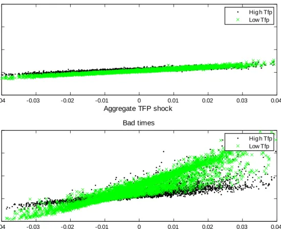
In order to demonstrate the e¤ect of aggregate shocks on low and high TFP …rms over the business cycle, Figure 1 plots the sensitivity of low and high TFP …rms’returns to aggregate TFP shocks conditional on the state of the economy. Good (bad) times are de…ned as times when the last period’s aggregate TFP is more than one standard deviation above (below) its mean. Low (high) TFP …rms are …rms in the lowest (highest) TFP decile based on last year’s ranking. The top panel plots the aggregate shock - realized return (averaged over all low or high TFP …rms every period) relationship in good times, the bottom panel plots the same in bad times. There is a positive relationship between aggregate shocks and realized returns for all …rms and economic environments. However, the relationship is quite ‡at for all …rms in good times, whereas the sensitivity of all …rms, but especially the low TFP …rms, is much higher in bad times. These are the times when low TFP …rms are the riskiest. Bad aggregate shocks lead to very negative returns, whereas good shocks drive the high returns of low TFP …rms in bad times.
6
Numerical Solution
To solve the model numerically, we solve the Euler equation (Equation??) using perturbation methods. We implement …fth-order approximation to the Euler equation and policy functions using Dynare++ software, which is a standalone C++ version of Dynare specialized in com-puting k-order approximations of dynamic stochastic general equilibrium models.16 The main advantage of using perturbation methods/Dynare++, over other numerical techniques, such as value function iterations, parameterized expectations or projection methods, is that it is much faster. The solution of the model on a standard PC takes less than a minute.
We run 500 simulations of 4000 …rms where each simulation runs for 50 periods (roughly matching the length of our empirical sample). We follow Den Haan and De Wind (2009), who advocate running short sample simulations to avoid numerical problems.17 In order to generate the initial conditions (for the cross section of …rms) for the …rst panel, we solve the model using
1 6See www.dynare.org for more information on Dynare and Dynare++.
1 7It is well known that higher-order perturbation solutions might have explosive behavior. Den Haan and
De Wind (2009) suggest using short samples and rejection sampling to deal with these cases. We follow their suggestions, and con…rm that the fraction of discarded samples is very low.
-0.04-1 -0.03 -0.02 -0.01 0 0.01 0.02 0.03 0.04 0 1 2 3 Good times Aggregate TFP shock % R eal iz e d ret ur n Hig h Tfp Low Tfp -0.04-1 -0.03 -0.02 -0.01 0 0.01 0.02 0.03 0.04 0 1 2 3 Bad times Aggregate TFP shock % R eal iz e d ret ur n Hig h Tfp Low Tfp
Figure 1: Sensitivity of …rm returns to aggregate shocks. Top …gure plots the realized returns as a function of aggregate productivity for low TFP and high TFP …rms in good times. Bottom …gure plots the realized returns in bad times.
…rst-order approximation, simulate the model for a long period of time (20000 periods) for a cross section of …rms (4000 …rms), and use the ending distribution of TFP and capital holdings as the starting point for the simulations of the …fth-order solution. For consecutive short sample simulations, the ending distribution of one simulation serves as the initial conditions of the next panel. Once the simulations are completed, we calculate statistics of each sample and compute the con…dence intervals around the statistics.
References
[1] Brynjolfsson, E. and L. Hitt. 2003. Computing Productivity: Firm-Level Evidence.Review of Economics and Statistics 85:793-808.
[2] Cooley, T. F., and E. C. Prescott. 1995. Economic Growth and Business Cycles. In T. F. Cooley (ed.),Frontiers of Business Cycle Research, Princeton University Press.
[3] Den Haan, W. J. and J. De Wind. 2009. How Well-Behaved are Higher-Order Perturbation Solutions? Working Paper, University of Amsterdam.
[4] Eisfeldt, L. A. and D. Papanikolaou. Forthcoming. Organization Capital and the Cross-Section of Expected Returns.Journal of Finance.
[5] Fama, E. F. and K. R. French. 2008. Dissecting anomalies.Journal of Finance 63:1653-78. [6] Fama, E. F. and J. D. MacBeth. 1973. Risk, return, and equilibrium: Empirical tests.
Journal of Political Economy 81:607-36.
[7] Fernández-Villaverde, J. and J. F. Rubio-Ramírez. 2007. On the solution of the growth model with investment-speci…c technological change. Applied Economics Letters 14:533-49.
[8] Foster, L., J. Haltiwagner, and C. Syverson. 2008. Reallocation, Firm Turnover and E¢ -ciency: Selection on Productivity or Pro…tability.American Economic Review 98:394-425. [9] Greenwood, J., Z. Hercowitz, and P. Krusell. 1997. Long-Run Implications of
Investment-Speci…c Technological Change. American Economic Review 87:342-62.
[10] Greenwood, J., Z. Hercowitz, and P. Krusell. 2000. The Role of Investment-Speci…c Tech-nological Change in the Business Cycle.European Economic Review 44:91-115.
[11] Hall, B. H. 1990. The Manufacturing Sector Master File: 1959-1987. NBER Working paper 3366.
[12] Hulten, C. R. 1990. The Measurement of Capital. In Ernst R. Berndt and Jack E. Triplett (eds.),Fifty Years of Economic Measurement: The Jubilee of the Conference on Research
in Income and Wealth. NBER Studies in Income and Wealth 54:119-52. University of
Chicago Press.
[13] Levinsohn, J. and A. Petrin. 2003. Estimating Production Functions Using Inputs to Con-trol for Unobservables.Review of Economic Studies 70:317–41.
[14] Liu, L. X., T. M. Whited and L. Zhang. 2009. Investment-Based Expected Stock Returns. Journal of Political Economy 117:1105–39.
[15] Novy-Marx, R. Forthcoming. The Other Side of Value: The Gross Pro…tability Premium. Journal of Financial Economics.
[16] Olley, S. and A. Pakes. 1996. The Dynamics Of Productivity In The Telecommunications Equipment Industry.Econometrica 64:1263-97.