Water networks security: A two-stage mixed-integer stochastic program for sensor placement under uncertainty

(1)

Water networks security: A two-stage mixed-integer stochastic

program for sensor placement under uncertainty

夽

Vicente Rico-Ramirez

a,∗

, Sergio Frausto-Hernandez

a

,

Urmila M. Diwekar

b

, Salvador Hernandez-Castro

c

a_{Instituto Tecnologico de Celaya, Departamento de Ingenieria Quimica, Ave, Tecnologico y Garcia Cubas S/N, Celaya, Gto., C.P. 38010, Mexico} b_{Vishwamitra Research Institute, 34 N. Cass Avenue, Westmont, IL 60559, USA}

c_{Universidad de Guanajuato, Facultad de Quimica, Col. Noria Alta S/N, Guanajuato, Gto., C.P. 36050, Mexico} Received 15 November 2005; received in revised form 7 August 2006; accepted 17 August 2006

Available online 27 September 2006

Abstract

This work describes a stochastic approach for the optimal placement of sensors in municipal water networks to detect maliciously injected con-taminants. The model minimizes the expected fraction of the population at risk and the cost of the sensors. Our work explicitly includes uncertainties in the attack risk and population density, so that the resulting problem involves optimization under uncertainty. In our formulation, we include the location of a number of sensors as first stage decision variables of a two-stage mixed-integer stochastic linear problem; the second stage evaluates the population at risk for the scenario obtained in the first stage and that information is then used to modify the first stage decisions for the next iteration. Since the model is integer in the first stage, a generalized framework based on the stochastic decomposition algorithm allows us to solve the problem in a reasonable computational time. The paper describes the mixed-integer stochastic model and the algorithmic framework, and com-pares the deterministic and stochastic optimal solutions. The network used as our case study has been derived through the water network simulator EPANET 1.0; four acyclic water flow patterns are considered. Results show a significant effect of uncertainty in sensor placement and total cost. © 2006 Elsevier Ltd. All rights reserved.

Keywords: Mixed-integer stochastic programming; Stochastic decomposition; Water networks security

1. Introduction

Stochastic programming has become a common tool for deci-sion making on process design, production planning, location, scheduling and finance. Hence, literature in the last decade reports many papers that have addressed the issue of solving opti-mization problems under uncertainty;Sahinidis (2004)provided an excellent review on the various applications and opportunities of this area.

Several modeling approaches based on a variety of philoso-phies have been proposed. Among the applications on process systems engineering, most of the methods can be classified into one of the following two categories: (1) integration methods and (2) sampling methods.Acevedo and Pistikopoulos (1998) com-pared the Gaussian Quadrature formula (integration method)

夽 _{A preliminary version of this paper was presented at the ESCAPE-15}

Con-ference.

∗_{Corresponding author. Tel.: +52 461 6117575; fax: +52 461 6117744.}

E-mail address:[email protected](V. Rico-Ramirez).

with Monte Carlo sampling for sample average approximation.

Wei and Realff (2004) also presented a review on this issue and developed two sample average approximation methods (optimality gap and confidence level) for solving convex stochastic MINLPs. Similarly, Novak Pintaric and Kravanja (2004) presented a sequential two-stage strategy for the stochastic synthesis of chemical processes, in which flexibility and static operability are simultaneously taken into account.

In addition, a number of contributions have recently been reported to approach the solution of deterministic and stochastic problems of optimal sensor placement. For instance,

Bagajewicz, Fuxman, and Uribe (2004) developed a mixed-integer linear programming formulation for the design of sensor networks for simultaneous process monitoring and fault detection/resolution.

This paper describes a stochastic approach for the optimal placement of sensors in municipal water networks to detect maliciously injected contaminants. This approach represents yet another application of stochastic programming, and it is relevant in the context of homeland security efforts.

(2)

1.1. Optimal placement of sensors in municipal water networks: a stochastic approach

Recently,Berry, Fletcher, Hart, and Philips (2003)presented a mixed-integer linear programming (MIP) formulation for opti-mal placement of sensors in municipal water networks to quickly detect accidental or malicious contamination of the system. Such a formulation seeks to minimize the expected fraction of the population at risk. An attack is modeled as the release of a large volume of harmful contaminant at a single point in the network with a single injection. In general, it is difficult to know a priori where an attack will occur, so, a compromise solution across a set of weighted attack scenarios is generated. For each flow pat-tern, each node is weighted by the number of people (population density) potentially consuming water at that point. The result-ing MIP formulation assumes constant probabilities for attack risks and population densities, making the problem a determin-istic MIP. Nevertheless, the results of the analysis show that the optimal configuration is a strong function of the fixed number of sensors used in the formulation. Also, the model does not include the cost and type of the sensors, which could be major factors in the solution achieved. Further, although uncertainties in the demand and variability in the population density can impact the solution, they are not formally considered.

Our work proposes extensions to such a model to explicitly include uncertainties in attack risks and population density. This changes the problem to an optimization under uncertainty prob-lem (stochastic programming probprob-lem). In our formulation, we include the number and location of the sensors as first stage deci-sion variables of a two-stage mixed-integer stochastic problem, where the costs of sensors are included in the objective function. Hence, the stochastic mixed-integer linear program is solved by applying the stochastic decomposition (SD) algorithm ofHigle and Sen (1991).

1.2. Two-stage stochastic programming and the SD algorithm

The basic SD algorithm (Higle & Sen, 1991) was developed to solve stochastic linear problems with recourse (SLPwR). The main class ofSLPwRproblems involves two stages. In the first stage, the choice of the (first stage) decision variablesxis made. In the second stage, following the observation of the values of the uncertain parameters,ω, and the evaluation of the objective function, a corrective action (represented by the second stage decisions),y, is suggested. The standard mathematical form of a

SLPwRproblem is given by Eqs.(1)and(2). Eq.(1)is referred as the first stage problem:

MincTx+Q(x) Subject to :

Ax=b

x≥0 (1)

whereAis a coefficient matrix,cthe coefficient vector andQ(x) is the recourse function defined byQ(x) =E[Q(x,ω)].Eis the

expectation operator and Q(x,ω) is obtained from the second stage problem, Eq.(2):

Q(x, ω)=MinqTy Subject to :

W(ω)y=h(ω)−T(ω)x

y≥0 (2)

In Eq.(2),qis a coefficient vector andW,handTare coeffi-cient matrices which in principle might depend on the random variablesω. The theory and steps of the basic SD algorithm can be found inHigle and Sen (1996)andPonce-Ortega, Rico-Ram´ırez, Hernandez-Castro, and Diwekar (2004); a step-by-step illustrative example can also be reviewed inRico-Ram´ırez (2002). Seeking completeness, a summary is provided here.

• Step 0: Set the iteration counterν= 0,V0={∅}andθν=−∞.

The initial values of the first decision variables, x1, are assumed as given.

• Step 1: Setν=ν+ 1 and sample to generate an observationων independent of any previous observation.

• Step 2: Determine the coefficients of a piecewise linear approximation to the recourse function,Q(x):

(a) Solve the dual program of the second stage problem MaxπT(h_v−T_vxv)

subject to : πTW ≤q

π≥0

to find the values of the vector of the second stage dual variables (Lagrange multipliers of primal restrictions)π,

πν

ν, and makeVν=Vν−1∪πν_ν.

(b) Get the coefficients of the optimality cut:

αν_v= 1_v v k=1 (πv_k)Th_k βν v= 1_v v k=1 (πv_k)TT_k

whereπ_kνis the solution to the problem (for allk|k=ν): MaxπT(h_k−T_kxv)

subject to : π∈V_v

Observe that the solution vector to this problem can only be one of the vectors already included in the set of solu-tions,V_ν(the solution set is restricted to decrease effort). (c) Update the coefficients of previous cuts:

αv_k= v−_v 1αv−1

k , k=1, . . . , v−1

βv_k= v−_v 1βv−1

k , k=1, . . . , v−1.

• Step 3: Solve the first stage problem after the addition of the optimality cut: MincTx+θν subject to : Ax=b θv₊_βv kx≥αvk, k=1, . . . , v x≥0, θν∈ to obtainxν+1. Go to Step 1.

(3)

• There are several stopping criteria for the algorithm; in the most simple case, the algorithm stops if:

(a) change in the objective function is small;

(b) no new dual vectors are added to the set of dual solutions,

V.

One can observe that the first and the second stages of the problem are both linear programs. Also, as can be reviewed in the text by Birge and Louveaux (1997), if the first stage becomes a mixed-integer linear program (x∈{0,1}as opposed to x≥0), the basic steps of the algorithm hold. However, if the second stage becomes a mixed-integer program (y∈{0,1} as opposed to y≥0), then the derivation of the optimality cut (Step 2) involves a branch and bound strategy where, besides seeking feasibility and optimality, enforcing integral-ity of the solution greatly complicates the algorithm. Fortu-nately, the resulting stochastic program of this work is first stage integer.

2. Water networks security model: MIP formulation versusSMILPwRformulation

This section describes the MIP approach to represent the water network security problem (Berry et al., 2003) and the reformulation of such model as a stochastic mixed-integer linear programming problem with recourse (SMILPwR). The com-putational implementation of the solution algorithm is also provided.

2.1. MIP formulation ofBerry et al. (2003)

The municipal water network is represented as a directed graphG= (V,E), whereEis the set of edges or pipes (E=e1,. . ., em) andVis a set of vertices or nodes (V =v1, . . . , vn) where the

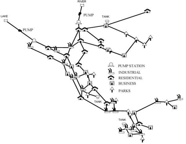
pipes meet. Vertices represent sources (reservoir, tanks) where water is introduced or sinks (demand points) where water is consumed.Fig. 1shows a typical municipal water network con-figuration. Each pipe connects two nodes and is usually denoted as (vi, vj). The analysis is performed under a number of water flow patterns, where the direction of the flow in each pipe is known. The parametersfijpdescribe the pattern;fijpis equal to

1 if there is a positive flow along the directed pipee= (v_i, v_j) during flow patternp, and it is equal to 0 otherwise. The proba-bility of attack for nodev_iduring flow patternpis represented asηip; such that the summation overiof all of the values ofηipis

equal to 1.δipis the population density at nodeviwhile flowpis

active; understanding the value of the population density as the number of individuals consuming water at each particular node. The decision variables,xij, define the sensor placement, and the

derived variables,yipj, define the propagation of an injected

con-taminant. A sensor on pipe (v_i, v_j),xij, detects contaminants

moving on either direction.yipjis equal to 1 if nodev_jis

contam-inated by an attack at nodeviduring patternp, and 0 otherwise. As mentioned before, an attack is the single injection of a large volume of harmful contaminant at a single point, but then all points downstream can be contaminated. Propagation fromv_k tov_j occurs ifv_k is contaminated, there is positive flow from

(4)

Fig. 2. Modeling the propagation of an injected contaminant. (a) Propagation from nodekto nodejoccurs (positive flow). (b) Propagation from nodekto nodejdoes not occur. (c) Sensor prevents propagation from nodekto nodej.

vktov_jand there is no sensor in between.Fig. 2illustrates the model of the contaminant propagation. Finally,Xmaxis the

max-imum number of sensors. The MIP formulation of Berry et al. is given by Eq.(3): Min n i=1 P p=1 n j=1 ηipyipjδjp s.t. yipi=1 ∀i=1, . . . , n, p=1. . . P xij =xji ∀i=1, . . . , n−1, i < j yipj ≥yipk−xkj ∀(k, j)∈E, s.t. f_kjp=1

(i,j)j∈E, i<jxij−Xmax≤0

xij∈ {0,1} ∀(i, j)∈E

(3)

The first constraint of the model ensures contamination of a node when it is directly attacked. The second constraint implies that a sensor on a pipe will detect the contaminant despite the flow direction. The third one is the contaminant propagation constraint. Finally, the last constraint enforces the total num-ber of sensors to be less or equal to the maximum numnum-ber

Xmax. In Eq. (3), ηip and δip are fixed given parameters on

a particular scenario; therefore, the model is a deterministic MIP.

2.2. Reformulation as a SMILPwR

Although the fundamentals of our model are the same as those proposed by Berry et al. (2003), our main contri-bution is the reformulation of the problem as a first stage integer, two-stage stochastic mixed-integer linear problem. That is significant for two reasons: (i) first, the uncertain-ties are formally incorporated into the model and (ii) the basic stochastic decomposition algorithm (Higle & Sen, 1991) can be used to provide the optimal solution to the problem.

Our work explicitly includes uncertainties in risk of attack,

ηip, and population density, δip. An assumed probability

distribution function is assigned to each of those parameters. That consideration makes the problem a stochastic program. Notice that the symbolωwas used in Section1to represent the uncertain parameters. Hence, in ourSMILPwRformulation, the vectorωconsists of all of the values of both parameters, risk of attack,η, and population density,δ, and such values change for each nodeiand flow patternp. Uncertainty in population density is assumed because the model consider a 24 h cycle; although during that period the total population remains basically the same, the transit of people among different nodes makes it diffi-cult to predict the exact number of individuals at each particular node.

Also, we proposed the separation of the model constraints into two stages, following the concept of recourse. The first stage includes the decisions about the placement of the sensor through the binary variablesxij. Also, the costs of the sensors (and sensor

placement),Cij, are included in the first stage objective function.

Hence, by including such costs, the optimal solution may not use the total number of sensors and, therefore, the number of sensors in the configuration also becomes an optimization variable.

The derived variables (which represent the propagation of contaminants), yipj, are then considered as the second stage

decisions. The recourse function (expected value of the second stage objective function) is almost identical to the objective function of the original MIP model. It includes the calculation of the population at risk under an attack. However, a factorS

has been added to the calculation.Sis a cost associated per each member of the population which suffers from the attack. So, the first stage tries to minimize the cost of the sensors as well as the expected value (Eω) of the cost associated to the population suffering the attack (computed through the objective of stage two); notice then that both terms are calculated in a monetary basis. Nevertheless, Cij andS might simply be interpreted as

(5)

weighting (or scaling) factors from the numerical point of view.

In summary, the two-stage approach works as follows: (i) the first stage decides about the number and the loca-tion of the sensors; (ii) given the first stage decisions, for some sampled values of the uncertain parameters, the sec-ond stage evaluates the population at risk for that scenario; (iii) the second stage objective function calculation is then used (through an optimality cut) to modify the first stage decisions for the next iteration; that is precisely the idea of recourse.

Eqs.(4)and(5)show the constraints of the two stages. The constraints of the first stage impose a number of sensors (less or equal to the maximum) to be placed in the network. The con-straints in the second stage propagate contamination if there is no sensor that prevents it and evaluate the population at risk under an attack. Notice that the first stage is an integer programming problem.

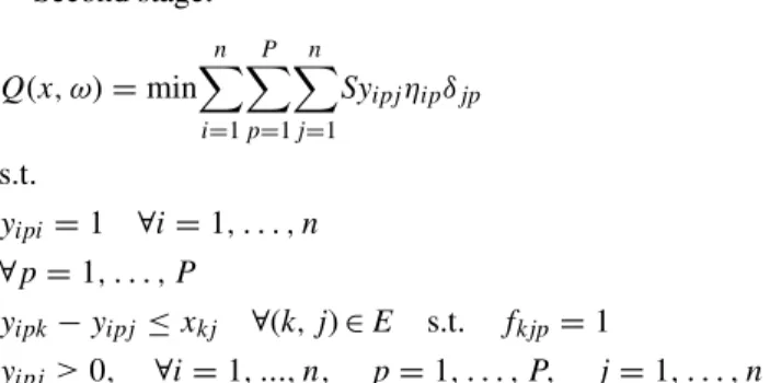
First stage (integer): Min n i=1 n j=1 Cijxij+Eω[Q(x, ω)] s.t. xij−xji=0 ∀i=1, ..., n−1, i < j (i,j)j∈E,i<j xij−Xmax≤0 xij∈ {0,1} ∀i, j∈E (4) Second stage: Q(x, ω)=min n i=1 P p=1 n j=1 Syipjηipδjp s.t. yipi=1 ∀i=1, . . . , n ∀p=1, . . . , P yipk−yipj≤xkj ∀(k, j)∈E s.t. f_kjp=1 yipj ≥0, ∀i=1, ..., n, p=1, . . . , P, j=1, . . . , n (5)

2.3. The solution approach for the SMILPwR model

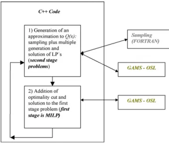
Because the problem is integer in the first stage, the solution can be achieved with the same basic steps of the SD algorithm developed for linear problems; the only difference is that, instead of a linear problem, now an integer linear programming problem has to be solved in order to find the first stage decisions in each of the iterations.Fig. 3shows a flowsheet of the solution steps. Our computational implementation of the algorithm involves a framework that integrates the Hammersley sequence sampling technique (Kalagnanam & Diwekar, 1997) coded in FORTRAN, the GAMS modeling environment (Brooke, Kendrick, Meeraus, & Raman, 1998), and a C++ manager program. The manager program generates the appropriate MILP and LP problems for each of the SD iterations, transfers the control of execution and verifies the convergence of the algorithm.Fig. 4represents the computational implementation of the algorithm.

(6)

Fig. 4. Computational implementation. 3. Illustrative example and results

This section presents the solution of example network number 2 of EPANET 1.0 (Rossman, 1999). The water network is shown inFig. 5a. It has 36 nodes and 40 pipes with 1 pump station and 1 storage tank. The EPANET example assumes as given 4 time periods (4 water flow patterns, i.e., different directions of flow) of 6 h in a 24 h total period.Fig. 5b shows one of the flow patterns used. Also, the nodes are distributed in 4 zones: pump station, residential neighborhood, business district and industrial district; see Table 1 for the node distribution. The maximum number of sensors is seven. The definition of the four zones, the node distribution and the value of the maximum number of sensors are the same as those provided by the EPANET case-study and used byBerry et al. (2003)while solving the deterministic case. For testing purposes, we assign

Table 1

Distribution of nodes of the network

Zone Nodes Total

Pump station 1 1

Industrial district 3, 10, 11, 12, 16, 17, 18, 20, 21, 22, 26, 30 12 Residential neighborhood 2, 4, 5, 6, 8, 9, 19, 23, 27, 28, 31, 32 12 Business district 7, 13, 14, 15, 24, 25, 29, 33, 34, 35, 36 11

normal and triangular distributions to the population density. For the normal distribution, we assume a mean equal to 500 and a standard deviation of 63 (about 95% probability of having values between 375 and 625). For the triangular distribution, we consider a minimum of 375, a maximum of 625 and a mode of 500. The same probability distribution was assumed for each node and an independent sampling was performed for each of them (that is, 36 values are sampled). After sampling, the values are normalized so that the total population is always 18,000. Hence, the normalized valuesδ_ipfor the population density can be calculated from the sampled valuesδipby using Eq.(6):

δip =18,000δ₃₆ip i δip.

(6) A normal distribution is assumed for the probability of attack. For this case, however, all of the nodes in the same zone are assumed to have the same probability of being attacked (only four values of probability of attack are sampled). Four possible scenarios are considered.Table 2shows the probability data for each of the four scenarios. Values inTable 2do not necessarily correspond to realistic expectations of the probability of attack; they represent instances of situations in which the probability of attacking a particular zone is much higher than those of the other zones. With such selections, we intend to find how significant is the location of the attack in the optimal sensor configuration. The sampled values of the probability of attack are also

(7)

Table 2

Mean values of the probability of attack used for each zone and scenario Scenario Probability of attack (%)

Pump station Industrial Residential Business

1 65 12 12 11

2 1 76 12 11

3 1 12 76 11

4 1 12 12 75

ized so that their sum is 1. Therefore, information ofTable 2

implies for instance that, for the scenario 3, the probability of attack of all of the nodes of the residential neighborhood is the same for each of them, and their sum is approximately 0.76 (0.76 is the mean of the normal distribution for such a zone). Standard deviations for the probability of attack are chosen so that there is a 95% probability that the sampled values are found between±25% of their mean value (25% of the mean value is approximately equal to 2S.D.). In addition, two costs for sensors are used: low (15,000,000) and high (45,000,000). Finally, the cost associated (S) per each affected individual is 30,000. Such values are assumed as constant and were selected in such a way that both of the terms of the objective function of Eq.(4)have the same order of magnitude. That tried to avoid

trivial solutions in which the optimal configurations suggest either no installation of sensors or installation of one sensor at each node. As mentioned before, one can also interpret those constant values as weights (or scaling factors) in the objective function. The number of samples and iterations of the SD algorithm was 400 with a computational time of 28 min and 30 s (Intel Pentium processor, 1.73 GHz). The stopping criterion used corresponds to that of the basic SD algorithm; the algorithm stops when the relative change of the objective function from one iteration to the next one is less than a given tolerance (1×10−3 _{in this case).} _{Table 3} _{shows the optimal}

stochastic solutions for the scenario where the residential neighborhood is under risk. The deterministic solution is also presented. The deterministic case was solved by using the mean values of the stochastic parameters; for population density, the mean value is 500. The solutions for the other three scenarios present similar behaviors. Such results are shown in

Tables 4–6.

4. Analysis of results

There are meaningful differences among the cases of high and low sensor costs, and even more significant between the stochastic and deterministic cases; on the contrary, the effect of

Table 3

Results for the residential neighborhood

Population density Sensor cost Variable Stochastic solution Deterministic solution Triangular Low Sensors allocated X6–7,X12–13,X14–15,X28–30,X31–32,X32–33,X35–36 X6–7,X12–13,X27–28,X31–32

Population affected (%) 13.64 30.71

Total cost 1.7866887E+8 2.2585000E+8

High Sensors allocated X6–7,X12–13,X27–28,X28–30 X6–7,X28–30

Total cost 3.2145500E+8 3.2010000E+8

Normal Low Sensors allocated X5–6,X6–7,X7–8,X11–12,X19–18,X31–32,X35–36 X6–7,X12–13,X27–28,X31–32

Total cost 1.7781497E+8 2.2585000E+8

High Sensors allocated X6–7,X28–30,X31–32 X6–7,X28–30

Total cost 3.2507400E+8 3.2010000E+8

Table 4

Results for the industrial district

Population density Sensor cost Variable Stochastic solution Deterministic solution Triangular Low Sensors allocated X4–5,X5–6,X11–12,X12–13,X26–27,X31–32,X33–34 X5–6,X12–13,X26–27,X30–31

Total cost 1.8783120E+8 2.2485000E+8

High Sensors allocated X5–6,X12–13,X26–27,X28–30 X12–13,X26–27

Total cost 3.2886790E+8 3.2825000E+8

Normal Low Sensors allocated X5–6,X11–12,X13–14,X15–26,X30–31,X31–32,X35–36 X5–6,X12–13,X26–27,X30–31

Total cost 1.9124361E+8 2.2485000E+8

High Sensors allocated X12–13,X26–27 X12–13,X26–27

(8)

Table 5

Results for the business district

Population density Sensor cost Variable Stochastic solution Deterministic solution

Triangular Low Sensors allocated X6–7,X7–10,X13–20,X14–15,X14–21,X15–26,X26–27 X7–8,X7–10,X13–20,X14–15,X14–21,X26–27

Total cost 2.1854458E+8 2.3097294E+8

High Sensors allocated X11–12,X15–26,X27–28,X30–31,X32–33 X7–10,X14–21,X15–26

Total cost 3.4571300E+8 3.4070487E+8

Normal Low Sensors allocated X7–10,X11–12,X13–20,X14–15,X14–21,X27–28,X28–30 X7–8,X7–10,X13–20,X14–15,X14–21,X26–27

Total cost 2.1456336E+8 2.3097294E+8

High Sensors allocated X11–12,X14–21,X15–26 X7–10,X14–21,X15–26

Total cost 3.4403738E+8 3.4070487E+8

Table 6

Results for the pump station

Population density Sensor cost Variable Stochastic solution Deterministic solution Triangular Low Sensors allocated X1–2,X10–11,X12–13,X19–18,X30–31,X32–33 X1–2,X6–7,X12–13,X27–28

Total cost 9.1588195E+7 1.7505000E+8

High Sensors allocated X1–2,X7–10,X15–26,X23–24,X31–32 X1–2,X12–13

Total cost 2.4416009E+8 2.5455000E+8

Normal Low Sensors allocated X1–2,X11–12,X15–26,X23–24,X28–30,X32–35 X1–2,X6–7,X12–13,X27–28

Total cost 8.9214319E+7 1.7505000E+8

High Sensors allocated X1–2,X7–8,X11–12,X26–27,X30–31 X1–2,X12–13

Total cost 2.464705E+8 2.5455000E+8

the distribution used for the population density seems not to be important:

(a) The number of sensors used and the optimal sensor con-figuration change with respect to the cost of the sensors. In general, one could expect that the fraction of the pop-ulation at risk decreases as one increases the number of sensors; hence, when using cheap sensors, the number of sensors placed tends to the maximum. However, because of the compromise between the cost of the sensors and the associated cost per each affected person, the optimal con-figuration does not always include the maximum number allowed. That is particularly true for the case of expensive sensors.

(b) The probability of attack has a much bigger impact than population density.

(c) Stochastic results are significantly different from deter-ministic results when using cheap sensors. In most cases, the percentage of population under risk is smaller in the stochastic case. There are only two cases where the opposite situation happens (business and industrial districts with normal population density distribution and high sensor cost). We believe, however, that determining which one of two approaches provides lower values for the objective

function is not the main result, but the difference between such values. Notice that a deterministic solution can both overestimate or underestimate the solution because of lack of information; our opinion is then that the stochastic solution, which uses multiples scenarios to generate the solution, will in general provide a better estimate of expected value of the objective function. Table 7 shows the values of the stochastic solution (VSS) for each of the cases considered. VSS represents the difference between the objective functions of the stochastic and deterministic optimal solutions. We can observe values as high as 96% as a consequence of the major impact of uncertainty in the solution.

Table 7

Value of the stochastic solution for each zone and scenario Population

density

Sensor cost

Value of stochastic solution (%)

Pump station Industrial Residential Business

Triangular Low 91.12 19.70 26.40 5.68

High 4.25 0.18 0.42 1.44

Normal Low 96.21 17.57 27.01 7.64

(9)

(d) The effect of uncertainty on the sensor configuration decreases when expensive sensors are used: sensors tend to be placed in nodes with the highest population density. In a realistic situation, one would know the cost of the sensors (and the maximum number of them) and would expect to have a good idea of the distribution function for the population density; hence, the probability of attack would be the most significant of the parameters of the proposed formulation, but it would also be the most difficult to model. The optimal sensor placement suggested by our approach would have to be the one determined through the best possible approximation for the probability of attack that the available information would allow us to obtain.

On the other hand, since the first stage of the problem is a MIP model and this stage has to be solved for every sample (iter-ation), an increment in the number of nodes (and, therefore, in the number of edges) largely increases the combinatorial com-plexity of a problem. This is significant, since literature reports realistic networks with as many as 400 nodes. Hence, the pro-posed formulation would still be applicable, but the basic SD algorithm would have to be modified; problems of such size require a more efficient stopping criterion. The use of incum-bent solutions (Higle & Sen, 1996) can then be thought as a feasible alternative.

5. Conclusions

This paper proposes a two-stage mixed-integer stochastic lin-ear programming approach for the optimal placement of sensors in a municipal water network. Three main results can be summa-rized: (i) first, this approach not only allows the incorporation of uncertainties to the problem but also provides an efficient solution strategy through the SD algorithm, (ii) the results of the illustrative example (VSS, optimal placement and effect to population) reveal the significant effect of the uncertainties in the optimal solution of the problem and (iii) with respect to the parameters under investigation, probabilities of attack and sen-sor cost seem to have a more important effect than that of the population density; that applies for both the stochastic and the deterministic case.

Acknowledgement

Vicente Rico-Ramirez would like to thank the financial support received trough the collaborative research grant NSF-CONACYT 35974-A (Mexico).

References

Acevedo, J., & Pistikopoulos, E. N. (1998). Stochastic optimization based algo-rithms for process synthesis under uncertainty.Computers and Chemical Engineering,22, 647–671.

Bagajewicz, M., Fuxman, A., & Uribe, A. (2004). Instrumentation network design and upgrade for process monitoring and fault detection.AIChE Jour-nal,50, 1870–1880.

Berry, J., Fletcher, L., Hart, W., & Philips, C. (2003). Optimal sensor place-ment in municipal water networks. InProceedings of the world water and environmental resources conference.

Birge, J. R., & Louveaux, F. (1997).Introduction to stochastic programming. New York, NY, USA: Springer-Verlag.

Brooke, A., Kendrick, D., Meeraus, A., & Raman, R. (1998).GAMS-A user guide. Washington, DC, USA: GAMS Development Corporation. Higle, J. L., & Sen, S. (1991). Stochastic decomposition: An algorithm for

two-stage linear programs with recourse.Mathematics of Operations Research,

16, 650–669.

Higle, J. L., & Sen, S. (1996).Stochastic decomposition. New York, NY, USA: Kluwer Academic Publisher.

Kalagnanam, J., & Diwekar, U. M. (1997). An efficient sampling technique for off-line quality control.Technometrics,39(3), 308.

Novak Pintaric, Z., & Kravanja, Z. (2004). A strategy for MINLP synthesis of flexible and operable processes.Computers and Chemical Engineering,28, 1105–1119.

Ponce-Ortega, J. M., Rico-Ram´ırez, V., Hernandez-Castro, S., & Diwekar, U. M. (2004). Improving convergence of the stochastic decomposition algo-rithm by using an efficient sampling technique.Computers and Chemical Engineering,28, 767–773.

Rico-Ram´ırez, V. (2002). Two-stage stochastic linear programming: A tutorial.

SIAG/OPT Views and News,13(1), 8–14.

Rossman, L. A. (1999). The EPANET programmer’s toolkit for analysis of water distribution systems. InProceedings of the annual water resources planning and management conference.

Sahinidis, N. V. (2004). Optimization under uncertainty: State-of-the-art and opportunities. Computers and Chemical Engineering, 28, 971– 983.

Wei, J., & Realff, M. (2004). Sample average approximation methods for stochastic MINLPs. Computers and Chemical Engineering, 28, 333.