FAST AND ACCURATE THREE-DIMENSIONAL RECONSTRUCTION FROM CONE-BEAM PROJECTION DATA USING ALGEBRAIC METHODS DISSERTATION

FAST AND ACCURATE THREE-DIMENSIONAL RECONSTRUCTION FROM CONE-BEAM PROJECTION DATA USING ALGEBRAIC METHODS

DISSERTATION

Presented in Partial Fulfillment of the Requirements for the Degree Doctor of Philosophy in the Graduate

School of The Ohio State University By

Klaus Mueller, Dipl. Ing. (FH), M.S., M.S. * * * * *

The Ohio State University 1998

Dissertation Committee: Dr. Roni Yagel, Adviser Dr. Roger Crawfis Dr. Richard Parent

Approved by

Adviser

© Klaus Mueller, 1998 All Rights reserved.

ABSTRACT

Cone-beam computed tomography (CT) is an emerging imaging technology, as it provides all projections needed for three-dimensional (3D) reconstruction in a single spin of the X-ray source-detector pair. This facilitates fast, low-dose data acquisition as required for imaging fast moving objects, such as the heart, and intra-operative CT applications. Current cone-beam reconstruction algorithms mainly employ the Filtered-Backprojection (FBP) approach. In this dissertation, a different class of reconstruction algorithms is studied: the algebraic reconstruction methods. Algebraic reconstruction starts from an initial guess for the reconstructed object and then performs a sequence of iterative grid projections and cor-rection backprojections until the reconstruction has converged. Algebraic methods have many advantages over FBP, such as better noise tolerance and better handling of sparse and non-uniformly distributed projection datasets. So far, the main repellant for using algebraic methods in routine clinical situations was their slow speed. Apart from providing solutions for this pressing problem, we will also apply, for the first time, algebraic methods in the context of general low-contrast cone-beam tomography. This new context poses several challenges, both for reconstruction quality and speed.

To eliminate the strong aliasing effects that occur when standard algebraic methods are applied for cone angles exceeding 20˚, we introduce the new concept of depth-adaptive basis function kernels. Then, a comprehensive study is conducted on how various parame-ters, such as grid initialization, relaxation coefficient, number of iterations, and correction method (ART or SART) influence cone-beam reconstruction quality and speed. Finally, a new algorithm, the Weighted Distance Scheme, is proposed that optimally arranges the order in which the grid projections are performed., which reduces the number of iterations and promotes reconstruction quality. We find that three iterations are sufficient to obtain good reconstruction quality in the general case. A cost function is then developed that relates the computational effort of FBP with that of algebraic methods. In an attempt to match the cost of algebraic methods and FBP, a new accurate and efficient projection algo-rithm is proposed that reaches its goal by caching projection computations for reuse in the subsequent backprojection. Finally, we propose a new hardware-accelerated scheme for algebraic methods that utilizes readily available off-the-shelf graphics hardware and enables a reconstruction to be performed in less than 2 minutes at good quality.

ACKNOWLEDGMENTS

If you spend ten years of your life at one place, like I did at Ohio State, you will get to know a wide variety of people that are affiliated with this institution in one way or the other. Many of these people will be instrumental in the success of your work, and without their help and inspiration you will never reach your goals, or even be able to discover and define them. My path since arriving from Germany with two suitcases in my hands to the present load, filling a medium sized U-Haul truck, was lined with some of the nicest and most resourceful people I have ever met in my life. I was able to build many incredible friend-ships and collaborations, and I fondly look back to my time as a graduate student at Ohio State.

The person who, without a doubt, has inspired and supported me the most is my advisor Roni Yagel, a mentor par excellence. A meeting with him was like a complete mental over-haul: I would walk into his office, deeply worried about some matter, and would leave an hour later, re-vitalized and full of hope, eager to attack the problem, whatever it was. There was never a time where he could not spare a moment - and often, a moment turned into an hour and more. His optimism, enthusiasm, keen sense for opportunity, ingenuity, and friendship have taught me a great deal and have helped me to grow into a person much more mature than I was when I first met him in 1992.

Another person I am deeply indebted to is Ed Herderick of the Biomedical Engineering (BME) Center at Ohio State, whom I have known almost since my beginnings at this uni-versity. He was the one who recommended me for my first assistantship, inspired, super-vised, and guided me through my Master’s thesis at BME, and provided me with support ever since, even after my departure from BME. The road of this dissertation would have been a lot rockier without his permission to maintain my “home” at the Laboratory of Vas-cular Diseases, whose splendid and neatly maintained computational resources and com-fortable premises have made it so much easier to accomplish this research. In this respect, I also thank Dr. Mort Friedman, Acting Chairman of BME, for generously letting me heat the BME CPU’s and spin 3 GB of harddrive real-estate over the past two years. Thanks are especially in order for BME system administrator Vlad Marukhlenko who kept the CPU’s heatable, the harddrives spinable, and the cooling fans quiet.

Enthusiastic thank-you’s go out to a number of people that have provided me with research opportunities and financial backing, and who have trusted in me that I could actually per-form the work that had to be done. First, I must thank Prof. Herman Weed, and also Dr. Richard Campbell, who admitted me to the BME program in a rather un-bureaucratic man-ner, not knowing much about me other than my grades and the fact that I was German. When I arrived in Columbus one cold winter day in 1988, the wind hissing around the

cor-ners of Dreese Laboratories, Prof. Weed and Dr. Campbell quickly integrated me into the program, and made sure I wouldn’t get lost so far away from home.

I am also greatly indebted to Dr. J. Fredrick Cornhill, who became my advisor shortly after my arrival in the US and who would let me do computer-related research even though I, as an electrical engineer, was initially not very versed in these aspects. This early research sparked my interest in computer science, and Dr. Cornhill’s generous funding for the next seven years enabled me to deeply acquaint myself with the subject, a task that ultimately lead to a second Master’s degree in that discipline (and subsequently this Ph.D.). I want to thank Dr. Cornhill for providing me with the opportunity to participate in a number of clin-ical software projects at the Cleveland Clinic Foundation. This involvement in real-life applications of computers in the medical field have surely prepared me well for a career that is geared towards the development of practical systems that benefit human health and well-being.

I would also like to thank Dr. John Wheller, head of the Columbus Children’s Hospital catheterization lab, whose innovative effort for better medical imaging technologies has provided the clinical motivation of this dissertation research. I sincerely appreciate the time he has invested in writing the grant that has supported me for two years, his permission to letting me access the medical facilities at the hospital, his eagerness to understand the tech-nical aspects of the project, and his brave struggle with bureaucracy to keep things rolling. Last but not least, I shall thank Dr. Roger Crawfis, who joined Ohio State just a year ago, and who supported me for the past six months. I have had a great final lap at OSU, thanks to Roger, with some rather interesting research projects popping up in the past year, open-ing many promisopen-ing prospects for the years ahead.

I shall continue the list with thanking the adjunct members of my dissertation committee, Dr. Rick Parent and Dr. Roger Crawfis for reading the document, enduring the 113 slides in my oral defense, and providing many helpful comments.

Another marvelous individual that I had the pleasure to meet and collaborate with is Dr. Robert Hamlin, Professor at the Department of Veterinary Physiology. A sign posted at his door says: “Don’t knock, just walk in!”, and that’s exactly how he works: Whenever I needed something, be it a letter of recommendation or a person to serve on a committee, Dr. Hamlin was right there for me. Thanks for your lively instructions on the cardiac and circulatory system, and the research work we have done together with Randolph Seidler. Corporate support over the years was generously granted by both Shiley-Pfizer and General Electric. In conjunction with the latter, I’d like to thank both Steve Chucta, technician at the Children’s Hospital catheterization lab and GE field engineer Mike Brenkus for their technical assistance with the GE Angiogram Scanner. Without Mike’s midnight job on wir-ing-up the scanner boards we would have never been able to spatially register the angio-grams for 3D reconstruction. With respect to the Pfizer project, I’d like to acknowledge Dr. Kim Powell and Eric LaPresto from the Cleveland Clinic Biomedical Engineering Depart-ment, and Jamie Lee Hirsch and Dr. James Chandler from the Shiley Heart Valve Research Center. It was a great experience to work with this team, developing algorithms and

soft-ware systems to diagnose defective Björk-Shiley artificial heart valves in-vivo. Thanks especially to Kim Powell for two years of fun collaboration, co-authorship and the windy weekends on ‘Breakaway’ with Craig, and Eric LaPresto for a great job on smoothing out our final paper.

This list is definitely not complete without mentioning the M3Y-factory, born out of a casual Biergarten project, and matured into a serious (well...) research enterprise, produc-ing so far three conference papers and one journal paper on explorproduc-ing new ways for calcu-lating more accurate interpolation and gradient filters for volume rendering. The M3Y partners in crime are: Torsten Möller, Raghu Machiraju, and Roni Yagel. Thanks guys, for your continued friendship and the opportunity of racing each of the papers 10 minutes before deadline at 95 mph to the nearest DHL drop-off station.

Thanks also to the “Splatters”: Ed Swan, Torsten Möller, Roger Crawfis, Naeem Shareef, and Roni Yagel, which formed a collaboration with the aim of producing more accurate perspective volume renderings with the splatting algorithm. The ideas that emerged in this project led to the depth-adaptive kernels that were also used in this dissertation. I would like to thank in particular Ed Swan and Torsten Möller for passing the honor of first author-ship in the journal paper on to me. Turning the paper around from its depressing first review to the completely overhauled final version was just a great accomplishment by all partici-pants. The nightly sessions with math-wiz Torsten were a special treat.

My thanks also go out to Roger Johnson, formerly Professor at BME, for enlightening me both on the physics part of medical imaging and the bourbon distillation process, and for meticulously proof-reading an early journal paper on my research. It was nice to have him as an inofficial member in my dissertation committee.

Don Stredney of the Ohio Supercomputer Center (OSC) deserves a big thank-you for let-ting me use OSC’s large-caliber compulet-ting equipment for developing my interactive vol-ume renderer and refining the texture-mapping hardware accelerated ART algorithm. Don was also the one who brought me in contact with Dr. Wheller, and who helped me out with obtaining clinical volume data sets that I could dig my volume renderer’s teeth in. Like-wise, Dennis Sessanna is thanked for his assistance at the OSC computing facilities. The texture-mapping hardware accelerated ART algorithm was developed during a two-month internship at Silicon Graphics Biomedical in Jerusalem, Israel. I really enjoyed my time there, thanks to the great hospitality that was extended to me by the people working at the company, in particular: Michael Berman, Ziv Sofermann, Lana Tocus, Dayana, and my host Roni Yagel.

Finally, I should thank all my friends that made sure that I would not spend all my time in the lab and who dragged me out into the fresh air every once in a while (listed in random order, without claiming completeness): Perry Chappano, Derek Kamper, Anne Florentine, Field Hockey All-American Britta Eikhoff, Michael Malone, die Skat Brüder Norbert Peekhaus, Ulf Hartwig, und Glenn Hofmann, Anton (and Claire) Bartolo, whose unrelated presence in the lab at night gave me the assuring confidence that I wasn’t the only one trad-ing beers for work, Enrico Nunziata, Duran and Mary-Jane Yetkinler, Randolph Seidler

who bought me my first Schweinshaxn, Glenn and Monique Nieschwitz, Holger “Don’t worry - be Holgi” Zwingmann, the Martyniuk-Pancziuk’s, Randall and Ivana Swartz, Matt and Vanessa Waliszewski, VolViz comrades Torsten Möller, Naeem Shareef, Raghu Machiraju, Ed Swan, Yair Kurzion and Asish Law, Chao-hui Wang, Linda Ludwig who provided me with a bending shelf of free Prentice-Hall text books, Madhu Soundararajan, the BME gang Ajeet Gaddipati, Bernhard (and Christina) Sturm, the Kimodos Bala Gopa-kumaran and Andre van der Kouwe,...

But, most importantly, I must thank my parents, Rolf and Gisela Müller, and my sister Bär-bel, for never giving up on me and always supporting me, no matter how odd my next move seemed to be. This dissertation shall be dedicated to you.

VITA

October 12, 1960. . . Born - Stuttgart, Germany

1987. . . Dipl. Ing. (FH), Polytechnic University Ulm, Germany

1990. . . M.S. (BME), The Ohio State University

1996. . . M.S. (CIS), The Ohio State University

1988 - present . . . Graduate Research Associate, The Ohio State University PUBLICATIONS

Publications relevant to the topic of this dissertation:

[1] K. Mueller, R. Yagel, and J.J. Wheller, “A fast and accurate projection algorithm for 3D cone-beam reconstruction with the Algebraic Reconstruction Technique (ART),” Proceedings of the 1998 SPIE Medical Imaging Conference, Vol. SPIE 3336, pp. (in print), 1998. (won Honorary Mention Award.)

[2] K. Mueller, R. Yagel, and J.F. Cornhill, “The weighted distance scheme: a globally optimizing projection ordering method for the Algebraic Reconstruction Technique (ART),” IEEE Transactions on Medical Imaging, vol. 16, no. 2, pp. 223-230, April 1997.

[3] K. Mueller, R. Yagel, and J.F. Cornhill, “Accelerating the anti-aliased Algebraic Reconstruction Technique (ART) by table-based voxel backward projection,” Proceedings EMBS’95 (The Annual International Conference of the IEEE Engineering in Medicine and Biology Society), pp. 579-580, 1995.

FIELDS OF STUDY

Major Field: Computer and Information Science (Computer Graphics) Minor Field: Artificial Intelligence

TABLE OF CONTENTS Page Abstract ... iii Dedication ... iv Acknowledgments... v Vita... ix

List of Tables ... xiv

List of Figures ... xv

Chapters: 1. INTRODUCTION ... 1

1.1 Methods for CT Data Acquisition and Reconstruction... 4

1.1.1 Volumetric CT data acquisition techniques ... 4

1.1.2 Methods to reconstruct an object from its projections ... 6

1.1.2.1 Brief description and cost of algebraic methods... 6

1.1.2.2 Description and cost of Filtered Backprojection ... 7

1.1.3 Preliminary comparison of FBP and algebraic methods in terms of cost ... 10

1.1.4 Comparison of FBP and algebraic methods in terms of quality...11

1.2 Contributions of this Dissertation ... 12

2. ALGEBRAIC METHODS: BACKGROUND ... 14

2.1 The Algebraic Reconstruction Technique (ART) ... 14

2.1.1 ART as a system of linear equations ... 15

2.1.3 The Kaczmarz method for solving the system of linear equations ... 23

2.1.4 Efficient grid projection... 26

2.1.5 Why ART needs fewer projections than FBP... 27

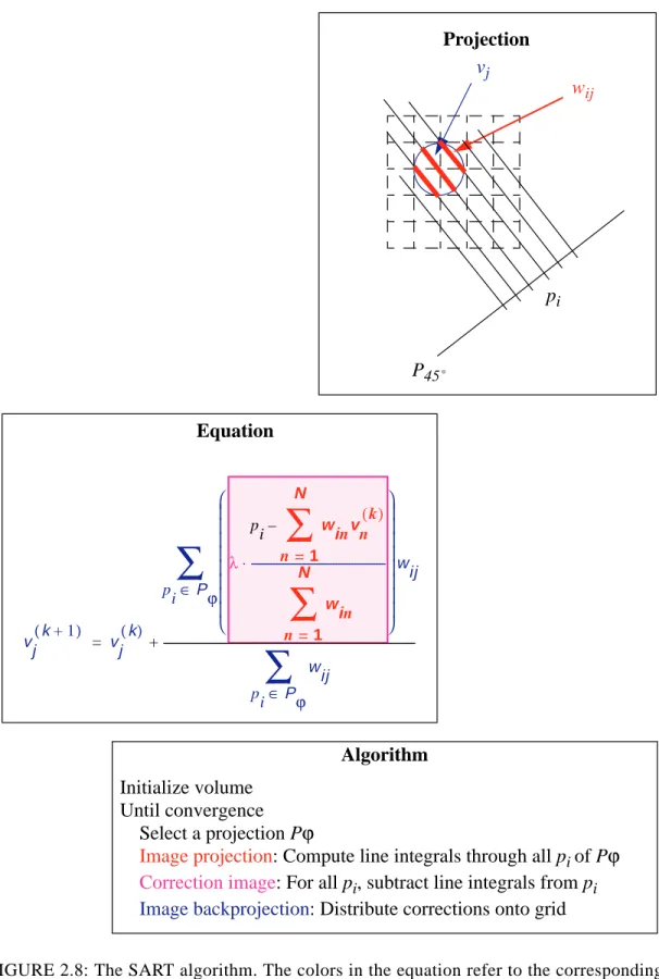
2.2 Simultaneous ART (SART) ... 28

2.3 Other Algebraic Reconstruction Methods ... 29

3. A GLOBALLY OPTIMIZING PROJECTION ACCESS ALGORITHM... 32

3.1 Introduction... 32

3.2 Previous Work... 33

3.3 The Weighted Distance Projection Ordering Scheme... 34

3.4 Results... 37

4. CONE-BEAM RECONSTRUCTION WITH ART: ACCURACY ISSUES... 44

4.1 Modified ART for Accurate Cone-Beam Reconstruction... 44

4.1.1 Reconstruction artifacts in traditional cone-beam ART ...46

4.1.2 New scheme for projection/backprojection to prevent reconstruction artifacts ...47

4.1.2.1 Adapting the projection algorithm for cone-beam ART...48

4.1.2.2 Adapting the backprojection algorithm for cone-beam ART ...53

4.1.2.3 Putting everything together...56

4.2 3D Cone-Beam Reconstruction with SART ... 59

4.3 Results... 60

4.4 Error Analysis ... 67

5. CONE-BEAM RECONSTRUCTION WITH ART: SPEED ISSUES... 69

5.1 Previous Work... 70

5.2 An Accurate Voxel-Driven Splatting Algorithm for Cone-Beam ART... 71

5.3 A Fast and Accurate Ray-Driven Splatting Algorithm for Cone-Beam ART... 73

5.3.1 Ray-Driven Splatting with Constant-Size Interpolation Kernels ...73

5.3.2 Ray-Driven Splatting with Variable-Size Interpolation Kernels ...75

5.4 Caching Schemes for Faster Execution of ART and SART ... 78

5.6 Cost and Feasibility of Algebraic Methods: Final Analysis ... 81

5.7 Error Analysis of Westover-Type Splatting ... 82

5.7.1 Errors from non-perpendicular traversal of the footprint polygon ... 82

5.7.2 Errors from non-perpendicular alignment of footprint polygon... 83

6. RAPID ART BY GRAPHICS HARDWARE ACCELERATION ... 87

6.1 Hardware Accelerated Projection/Backprojection... 88

6.2 Potential for Other Hardware Acceleration ... 92

6.2.1 Accumulation of the projection image ...94

6.2.2 Computation of the correction image ...96

6.2.3 Volume update ... 96

6.3 Optimal Memory Access ... 98

6.4 Increasing the Resolution of the Framebuffer ...100

6.4.1 Enhancing the framebuffer precision ... 101

6.4.2 A high precision accumulation framebuffer... 102

6.5 Results...103

6.6 Future Work - Parallel Implementations...105

7. CONCLUSIONS... 107

LIST OF TABLES

Table Page

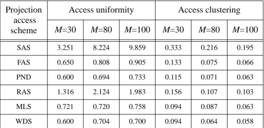
3.1 Projection access orders for all six ordering schemes (M=30) ... 38 3.2 Standard deviations of box counts for three projection set magnitudes

(M=30, 80, and 100) to measure projection access uniformity and

clustering ... 40 4.1 The definition of our 3D extension of the Shepp-Logan phantom ... 45 5.1 Run-times for SART, using both voxel-driven and ray-driven splatting, and

for ART using ray-driven splatting 80

6.1 Data structures of ART and TMA-ART and their pixel value ranges ... 92 6.2 Time performance of cone-beam TMA-ART for the different constituents

(tasks) of the program flow chart given in Figure 6.5 103 6.3 Runtimes per iteration for different enhancements of TMA-ART ...104

LIST OF FIGURES

Figure Page

1.1 Dynamic Spatial Reconstructor (DSR) ... 2

1.2 Biplane C-arm X-ray scanner . ... 4

1.3 Volumetric scanning geometries ... 6

1.4 Fourier Slice Theorem and Radon transform ... 7

1.5 Fan-beam geometric arrangement ... 8

1.6 Cone-beam source orbits ... 10

2.1 A beam bi due to ray r_i passes through projection image Pϕ... 16

2.2 Interpolation of a ray sample value s_ik ... 17

2.3 A ray r_i at orientationϕ enters the kernel of voxel v_j ... 18

2.4 Some interpolation filters in the spatial and in the frequency domain... 19

2.5 Interpolation of a discrete signal in the frequency domain ... 24

2.6 The ART algorithm ... 24

2.7 Kaczmarz’ iterative procedure for solving systems of linear equations ... 25

2.8 The SART algorithm ... 30

3.1 Projection order permutationτ for M=30 projections ... 34

3.2 Pseudo-code to illustrate insertion/removal of projections into/from circular queueΘ and listΛ... 35

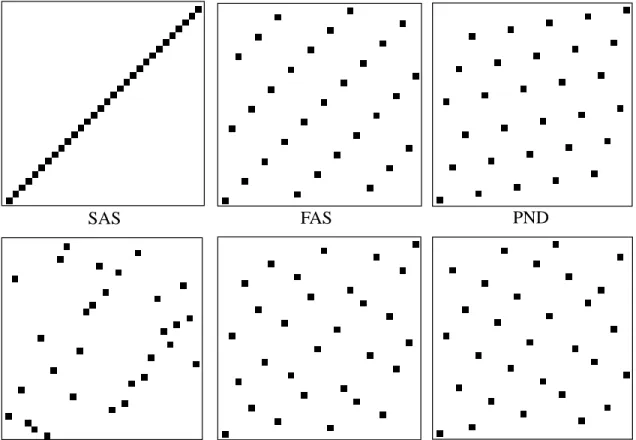
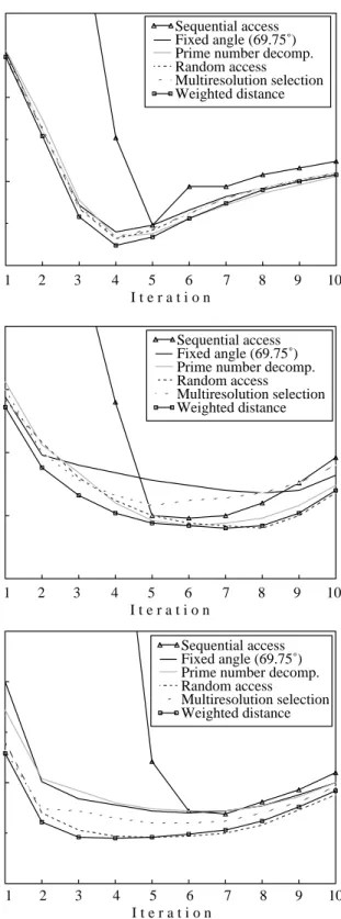
3.3 Sampling patterns in projection access space ... 39 3.4 Reconstruction errors for Shepp-Logan phantom for the six projection

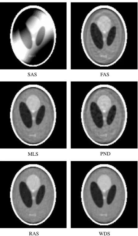
access schemes ... 41 3.5 Original 2D Shepp-Logan phantom ... 42 3.6 Reconstruction of the Shepp-Logan phantom after 3 iterations for the six

projection access schemes ... 43 4.1 Slices across the 3D Shepp-Logan brain phantom ... 46 4.2 The slices of Figure 4.1a reconstructed with traditional ART from

cone-beam projection data ... 47 4.3 Reconstruction of a solid sphere after one correction atϕ=0˚ was applied ... 48 4.4 Perspective projection for the 2D case ... 50 4.5 Frequency response and impulse response of the interpolation filter H’

and the combined filter HB 52

4.6 Grid projection at different slice depths in the frequency domain ... 54 4.7 Backprojection at different slice depths in the frequency domain ... 57 4.8 Reconstruction with ART utilizing the new variable-width interpolation

kernels ... 58 4.9 Reconstructing a uniform discrete correction signal c_s(z) into the

continuous signal c(z) with ART and SART using a linear interpolation

filter h ... 60 4.10 Reconstruction with SART .. ... 61 4.11 Correlation Coefficient (CC) and Background Coefficient of Variation

(CV) for ART and SART with constant and variable interpolation

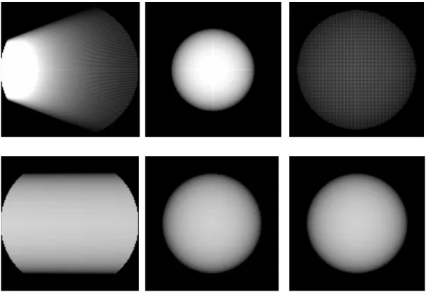
kernel size for 3 regions of the Sheph-Logan phantom 63 4.12 Reconstructions of the 3D Shepp-Logan brain phantom for cone angles of

20˚, 40˚, and 60˚ with different ART and SART parameter seetings ... 65 4.13 Computing the perpendicular ray distance to estimate the accurate ray grid

4.14 Shape of the rayfront with constant ... 68

4.15 The relative error e_stretch when using T_r instead of for stretching the kernel functions 68 5.1 Perspective voxel-driven splatting ... 72

5.2 Ray-driven splatting ... 74

5.3 Determining the local sampling rate of the arrangement of diverging rays ... 77

5.4 Error for different schemes of measuring the ray grid sampling rate ... 78

5.5 Errors from non-perpendicular traversal of footprint polygon ... 83

5.6 Errors from the non-perpendicular alignment of the footprint polygon ... 84

5.7 The angleϕ_cas a function of boundary voxel location on the reconstruction circle ... 85

5.8 Maximum normalized absolute error that occurs due to non-perpendicular alignment of the footprint polygons ... 86

6.1 Grid projection with TMA-ART... 88

6.2 Backprojection with TMA-ART ... 89

6.3 Stages of vertex transformation ... 90

6.4 Texture mapping an image onto a polygon ... 91

6.5 Flow chart of TMA-ART ... 93

6.6 Rendering a full 12bit data word into a 12bit framebuffer ... 95

6.7 Rendering a 12bit data word using 2 color channels ... 95

6.8 Hardware implementation of the volume update ... 97

6.9 Memory access order for different projection anglesϕ... 98

6.10 Voxels stored in x-y-z order ... 99 ω

r

ˆ

6.11 Voxels stored in y-x-z order ...100 6.12 Increasing the framebuffer resolution from 12 bit to 16 bit by adding up

two color channels, properly shifted 101

6.13 Accumulation framebuffer with 16 bit precision ...102 6.14 3D Shepp-Logan brain phantom reconstructed with both basic TMA-ART

CHAPTER 1

INTRODUCTION

There is no doubt that G.N. Hounsfield’s invention of the Computed Tomography (CT) scanner in 1972 has revolutionized diagnostic medicine. This invention has not only gained Hounsfield the honors of British Knighthood and the Nobel Prize in Medicine in 1979, but has also brought millions of dollars to the manufacturing company EMI, Ltd. and to others that have licensed the patent. But most importantly, it has, for the first time, made it possi-ble to visually inspect a person’s inside anatomy without the need for invasive surgery. Hounsfield’s invention showed that it was principally feasible, based on a very large num-ber of measurements, to reconstruct a cross-sectional slice of a patient with fairly high accuracy. In the following years, the image quality of the slices improved drastically. Two main reconstruction techniques emerged, which still exist up to this day: On one side there is the domain of direct methods that capitalize on the Fourier Slice Theorem [4], while on the other side lies the domain of iterative methods that seek to solve the reconstruction problem by solving a system of simultaneous linear equations. The most prominent mem-ber of the former group is the Filtered Backprojection (FBP) algorithm [5][50]. Here, the reconstruction is achieved by filtering the projection images with a ramp filter in frequency space, and then backprojecting the filtered projections onto a reconstruction grid. The first and still most prevalent representative of the iterative methods is the Algebraic Reconstruc-tion Technique (ART), attributed to Gordon et. al. [17]. Here, an object is reconstructed on a discrete grid by a sequence of alternating grid projections and correction backprojections. The projection measures how close the current state of the reconstructed object matches one of the scanner projections, while in the backprojection step a corrective factor is dis-tributed back onto the grid. Many such projection/backprojection operations are typically needed to make the reconstructed object fit all projections in the acquired set, within a cer-tain tolerance margin.

While two-dimensional (2D) slice-based CT has been in clinical use for many years, the current trend is now to three-dimensional (3D) or volumetric CT, in which projection acquisition is directly geared towards a 3D reconstruction of the object. This is in contrast to 3D representations obtained with standard slice-based CT, in which a number of

sepa-rately acquired, thin axial slices are simply stacked on top of one another.

One of the remaining great challenges in CT (and also other imaging modalities, like Mag-netic Spin Resonance (MRI)) is the 3D reconstruction of moving objects, such as the beat-ing heart, along with the coronary vessels and valves, and the lungs. Although these organs move in a cyclic fashion, they do so in slightly varying trajectories. Respiratory motion of the patient also contributes to this spatial variation. By gating image acquisition with a physiological signal, such as the ECG, one can tag the acquired images and associate them with a particular time instance within the organ’s cycle. In this way, images of equal time instances can be collected into a set and used for the 3D reconstruction of the object at that particular time frame. One can so generate animated, four-dimensional (4D) reconstruc-tions of the object, with the fourth dimension being time. However, the irregularity of the cycle trajectory causes inconsistencies within the images of a time set, since these images have not really been acquired at the same time instance, but only at equivalent time instances, a few cycles apart. This registration error will manifest itself in the reconstruc-tions as blurring and streaking.

The ultimate device to conduct this kind of dynamic imaging is the Dynamic Spatial Reconstructor (DSR), built as early as 1983 at the Mayo Clinic by Richard Robb [53][54] (shown in Figure 1.1). Here, 14 rotating 2D cameras with 240 scan lines each receive pho-tons of 14 opposing X-ray point sources at a frequency of 1/60 seconds. Thus, if a recon-struction algorithm requires, say 42 images, for faithful reconrecon-struction, and the imaged organ does not move much within this window of 4/60 seconds, then we can reconstruct this organ without the multi-cycle motion artifacts mentioned above, at a temporal resolu-tion of 4/60 seconds. There are, however, a few problems with the DSR: First, the scanner is very expensive, due to the replicated X-ray tubes and detectors, the heavy machinery required to rotate the gantry, and the electronics required to control image acquisition. Sec-ond, the gantry rotates only 1.5˚ per 1/60 sec, which means that the images per time window are not uniformly distributed in orientation angle. Hence, gated imaging is still necessary, although over a much reduced number of heart cycles.

FIGURE 1.1: Dynamic Spatial Reconstructor (DSR) built in 1983 at Mayo Clinic, Rochester, MN. (Image was obtained from http://everest.radiology.uiowa.edu/gallery/dsr.html).

At the time the DSR was developed, 3D reconstruction was still in its infancy and no true 3D reconstruction algorithm was available. In need of pioneering results, the DSR was forced to employ a standard 2D reconstruction algorithm, originally designed to reconstruct cross-sectional slices from fan-beam projection data. In an approach termed the stack-of-fans method, the DSR simply treated each axial row of projection data as coming from a rotating virtual 2D fan-beam source, located in the same plane. This approximation yielded reasonable results, which was not surprising since the source-detector distance (i.e., the gantry diameter) was quite large, reducing the subtended angle of the X-ray cone to a mere 4˚. Hence, the fans in the stack-of-fans were nearly parallel. A modern 3D scanner, how-ever, would employ much larger cone angles for the following reasons:

• smaller scanner design,

• to increase the utilization of the radially emitted X-rays, • better magnification,

• to expand the reach in the axial direction, and • to accommodate larger detector arrays.

As a matter of fact, micro-tomography (e.g., used to investigate the progress of osteoporo-sis in trabecular bone) uses cone-angles of up to 60˚. It should also be noted at this point that the DSR has never been duplicated, and rumor has it that it is currently being disman-tled for scrap.

If dynamic imaging is to be performed in a widespread clinical setting, it is probably more economical to resort to imaging equipment that is readily available at hospitals, such as a biplane C-arm X-ray scanner [11] (shown in Figure 1.2) or a standard CT-gantry with an added 2D camera [47][48][60] (similar to the DSR, just with one camera instead of 14). While the latter still requires modification of standard hospital equipment, however, at a smaller cost than the DSR, the former is available ready-to-go in great abundance.

Just to illustrate the efficacy of the former solution, let me give an example: The gantry of a standard biplane C-arm scanner rotates at maximal speeds of 10˚/s around the patient and acquires images at 30 frames/s per camera. With the biplane setup, we only need a little more than one quarter spin to cover the necessary angular range of about 220˚. Thus, with an acquisition time of 11s, we obtain 660 images (with the two cameras). If we were to image a patients heart, perfused with contrast dye, we would cover 11 patient heart beats (assuming the heart rate is the standard 1bps) with this amount of image data. If we then divided a heart beat into 15 time slots (like the DSR), we would have 44 images per time slot, fairly uniformly distributed over the semi-circle. Although workable, this is not overly generous, and we would need a reconstruction algorithm that can deal with this reduced amount of projection data.

Finally, yet another possible application of CT that has come into the spotlight is intra-oper-ative CT. Here, a patient undergoing a critical surgical procedure, such as a cerebral tumor ablation or a soft biopsy, is repeatedly imaged to verify the current status of the surgery. In contrast to intra-operative MRI, intra-operative CT does not require special non-magnetic instruments or electro-magnetic shielding. It is also much faster in the image generation

process (and less expensive). However, it does object patient and personnel to radiation. Hence, it is crucial to choose both a CT modality and a reconstruction algorithm that min-imize the number of acquired images and the amount of radiation dose that is needed to generate them.

This dissertation seeks to advance the field with these apparent challenges in mind. A pre-liminary goal can be stated as follows:

Devise a reconstruction framework that can faithfully and efficiently reconstruct a general volumetric object given a minimal number of projections images acquired in an efficient manner.

In order to zero in on this preliminary goal, two main decisions had to be made: • how are the object projections obtained, and

• what fundamental technique is used to reconstruct the object from these projections. In both categories there are several alternatives to choose from. The next section will expand on these alternatives and justify my choice — cone-beam acquisition with algebraic reconstruction. Then, in the following section, I will present the scientific contributions of this dissertation.

1.1 Methods for CT Data Acquisition and Reconstruction

This section discusses the currently available CT-based volumetric data acquisition meth-ods and will also expand on the two main suites of reconstruction algorithms, i.e., FBP and the algebraic techniques. The discussion concludes with the most favorable acquisition method and reconstruction technique to fulfill the preliminary goal stated above. First, I will enumerate the currently available volumetric CT imaging modalities.

1.1.1 Volumetric CT data acquisition techniques

For many years, the standard method of acquiring a volumetric CT scan has been by

ning a patient one slice at a time. In this method, a linear detector array and a X-ray point source are mounted across from each other. A fan-shaped X-ray beam (such as the one shown in Figure 1.3a) traverses the patient, and the attenuated fan is stored as a 1D linear image. By spinning the source/detector pair around the patient, a series of linear images is obtained which are subsequently used for 2D slice reconstruction. A volumetric represen-tation is obtained by advancing the table on which the patient rests after every spin, acquir-ing a stack of such slices. The problem with this approach is three-fold:

• Projection data covering patient regions between the thin slice sections is not avail-able, which can be a problem if a tumor is located right between two slices.

• The stop-and-go table movement may cause patient displacement between subsequent slice-scans, leading to slice-misalignment in the volume.

• A volumetric scan usually takes a long time, much longer than a single breath hold, due to the setup time prior to each slice acquisition. This introduces respiratory motion artifacts into the data, another source for data inconsistency.

The first two shortcomings have been eliminated with the recent introduction of the spiral (or helical) CT scanning devices (see Figure 1.3a). Again, one works with a linear detector array, but this time the patient table is translated continuously during the scan. Special reconstruction algorithms have been designed to produce a volumetric reconstruction based on the spiral projection data [9][27]. Although spiral CT is clearly a tremendous progress for volumetric CT, some problems still remain:

• Respiratory patient motion may still cause inconsistencies in the data set. Although the volumetric scans are obtained 5 to 8 times faster than with slice-based CT, they may still take longer than a patient’s breath hold.

• The emitted X-rays that fan out in a cone-shape are still under-utilized, since there is only one (or, in the more recent models, a few) linear detector array(s) that receive them. Those rays that are not used for image formation and just die out in the periph-ery unnecessarily contribute to the patient dose.

• 1D image data coming from the same gantry orientation, but from a different coil of the helix, are not temporally related. This makes it difficult to set up a protocol for gated imaging of moving physiological structures.

The final method leads us back to the old DSR, or better, its predecessor, the SSDSR (Sin-gle Source DSR), which adhered to the cone-beam imaging paradigm (shown in Figure 1.3). In cone-beam CT, a whole 3D dataset is acquired within only one spin around the patient. This provides for fast acquisition and better X-ray utilization, as this time a com-plete 2D detector array receives the cone-shaped flux of rays. The circumstance that all image data in a 2D image now originate from the same time instance enables easy gated imaging, and also provides an opportunity to use image-based methods for 3D reconstruc-tion.

1.1.2 Methods to reconstruct an object from its projections

In this section, I will discuss both FBP and algebraic methods in terms of their accuracy and computational cost. I will also give a brief description of both methods.

1.1.2.1 Brief description and cost of algebraic methods

A short description of the workings of algebraic methods has already been given in the beginning of this introduction. There, I mentioned that in algebraic methods an object is reconstructed by a sequence of alternating grid projections and correction backprojections. These projections and backprojections are executed for all M images in the acquired set, and possibly for many iterations I. Hence, the complexity of algebraic methods is mainly defined by the effort needed for grid projection and backprojection, multiplied by the num-ber of iterations. Since the effort for projection and backprojection is similar, we can write the cost of algebraic methods as:

(1.1)

We will see the reasoning behind the second form of this equation later. For now, consider a_Alg=1.

(a) (b)

FIGURE 1.3: Volumetric scanning geometries. (a) Spiral (helical) scan: the source and a 1D detector array are mounted opposite to each other and rotate in a spiral fashion many times around the patient. (b) Cone-beam scan: the source and a 2D detector array are mounted oppo-site to each other and rotate around the patient once.

Cost Algebraic( ) = 2 I M Cost Projection⋅ ⋅ ⋅ ( ) 2 a⋅ _Alg⋅ ⋅I M Cost Projection⋅ ( ) =

1.1.2.2 Description and cost of Filtered Backprojection

The Filtered Backprojection approach is a direct method and capitalizes on the Fourier Slice Theorem [4] and the Radon transform [30] (see Figure 1.4). The Radon transform of a 2D function f(x,y) is the line integral

(1.2) Thus a value at location s in a projection image g_θ(s) is given by integrating the object along a line perpendicular to the image plane oriented at angleθ. The Fourier Slice Theorem then states that the Fourier Transform (FT) of this projection image g_θ(s) is a line G_θ(ρ) in the frequency domain, oriented at angleθ and passing through the origin.

Obtaining a number of projections at uniformly spaced orientations and Fourier transform-ing them yields a polar grid of slices in the frequency domain (shown as the dashed lines in Figure 1.4b). However, we cannot simply interpolate this polar grid into a cartesian grid and then perform an inverse Fourier transform to reconstruct the object, as is explained as follows. The 2D inverse FT (IFT) f(x,y) of a signal F(u,v) is given by:

(1.3) g_θ( )s =

∫∫

f x y( , ) δ(xcosθ+ysinθ–s)dxdy θ x y g_ϕ(s) s u v G_θ(ρ)

(a) Spatial domain (b) Frequency domain

FIGURE 1.4: Fourier Slice Theorem and Radon transform

s

f(x,y F(u,v)

f x y( , ) =

∫∫

F u v( , )exp[i2π(ux+vy)]dudv

θ F(ρ θ, )exp[i2πρ(xcosθ+ysinθ)] ρdρ

0 ∞

∫

d 0 2π

∫

=

θ G(ρ θ, ) exp[i2πρ(xcosθ+ysinθ)] ρ dρ

∞ – ∞

∫

d 0 2π

∫

=

The first representation is the cartesian form, the second and third is the polar form. The last from of the equation states that an object given by f(x,y) can be reconstructed by scaling the polar slices G_θ(ρ) by |ρ|, performing a 1D IFT on them (inner integral), and finally backprojecting (=”smearing”) them onto the grid (outer integral). Thus we need 2 1D FT’s, the multiplications with |ρ|, and the backprojection step. Alternatively, one can convolve the g_θ(R) by the IFT of |ρ| and backproject that onto the grid. Note, that the IFT of |ρ| does not exist, but approximations (using large sinc-type filters) usually suffice. The former method is referred to as Filtered Backprojection (FBP), the latter as Convolution Back-projection (CBP).

So far, the discussion was restricted to the 2D parallel beam case. However, as was men-tioned in the previous section, modern slice-based CT scanners use the fan-beam approach, in which a point source with opposing 1D detector array are both mounted onto a rotating gantry. The (still experimental) cone-beam scanners extend the 1D linear detector array to a 2D detector matrix.

The good news is that the FBP and CBP algorithms can still be used, but with certain alter-ations, and, in the case of cone-beam, with certain restrictions. The diverging-beam case can be converted into the parallel-beam case by transforming the projection data as follows (see Figure 1.5).

First, one must move g_ϕ(s) to the origin, scaling the projection coordinates by s=s’(d/d’). Then, we must adjust the projection values for the path length difference due to the diverg-ing beams by multiplydiverg-ing each by the term . In the case of cone-beam, we just need to consider the t coordinate as well. After the data adjustment is performed, we

y x s’ d’ d central ray g_θ(s’) θ

FIGURE 1.5: Fan-beam geometric arrangement

filter by |ρ| as usual. Due to the diverging beam geometry, the backprojection is not simply a smearing action, but must be performed as a weighted backprojection. In the following discussion, consider the 3D cone-beam case which is the most general. Even though back-projection is done in a cartesian coordinate system, our data are still in a projective coordi-nate system, spanned by the image coordicoordi-nates s, t and the ray coordicoordi-nate r, given by the projected length of the ray onto the central ray, normalized by d. The mapping of this pro-jective coordinate system (s,t,r) to (x,y,z) is (rs,rt,r). This gives rise to the volumetric dif-ferential dx·dy·dz=r2ds·dt·dr. Thus, when backprojecting the projective data onto the cartesian grid, we must weight the contribution by 1/r2. The weighted backprojection inte-gral is then written as:

(1.4)

In the fan-beam case, given a sufficient number of projection images (see below), an object can be reconstructed with good accuracy. The cone-beam case is, however, more difficult. Here, certain criteria with respect to the orbit of the source detector pair have to be observed. A fundamental rule for faithful cone-beam reconstruction was formulated by Tuy and can be stated as follows:

Tuy’s Data Sufficiency Condition: For every plane that intersects the object, there must exist at least one cone-beam source point [64].

If this condition is not warranted, certain parts of the object will be suppressed or appear faded or blurred. Rizo et.al. give a good explanation for this behavior [52]. Tuy’s condition is clearly not satisfied by a single circular-orbit data acquisition (shown in Figure 1.6a). A possible remedy to this problem is to use two orthogonal circular orbits (one about the z-axis and one about the x-z-axis, for example) and merge the two projection sets. Note, how-ever, that this is not always feasible. Another way of satisfying the source-orbit criterion is to scan the object in a circular orbit as usual, but supplement this scan by a vertical scan without orbital motion. This acquisition path was advocated by Zeng and Gullberg [70] and is shown in Figure 1.6b. Other trajectories have also been proposed, such as a helical scan [65] or a circular orbit with a sinusoidal variation.

Prior to a cone-beam reconstruction with the modified parallel-beam reconstruction algo-rithm described above, we must filter the projection images in the Fourier domain (or alter-natively, convolve them in the spatial domain). If we choose to filter in the Fourier domain, we must transform and inversely transform the projection data. This is most efficiently done with a 2D FFT (Fast Fourier Transform) algorithm. The 2D FFT has a complexity of O(n2·log(n)), where n2 is the number of pixels in a projection image. Filtering G_θ(ρ) with a ramp filter has a complexity of O(n2). Thus the resulting actual cost for the entire filtering operation (2 FFTs and the pixel-wise multiplication by |ρ|) is somewhat lower than the cost for a projection operation (which has a complexity of O(n3)). However, a precise statement cannot be made, since we do not exactly know the constants involved in the O-notation. For now, we write the cost for FBP as:

f x y z( , , ) 1 r2 ----g s t( , ,θ) θd 0 π

∫

=

(1.5)

Here, a_FBP is a factor less than 1.0. It reflects the fact that filtering is probably less expen-sive than grid projection.

1.1.3 Preliminary comparison of FBP and algebraic methods in terms of

cost

Using equations (1.1) and (1.5), we can compare FBP and algebraic reconstruction in terms of their computational costs:

(1.6)

Clearly, if M_Alg=M_FBP and a_Alg=1, algebraic methods are bound to be much slower than FBP, even when I=1. However, I have distinguished M_Alg and M_FBP for a reason. As was shown by Guan and Gordon in [19], theoretically M_Alg<M_FBP, or to be more precise, M_Alg=M_FBP/2. In addition, one could imagine that some of the calculations done for grid projection could be reused for the subsequent grid backprojections. This would render a_Alg<1. Taking all this into account, we may be able to afford a number of iterations I>1, and still be competitive with FBP. In this respect, things don’t look all that bad for the alge-braic methods from the standpoint of computational cost.

FIGURE 1.6: Cone-beam source orbits: (a) single circular orbit, (b) circle-and-line orbit

(a) (b)

Cost FBP( ) = M⋅ (Cost Projection( ) +Cost Filtering( )) 1+a_FBP ( ) ⋅M Cost Projection⋅ ( ) = Cost Algebraic( ) Cost FBP( ) --- 2 a⋅ Alg⋅I⋅MAlg 1+a_FBP ( ) ⋅M_FBP ---=

1.1.4 Comparison of FBP and algebraic methods in terms of quality

Let me now consider the two methods in terms of their reconstruction quality. In clinical, slice-based CT, FBP is nowadays exclusively used. This due to the computational advan-tages that I have outlined in the previous paragraphs. Note, however, that clinical CT scan-ners usually acquire more than 500 line projections per slice, which approximates the continuous form of the inverse Radon integral rather well. The true power of algebraic methods is revealed in cases where one does not have a large set of projections available, when the projections are not distributed uniformly in angle, when the projections are sparse or missing at certain orientations, or when one wants to model some of the photon scatter-ing artifacts in the reconstruction procedure [1][30][36]. Noise as present in many clinical CT datasets is also better handled by algebraic methods [30], a fact that has been discovered by researchers in PET (Positron Emission Tomography) and SPECT (Single Photon Emis-sion Computed Tomography) imaging as well [35][55]. Finally, algebraic methods allow a-priory constraints to be applied onto the shape or density of the reconstructed object, before and during the reconstruction process. In this way, the reconstruction can be influ-enced and guided to produce an object of better contrast and delineation than it would have without such intervention [60].

While 2D fan-beam tomographic reconstruction has been routinely used for over two decades, 3D cone-beam reconstruction is still in the research stage. As yet, there are no clin-ical cone-beam scanners, however, there are a number of experimental setups at academic institutions [11][47][48][60] and corporate labs (Hitachi, GE, Siemens, and Elscint). A variety of cone-beam algorithms based on FBP have also been proposed. The most notable ones are Feldkamp, Davis, and Kress [12], Grangeat [15], and Smith [59], all published in the mid and late 1980s. While the research on general 2D algebraic methods [17][19][23][25] and 2D fan-beam algebraic methods [22][36] is numerous, the published literature on 3D reconstructors using algebraic algorithms is rather sparse. One exception is the work by Matej et. al. [35], whose studies in the field of fully-3D reconstruction of noisy PET data indicate that ART, produces quantitatively better reconstruction results than the more popular FBP and MLE (Maximum Likelihood Estimation) methods. In this case, however, not a cone-beam reconstructor was used, but the projection rays were re-binned which simplified ART to the parallel-beam case. Another group of researchers has successfully applied ART for SPECT data [55] not long ago. Again, no cone-beam recon-struction was performed, rather, the data were rebinned for parallel-beam reconrecon-struction. However, the most popular use of 3D cone-beam ART is in 3D computed angiography. As was already touched on in a previous section of this introduction, in computed angiography one acquires images of blood-perfused structures injected with radio-opaque dye while rotating the cone-beam X-ray source-detector pair around the patient. For toxicity reasons, the dye injection time is limited and thus the number of projections that can be acquired is restricted as well. Computed angiography is a prime candidate for ART, as its projection data feature many of the insufficiencies that were noted above as being better handled by ART (as opposed to FBP): Only a limited amount of projection data is available, the pro-jections are not necessarily taken at equi-distant angles, and the propro-jections are usually

noisy. In addition, one can often improve the appearance and detail of the reconstructed vessels by isolating the vessels from the background after a couple of iterations, and just use these segmented volume regions in the remaining iterations [60]. For example, Ning and Rooker [47] and Saint-Felix et. al. [60] all use ART-type methods to 3D reconstruct vascular trees in the head and abdominal regions. One should keep in mind, however, that the objects reconstructed in 3D computed angiography are of rather high contrast, which poses the reconstruction problem as almost a binary one. To a lesser degree, this is also true for PET and SPECT reconstructions.

It were the promising reported qualitative advantages of algebraic methods in the limited projection data case, its better noise tolerance, and the lack of any fundamental research on algebraic methods in the up-and-coming field of general, low-contrast cone-beam recon-struction, that led me to dedicate this dissertational research to the advancement of alge-braic methods in this setting. In the following, I shall give an outlook on the several scientific contributions that were achieved in the course of this endeavour.

1.2 Contributions of this Dissertation

In this dissertation, I have undertaken and accomplished the task of advancing the current state of the “ART” to a more general arena than high-contrast computed angiography. I have conceived algorithms that produce accurate 3D reconstructions for cone angles as wide as 60˚ and object contrasts as low as 0.5%. This just about covers the range of all cone-beam reconstruction tasks, in-vivo and in-vitro, from clinical CT to micro-tomography of biological specimen.

However, having designed a highly accurate reconstruction algorithm is only half of the story. In order to make it applicable in a clinical setting, it is also important that this algo-rithm produces its results in a reasonable amount of time. When this dissertation work was begun, algebraic methods were nowhere near this premise. As indicated by equation (1.6), algebraic methods have two main variables that can be attacked for this purpose:

• the number of iterations needed to converge to a solution that fits a certain conver-gence criterion, and

• the complexity of the projection/backprojection operations.

This dissertation provides solutions that seek to minimize both of these crucial variables, without sacrificing reconstruction quality.

Finally, with a growing number of graphics workstations being introduced in hospitals for visualization purposes, the idea is not far-fetched to use these same workstations also for 3D reconstruction of these datasets. This would lead to a better utilization of these work-stations, and would certainly be a more economical solution than to build or purchase spe-cial reconstruction hardware boards. Since algebraic reconstruction mostly consists of projection/backprojection operations, a task at which these workstations are really good at, one can expect great computational speedups when porting algebraic algorithms to utilize this hardware. The final chapter of this dissertation will report on such an attempt, which

led to a speedup of over 75 compared to the software implementation, at only little decline in reconstruction quality.

Hence, the final goal of this dissertation can be defined as follows:

Extend the existing theory of algebraic methods into the previously unexplored domain of general, low-contrast cone-beam reconstruction. Devise techniques that provide reconstructions of high quality at low computational effort, with the ultimate aim of making ART an efficient choice for routine clinical use.

CHAPTER 2

ALGEBRAIC METHODS:

BACKGROUND

In this chapter, the principles of algebraic methods will be described. First, I will discuss the Algebraic Reconstruction Technique (ART) [17], which is the oldest method of this kind. Then I will turn to a related method, Simultaneous ART (SART), developed later by Anderson and Kak [2] as a means to suppress noise in the reconstructions. Although this dissertation will be confined to these two variants of algebraic methods, others exist that will be briefly discussed in the final section of this chapter.

2.1 The Algebraic Reconstruction Technique (ART)

The Algebraic Reconstruction Technique (ART) was proposed by Gordon, Bender, and Herman in [17] as a method for the reconstruction of three-dimensional objects from elec-tron-microscopic scans and X-ray photography. This seminal work was a major break-through, as the Fourier methods that existed in those days were highly limited in the scope of objects that they were able to reconstruct, and, in addition, were also rather wasteful in terms of their computational requirements. It is generally believed that it was ART that Hounsfield used in his first generation of CT scanners. However, as we also know, the Fou-rier methods matured quickly and captured ART’s territory soon after.

Let me now describe the theory of ART as relevant for this dissertation. Although ART, in its original form, was proposed to reconstruct 3D objects, it represented them as a stack of separately reconstructed 2D slices, in a parallel beam geometry. For the remaining discus-sion, I will extend the original 2D notation into 3D, which is more convenient considering the scope of this dissertation. The extension is trivial, and can always be reduced to the 2D case.

2.1.1 ART as a system of linear equations

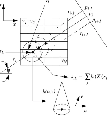
ART can be written as a linear algebra problem: WV=P. Here, V is the unknown (N×1) col-umn vector storing the values of all N=n3 volume elements or voxels in the n × n×n recon-struction grid. P is the (R×1) column vector, composed of the R=M·R_m values of the pixels p_i in the combined set of all M projection images P_ϕ of R_m picture elements or pixels each, where the P_ϕ are the images obtained from the imaging device at angles ϕ of the X-ray detector plane (see Figure 2.1). Finally, W is the (R×N) weight (or coefficient) matrix in which an element w_ijrepresents a measure of the influence that voxel v_j has on the ray r_i passing through pixel p_i. We can write WV=P in an expanded form as a system of linear equations:

(2.1)

It is clear that the weight coefficients bear a crucial role in the solution of this equation sys-tem. They are the elements that link the unknown voxel values to the known pixel values. For the solution to be accurate, each weight w_ij must accurately represent the influence of a voxel v_j on a ray r_i passing through pixel p_i. The first ART incarnation by Gordon, Bender, and Herman [17] represented a voxel grid by a raster of squares (see Figure 2.1). A weight w_ij was set to 1 if a ray r_i passed through the square of voxel v_j and was set to 0 otherwise. Later, Shepp and Logan [61] computed the actual area of intersection of the ray beam that is bounded by the rays emanated from the pixel boundaries on the image plane. It is this approach that is shown in Figure 2.1. In many current ART implementations the ray beam is reduced back to a thin linear ray r_i. However, this time a coefficient w_ij is deter-mined by the length of r_i in voxel v_j. Herman et. al. have shown in their software package SNARK [24], that the calculation of the w_ij along r_i requires only a few additions per voxel and can be done very efficiently using an incremental Digital Differential Analyzer (DDA) algorithm (see [13]). All these implementations represent a voxel by a square (or a cubic box in 3D), which is a rather crude approximation, according to well-known principles of sampling theory [49]. The following section will expand on this issue and conclude with a voxel basis that is more appropriate than the box.

2.1.2 Choosing a good voxel basis

Consider again Figure 2.1. Here, we see that, although the originally imaged object was continuous, i.e., each point in space had a defined density value, the reconstruction only yields a discrete approximation of this object on a discrete raster. However, in contrast to the representation of Figure 2.1, this raster does not consist of equi-valued tiles, which would mean that the reconstructed object is a granulated representation of itself. Rather, it is a raster of lines in which the known values, or grid samples, are only explicitly given at

w₁₁v₁+w₁₂v₂+w₁₃v₃+…+w_1Nv_N = p₁ w₂₁v₁+w₂₂v₂+w₂₃v₃+…+w_2Nv_N = p₂

…

the intersection of the raster lines, also called grid points. Object values at volume locations other than the grid points can be obtained by a process called interpolation. Hence, a con-tinuous description of the object could (theoretically) be reconstructed by performing these interpolations everywhere in the volume. To see what is meant by interpolation, consider Figure 2.2. Here, a ray r_i is cast into the volume and samples the volume at equidistant points. Since not every point coincides with a grid point, a weighting function, represented by the interpolation kernel h(u,v), is centered at each sample point. The surrounding grid points that fall within the interpolation kernel’s extent are integrated, properly weighted by the interpolation kernel function (here a simple bilinear function). Figure 2.2 shows how a sample value s_ik at a ray sample position (X(s_ik),Y(s_ik)) is calculated from the neighboring voxels.

The value s_ik is given by:

(2.2) The entire ray sum for pixel p_i is then given by the sum of all s_ik along the ray r_i:

(2.3)

FIGURE 2.1: A beam b_i due to ray r_i passes through projection image P_ϕ at pixel p_i and sub-tends a voxel v_j. In early propositions of ART, a voxel v_jwas a block (square or cube) of uni-form density. A weight factor w_ij was computed as the subtended area normalized by the total voxel area. v₁ v_N v₂ v_j w_ij Area Area ---= p_i-1 p_i p_i+1 P_ϕ=70˚ r_i-1 r_i r_i+1 b_i-1 b_i b_i+1 s_ik h X s( ( )_ik –X v( )_j ,Y s( )_ik –Y v( )_j ) ⋅v_j j

∑

= p_i h X s( ( )_ik –X v( )_j ,Y s( )_ik –Y v( )_j ) ⋅v_j j

∑

k

∑

=

This ray sum is a discrete approximation of the ray integral:

(2.4)

We can reorder this equation into:

(2.5)

This is shown in Figure 2.3. We see the similarity to the equations in (2.1). Here, a pixel was given by:

(2.6) Hence, the weights are given by the integrals of the interpolation kernel along the ray:

(2.7) h(u,v) x y r_i r_i-1 r_i+1 p_i-1 p_i p_i+1 P_ϕ

FIGURE 2.2: Interpolation of a ray sample value s_ik located at (X(s_ik),Y(s_ik)) in the

reconstruc-tion grid. All those discrete reconstrucreconstruc-tion grid points v_jthat fall into the extent of interpola-tion kernel h(u,v) centered at (X(s_ik),Y(s_ik)) are properly weighted by the interpolation kernel

function at (X(s_ik)-X(v_j),Y(s_ik)-Y(v_j) and summed to form the value of sample s_ik of ray r_i.

s_ik h X s( ( )_ik –X v( )_j ,Y s( )_ik –Y v( )_j ) ⋅v_j j

∑

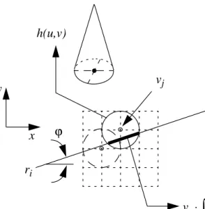
= u v v_j v₁ v₂ v_N s_k ϕ p_i h X s( ( )_i –X v( )_j ,Y s( )_i –Y v( )_j ) ⋅v_j j

∑

   ds_i

∫

= p_i v_j⋅

∫

h X s( ( )_i –X v( )_j ,Y s( )_i –Y v( )_j )ds_i j

∑

= p_i v_j⋅w_ij k

∑

= w_ij =

∫

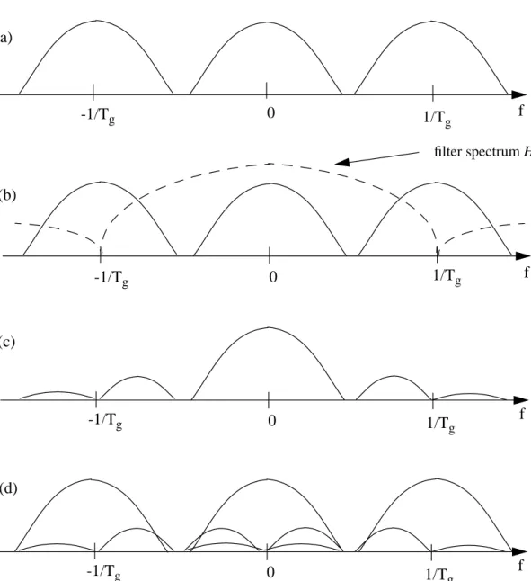
h X s( ( )_i –X v( )_j ,Y s( )_i –Y v( )_j )ds_i

Obviously, the better the interpolation kernel, the better the interpolation, and the more accurate the weight factor. Figure 2.4 shows some popular interpolation kernels, both in the spatial (Figure 2.4a) and in the frequency domain (Figure 2.4b). (We will return to these plots in a few paragraphs.) The frequency plot tells us how good a filter is. Generally, when reconstructing a function from discrete samples, we want the filter to have a high amplitude for frequencies < 0.5/T_g and a low amplitude for frequencies > 0.5/T_g,where 1/T_gis the grid sampling rate. We want that because discrete functions have their spectra replicated as aliases at multiples of 1/T_g, and reconstructing with an interpolation filter means multiply-ing the discrete signal’s frequency spectrum with the spectrum of the filter.

To clarify these statements, let me analyze the interpolation process a little more in detail. The interpolation of a sample value at any location in a discrete grid can be decomposed as follows:

• Reconstruction of the continuous function f from the discrete grid function f_s by con-volving f with the interpolation filter h.

• Resampling of the reconstructed continuous function f at the sample’s location

(X(s_ik),Y(s_ik)).

Consider now Figure 2.5a. Here, we see the frequency spectrum of the discrete grid signal, F_s. The spectrum has a main lobe centered at f=0, and aliases, replicated at a frequency of 1/T_g. When reconstructing f from f_s, we want to recover just the main lobe and none of the aliases. However, real-life interpolation filters will always include some of the aliases into

v_j h(u,v) r_i x y ϕ

FIGURE 2.3: A ray r_i at orientationϕ enters the kernel of voxel v_jand integrates it along its path.

0 0.2 0.4 0.6 0.8 1 1.2 1.4 1.6 1.8 2 −200 −180 −160 −140 −120 −100 −80 −60 −40 −20 0 Frequency Relative power (dB) Box Bilinear Gaussian Sinc Bessel−Kaiser −3 −2 −1 0 1 2 3 −0.4 −0.2 0 0.2 0.4 0.6 0.8 1 x Amplitude Box Bilinear Gaussian Sinc Bessel−Kaiser (a) (b)

FIGURE 2.4: Some interpolation filters: (a) spatial plots, (b) frequency plots.

r

-1/T_{g 1/Tg} 1/T_g -1/T_g 1/T_g -1/T_g 0 0 0 f f f (a) (b) (c)

FIGURE 2.5: Interpolation of a discrete signal (solid line), frequency domain: (a) Spectrum of the original discrete signal, F_s, replicas (aliases) of the signal spectrum are located at multiples of 1/T_g. (b) Multiplication with the spectrum of the (non-ideal) interpolation filter H. (c) Resulting frequency spectrum F of the interpolated signal. Note that some of the signal’s aliases survived due to the imperfect interpolation filter. (d) Re-sampled interpolated signal. The aliases in the signal replicas in the sidelobes show up in the main lobe. The composite sig-nal is irrecoverably distorted.

filter spectrum H

1/T_g

-1/T_g 0 f

the reconstructed function. Let me now illustrate what the decomposition of the interpola-tion process in the spatial domain, as shown above, translates to in the frequency domain:

• Reconstruction of f from f_s is equivalent to the multiplication of the discrete signals’s spectrum F_swith the spectrum of the interpolation filter, H. This process is shown in Figure 2.5b. Note the remaining (attenuated) signal aliases in F, shown in Figure 2.5c. These aliases have disturbing effects (such as ghosts and false edges) in f. (This form of aliasing is called post-aliasing).

• Resampling of f is equivalent to replicating the reconstructed spectrum F at a fre-quency 1/T_g. Note, in Figure 2.5d, that the attenuated signal aliases that survived the reconstruction process now reach into neighboring lobes in the new discrete signal. Thus, the re-sampled discrete signal has irrecoverable artifacts (called pre-aliasing). A far more detailed description of this process is given in [69]. Now, as we know more about the effect of a good interpolation filter, let me return to Figure 2.4. Here, we see a few interpolation filters, both in the spatial domain and in the frequency domain. The ideal interpolation filter is the sinc filter, as its box-shape in the frequency domain blocks off all signal aliases. The sinc filter passes all frequencies < 0.5·1/T_g (the passband) unattenuated, and it totally blocks off all frequencies > 0.5·1/T_g (the stopband). The sinc filter, however, has an infinite extent in the spatial domain, and is therefore impractical to use. On the other extreme is the box filter. It has an extent of 0.5 in the spatial domain, and has the worst performance in blocking off signal aliases in the stopband. It is that boxfilter that is used by the ART implementations mentioned before. We now easily recognize that this filter, although very efficient due to its small spatial extent, is probably not the best choice for reconstruction. Figure 2.4 also shows the frequency spectra and spatial waveforms of the bilinear filter, a Gaussian filter 2^(-4·r2), and a Bessel-Kaiser filter. The last two filters have a spatial extent of 4.0 and are also radially symmetric in higher dimensions. This will prove to be an advantage later.

The family of Bessel-Kaiser functions were investigated for higher dimensions by Lewitt in [32] and used (by the same author) for ART in [31] and [33]. The Bessel-Kaiser func-tions have several nice characteristics:

• They are tunable to assume many spatial shapes and frequency spectra. Consider again the frequency plots in Figure 2.4b. We observe that the spectrum of the Bessel-Kaiser function has a main-lobe that falls off to zero at the grid sampling frequencyω=1/T_g, and returns with many fast decaying side-lobes. The tuning parameters control the placement of the zero-minima between the mainlobe and the sidelobes. They also con-trol the rate of decay. Since the signal’s first sidelobe is at maximum at a frequency

ω=1/T_g,we would want to place the zero-minimum of the filter’s spectrum at that loca-tion for best anti-aliasing effects. The circumstance that the filter decays fast in the stopband suppresses all of the signal’s higher-order sidelobes to insignificance.

• Another characteristic of the Bessel-Kaiser function is that they have, in contrast to the Gaussian function, a finite spatial extent (here a radius of 2.0). Truncation effects, that possibly appear with a necessarily truncated Gaussian, are thus avoided.

• Finally, the Bessel-Kaiser function has a closed-form solution for the ray integration. Due to Lewitt’s convincing arguments, and also due to a very efficient implementation (described later), I have solely used Bessel-Kaiser functions as the voxel basis in the dis-sertational research presented here. However, it should be noted that other voxel bases have also been used in the past: Andersen and Kak represented a voxel by a bilinear kernel [2], and I (in [44]) chose a Gaussian kernel in the early days of this research.

For convenience and completeness, I shall repeat some of the results derived in [32] for the Bessel-Kaiser function in higher dimensions. First, the generalized Bessel-Kaiser function is defined in the spatial domain as follows:

(2.8)

Here, a determines the extent of the function (chosen to be 2.0), and α is the taper parameter that determines the trade-off between the width of the main lobe and the amplitude of the side lobes in the Fourier transform of the function. (Whenα=0, we get the box function of width 2a.) The function I_m() is the modified Bessel function of the first kind and order m. We set m=2 to get a continuous derivative at the kernel border and everywhere else in the kernel’s extent.

The corresponding Fourier transform is given as:

(2.9)

Here, n is the dimension of the function to be reconstructed. If we reconstruct 2D slices, n=2, for volumetric 3D reconstruction n=3. The function J_n/2+m() is the Bessel function of the first kind and order n/2+m. We see that, depending on n, different values ofα are nec-essary to place the zero-minimum between the filter’s mainlobe and its first sidelobe at

ω=1/T_g. We can calculate that for a 2D kernelα=10.80, and for a 3D kernelα=10.40. Finally, the Abel transform pm(r) (i.e., the X-ray projection) of the generalized Bessel-Kai-ser function b(m,α)(r) can be shown to be proportional to b(m + 1/2,α)(r):

(2.1