Three essays on financial economics

(1)

c

(2)

THREE ESSAYS ON FINANCIAL ECONOMICS

BY

LIFENG GU

DISSERTATION

Submitted in partial fulfillment of the requirements

for the degree of Doctor of Philosophy in Finance

in the Graduate College of the

University of Illinois at Urbana-Champaign, 2013

Urbana, Illinois

Doctoral Committee:

Associate Professor Dirk Hackbarth, Chair

Professor Timothy C Johnson

Professor George Pennacchi

(3)

Abstract

My first essay,

Product Market Competition,

R

&

D

Investment and Stock Returns, considers the

in-teraction between product market competition and investment in research and development (R&D)

to tackle two asset pricing puzzles: the positive R&D-return relation and the positive

competition-return relation. Using a standard model of R&D competition-return dynamics, I establish that competition and

R&D investments have a strong interaction effect on stock returns. It is more likely that firms with

high R&D expenditures will end up with very low returns on their ventures because rival firms

win the innovation race. Because there are more potential rival firms in competitive industries,

R&D intensive firms in competitive industries are riskier. Consistent with the predictions of the

model, I find a robust empirical relation between R&D intensity and stock returns, but only in

competitive industries. This finding suggests that the risk derived from product market

competi-tion has important asset pricing implicacompeti-tions and potentially drives a large porcompeti-tion of the positive

R&D-return relation. Furthermore, firms in competitive industries earn higher returns than firms

in concentrated industries only among R&D-intensive firms. My second finding therefore provides

a risk-based explanation for the heretofore puzzling competition premium.

The second essay,

Governance and Equity Prices: Does Transparency Matter?, examines how

a firm’s information environment and corporate governance interact. Firms with higher takeover

vulnerability are associated with higher abnormal returns, but even more so if they also have higher

accounting transparency. The effect is largely monotonic — it is small and insignificant for opaque

firms and large and significant for transparent firms — and it holds in sample splits based on

firm characteristics, such as leverage or size. A portfolio that buys firms with the highest level of

takeover vulnerability and shorts firms with the lowest level of takeover vulnerability — provided

it includes the tercile of transparent firms as defined by the first principal component of forecast

error, forecast dispersion, and revision volatility — generates a monthly abnormal return of 1.37%

for value-weighted (1.28% for equal-weighted) portfolios, which is nearly twice as large as the alpha

in the full sample. This result survives numerous robustness tests, and it also remains large and

significant even if we extend the sample period until 2006. Hence transparency and governance

(i.e., takeover vulnerability) are complements. This complementarity effect is consistent with the

view that more transparent firms are more likely to be taken over, since acquirers can bid more

effectively and identify synergies more precisely.

(4)

formation environment as additional predicting variable since a transparent environment could

facilitate takeovers by making it easier for bidders to value the firm and the synergy of the deal.

The logit estimation including this new variable over the sample period of 1991 to 2009 produces

results consistent with this view and better fits the real takeover data. The new takeover factor

constructed as the return to the long-short portfolio that buys firms with top takeover probability

and sells firms with bottom takeover probability better captures the variation in the cross-section

of stock returns.

(5)

(6)

Acknowledgments

I am very grateful to my adviser, Dirk Hackbarth, for his encouragement and guidance. Many

thanks to my committee members, Timothy Johnson, George Pennacchi, Prachi Deuskar for their

advise and support. Also I would like to thank all other members in the Department of Finance at

the University of Illinois at Urbana-Champaign for their assistance. Finally, special thanks to my

parents who have been providing me with love and support during this long journey.

(7)

Product Market Competition, R&D

Investment and Stock Returns

1.1 Introduction

Investment in research and development (R&D) is one of the crucial elements of corporate activities

that drive companies’ long-term viability. A large share of the US stock market consists of firms

that invest in R&D intensively. Often a firm enters into an innovation race with many rivals. If a

competitor successfully completes the project first, then other firms may have to suspend or even

abandon their projects. Because R&D investment tends to be irreversible, suspension or

abandon-ment of the R&D project significantly reduces firm value. Therefore, competition can have a large

impact on R&D-intensive firms.

Prior research in asset pricing has uncovered two asset pricing puzzles: the positive R&D-return

relation and the positive competition-return relation.

1

However, they have largely been regarded as

unrelated to each other, and we still lack a thorough understanding of the real mechanism driving

these two return patterns. Thus research on the interaction effect between R&D investment and

competition can shed new light on these two puzzles.

This paper studies the joint effect of product market competition and R&D investment on stock

returns. My analysis is based on a partial equilibrium model for a multi-stage R&D venture by

Berk, Green, and Naik (2004). Specifically, I establish two hypotheses: (1) The positive

R&D-return relation is stronger in competitive industries; (2) The positive competition-R&D-return relation

strengthens among R&D-intensive firms. In other words, there is a strong positive interaction effect

1_{The two asset pricing puzzles are the positive R&D-return relation (Chan, Lakonishok, and Sougiannis (2001))} and the competition premium (Hou and Robinson (2006)). In the literature of R&D investments and stock returns, researchers have proposed different ways to measure firms’ innovation activity such as R&D investments, R&D increment, R&D efficiency and R&D ability and consistently find positive premiums associated with those measures. However, we still lack a thorough understanding of the real mechanism driving this return pattern. Hou and Robinson (2006) show that firms in competitive industries outperform firms in concentrated industries. They speculate that this might be because either barriers to enter concentrated industries insulate firms from undiversifiable distress risk or concentrated industries are less innovative. However, so far no article has provided any formal tests or explanation to address the mechanism underlying the competition premium.

(10)

between competition and R&D investment on stock returns.

In the model, the firm progresses through the R&D project stage by stage and decides whether

to incur an instantaneous R&D investment to continue the project or not. Prior to completion,

the decision maker can observe the future cash flows that the project would be producing if it were

completed today. Since the risk associated with cash flows has a systematic component, this feature

imparts to the project a large amount of systematic risk, and the R&D venture can be considered

as a series of compound options on systematic uncertainty. Since options have higher systematic

risk than the underlying asset because of implicit leverage, the R&D venture demands a higher risk

premium than the stochastic cash flow itself.

Competition increases the probability that the potential future cash flows will be extinguished,

and thus decreases the benefit of investing and raises the chance of project suspension in the event

of an adverse shock to the future cash flow. Therefore, firms’ investment decisions and value are

more sensitive to the systematic risk that the cash flow carries. Moreover, this negative impact of

a potential extinguishing of cash flow is more pronounced for firms with high R&D inputs because

high R&D inputs further reduce the value of the option to invest. As a result, the model implies a

strong positive relation between competition and stock returns among R&D-intensive firms. It also

predicts a stronger positive relation between R&D investment and returns for firms surrounded by

high competition.

I test the model’s predictions empirically with firm-level data over the 1963 to 2009 period

and document a robust positive interaction effect between product market competition and R&D

investment on stock returns. Following the literature, I employ a Herfindahl (concentration) index

to gauge the competitiveness of an industry, and I use four alternative measures to proxy for firm’s

R&D intensity: R&D expenditure scaled by net sales, R&D expenditure scaled by total assets, R&D

expenditure scaled by capital expenditure, and R&D capital scaled by total assets. The purpose of

using different measures is to make sure that the results are not driven by the size effect. Following

Chan, Lakonishok, and Sougiannis (2001), I compute R&D capital as the sum of the depreciated

R&D expenditures over the past five years, assuming an annual depreciation rate of 20%.

First, I adopt the portfolio sorting approach to test the model’s predictions. Specifically, in

June of each year, firms are sorted independently into three groups (bottom 30%, middle 40%,

top 30%) based on the Herfindahl index and R&D intensity in the previous year.

2

The abnormal

returns to the resulting nine portfolios are computed adjusting for the Fama-French three-factor

model and the Carhart (1997) four-factor model.

My first finding is that the positive R&D-return relation only exists in competitive industries.

More precisely, the abnormal return to the double-sorted portfolio increases monotonically with

R&D intensity for firms in competitive industries, but this return pattern does not exist for firms

from concentrated industries. This finding holds for all four measures of R&D intensity, and for both

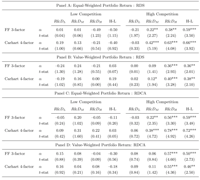
equal-weighted and value-weighted portfolio returns. For instance, when R&D intensity is measured

2_{Sorting on these two measures sequentially produces qualitatively and quantitatively similar or even stronger} results.

(11)

by R&D capital scaled by assets, in competitive industries, the monthly equal-weighted four-factor

abnormal returns for the low, medium, and high R&D intensity portfolios are 0.06%, 0.38%, and

0.78%, with

t-statistics of 0.72, 4.72 and 4.92, respectively. This results in a 72 basis points monthly

return difference between the high and low R&D intensity portfolios. In contrast, for concentrated

industries, the abnormal returns for the low, medium, and high R&D intensity portfolios are much

smaller and insignificant: they are 0.09%, 0.31%, and 0.22%, with

t-statistics of 0.42, 1.60 and 0.41,

respectively. This translates to a monthly return spread of 0.13% with a

t-statistic of 0.05.

My second finding is that the positive competition-return relation only exists among R&D

inten-sive firms. More specifically, the portfolio abnormal return increases monotonically with industry

competition level for firms with high R&D inputs, but this pattern does not exist for firms with low

R&D inputs. For example, when R&D intensity is measured by R&D expenditure scaled by sales,

for R&D-intensive firms, the monthly equal-weighted four-factor abnormal returns for the low,

medium, and high competition portfolios are –0.21%, 0.42%, and 0.63%, with

t-statistics of 0.54,

1.90 and 4.08, respectively. The monthly return difference between the high and low competition

portfolio is 0.84% with a statistical significance at 5% level. In contrast, for firms with low R&D

inputs, the abnormal returns of the competition portfolios are small and insignificant. The monthly

abnormal return spread between the high and low competition portfolio is –0.22% and insignificant.

The positive interaction effect between R&D intensity and product market competition is also

confirmed by the estimation results of Fama-MacBeth cross-sectional return regressions.

Specifi-cally, the coefficient on the interaction term,

R

&

D

∗

HHI

, is negative and significant at the 5%

level for all measures of R&D intensity.

3

For example, when R&D intensity is proxyed by R&D

expenditure scaled by sales, the slope on the interaction term is –1.15% and significant at the 5%

level. It is –1.08% and significant at the 5% level when R&D is measured by R&D capital scaled by

assets. Moreover, I perform the same tests using dummy variables instead of continuous variables

for R&D intensity and industry competition. I find that the coefficient on the interaction term for

R&D-intensive firms in competitive industries,

R

&

D

high

∗

HHI

low

, is always positive and

signif-icant, while the coefficient on other interaction terms is much smaller and insignificant in almost

all cases. For example, when R&D intensity is measured by R&D expenditure scaled by sales, the

coefficient on the interaction term,

R

&

D

high

∗

HHI

low

, is 0.42% and significant at the 1% level.

This is consistent with the portfolio sorting results that there is always a positive and significant

abnormal return associated with the portfolio of high R&D intensity and high competition.

My main findings survive numerous robustness tests. I re-estimate the

α

using alternative

as-set pricing models which are extensions of the Carhart (1997) four-factor model with additional

factors proposed in the literature, including the liquidity factor of Pastor and Stambaugh (2003);

the takeover factor of Cremers, John, and Nair (2009); and the misvaluation factor of Hirshleifer

and Jiang (2010). Interestingly, none of these factors weaken the abnormal returns, indicating

that liquidity, takeover probability and investor misvaluation are not the reasons driving the main

3_{Since high} _HHI _{index value means low competiton level, a negative sign shows a positive interaction effect} between R&D intensity and industry competition.

(12)

findings documented in this article.

In addition to these tests, I also experiment with dividing the full sample into

financial-constrained and financial-unfinancial-constrained subsamples or into high-innovation-ability or

low-innovation-ability subsamples to verify that the main result is not due to these two firm characteristics that

are identified to affect R&D investment’s risk or effectiveness. Li (2011) finds that the positive

return relation is driven by financial constraints. She documents that the positive

R&D-return relation exists only among financially constrained firms. I examine whether my results

are driven by financial constraints by dividing the full sample into financially-constrained and

financially-unconstrained subsamples. I find that the positive R&D-return relation is present for

both financially constrained and unconstrained firms, only if they are also from competitive

in-dustries. This finding indicates that financial constraints don’t seem to affect the R&D-return

relation once I control for competition. Cohen, Diether, and Malloy (2011) provide evidence that

R&D predicts future returns only when firms have high ability to translate the outcome of those

innovation projects into real sales growth. They document a significantly positive adjusted return

associated with

GOODR

&

D

(i.e., high R&D intensity and high ability) firms. I test whether my

results are driven by innovation ability by dividing the full sample into high-innovation-ability or

low-innovation-ability subsamples. The positive R&D-return relation exists for both subsamples,

but only when the firms are also from competitive industries. This result leads to another

interest-ing findinterest-ing that innovation ability does not seem to affect the R&D-return relation once I control

for competition. Overall, the main findings along with the results of these robustness tests show

that product market competition creates another important dimension that matters for the link

between R&D investment and stock returns.

I also investigate whether investor limited attention can explain my findings by dividing the

whole sample into subsamples based on firm size, firm analyst coverage, and firm idiosyncratic

volatility. The fact that my findings exist in all subsamples indicate that investor limited attention is

not the main driver. I further provide evidence in supportive of the risk hypothesis by showing that

the portfolio of R&D intensive firms in competitive industries are actually associated with higher

cash flow risk by examining the volatility of firm performance measures such as return on assets,

return on equity, and profit margin. Thus the test results indicate that the positive and significant

abnormal returns are driven by risk factors that are not captured by existing asset pricing models.

To further explore the asset pricing implications of firm innovation, I construct a new factor,

the innovation factor, following the procedure in Fama-French (1993) and Chen, Novy-Marx and

Zhang (2011). The innovation factor is formed as the weighted-average return of a zero-cost trading

strategy that takes a long position in stocks with high innovation levels and a short position in

stocks with low innovation levels. This strategy earns a significant average return of 37 basis points

per month over the sample period.

Furthermore, I test the performance of this innovation factor using the

competition-minus-concentration portfolio in Hou and Robinson (2006) who document that firms in competitive

in-dustries earn higher returns than firms in concentrated inin-dustries and this competition premium

(13)

persists after adjusting for common risk factors. Interestingly, augmenting the Carhart (1997)

four-factor model with the innovation factor brings the abnormal return of the

competition-minus-concentration hedge portfolio down to an insignificant level with a much smaller magnitude. This

finding therefore provides a risk-based explanation for the competition premium.

This article has two main contributions. First, it contributes to the literature on the relation

be-tween R&D investment and stock returns (e.g., Chan, Lakonishok, and Sougiannis 2001; Chambers,

Jennings, and Thompson 2002; Lin 2007; Li 2011; Cohen, Diether, and Malloy 2012). I show that

the positive R&D-return relation exists only for firms from competitive industries. This empirical

finding along with the implications developed from the model indicate that competition has a large

impact on the risk and return profiles of R&D-intensive firms and it potentially drives a large portion

of the positive R&D-return relation. Second, this article also contributes to the research on the

rela-tion between competirela-tion and stock returns. I document a robust empirical relarela-tion between

compe-tition and return, but only among firms with intensive R&D inputs. This suggests that firms

engag-ing in high levels of innovation activities in competitive industries are actually contributengag-ing to this

positive competition premium. Thus the finding in this article also provides a risk-based explanation

for the heretofore puzzling competition-return relation documented in Hou and Robinson (2006).

The rest of the paper is organized as follows. Section 2 contains the development of testable

hypotheses. Section 3 provides details of the data sources, sample selection, variable definitions.

Section 4 examines the joint effect of product market competition and R&D investments on stock

re-turns empirically. Main results, robustness checks and interpretations are presented in this section.

Finally, Section 5 concludes.

1.2 Hypotheses development

To study the interaction effect of industry competition and R&D investment on risk premium, I

adopt the model from Berk, Green, and Naik (2004), who develop a partial equilibrium model for

a single multi-stage R&D venture. I provide a brief overview of the model before I derive the two

testable hypotheses that I will test with the data in the empirical part of the paper.

1.2.1 Overview of the model

The firm operates in continuous time and progresses through the R&D project stage by stage. It

receives a stream of stochastic cash flows after it successfully completes

N

discrete stages. At any

point in time prior to completion, the manager has to make investment decisions to maximize the

firm’s intrinsic value. Before proceeding to the valuation details of the R&D venture, I discuss

several important model assumptions:

1. An important feature of the model is that it assumes the decision maker can observe the future

cash flow the project would be producing were it complete today and the decision to continue

the project is made based on this information. Therefore the systematic risk of the future cash

(14)

flow is imparted to firm’s investment decisions. Thus the R&D project can be considered as a

series of compound options on the underlying cash flows which have systematic uncertainty.

Since options have higher systematic risk than the underlying asset because of implicit

lever-age, the R&D venture demands a higher risk premium than the stochastic cash flow itself.

Take gold mining as an concrete example. The successes and failures in gold mining sites will

average out when the company has thousands of mining sites in different locations. Often

this type of “geological risks” are taken as diversifiable in textbooks. However, the decision

to continue mining at any particular site is made with the current price of gold in mind.

2. Success intensity

π

(

n

(

t

)): The number of completed stages at time

t

is denoted by

n

(

t

).

At any point in time prior to completion, the firm must make R&D investment decisions.

Conditional on investment, the probability that the firm will complete the current stage and

advance to the next stage in the next instant is

πdt

.

π

is the success intensity. In the

sim-plified case in Berk, Green, and Naik (2004)’s model,

π

is a known function of

n

(

t

). For

simplicity, I assume it as a constant over all stages. Thus, I write it as

π

hereafter.

3. Investment cost

RD

(

n

(

t

)): If the firm decides to continue the project, it has to incur an

investment cost. The R&D cost can be a known function of the number of completed stages

n

(

t

). For simplicity, I set it as a constant over all stages. Thus, I write it as

RD

hereafter.

Note that the investment level is not a choice variable.

4. Competition or obsolescence risk: It is assumed that the fixed probability that the potential

or actual cash flow is extinguished over the next instant is

φdt

.

φ

is the obsolescence rate. In

the model, this risk is idiosyncratic and does not demand any risk premium itself. However,

a high probability of obsolescence indicates that it is more likely that the potential cash flows

will become zero. Thus a high obsolescence rate lowers the benefit of investing and the value

of the option to continue the project. Therefore, it affects the firm’s decision to continue or

suspend the project and thus indirectly its systematic risk and risk premium.

1.2.2 Valuation

After the firm successfully completes

N

discrete stages, it receives a stream of stochastic cash flow,

c

(

t

), which follows a geometric Brownian motion:

dc

(

t

) =

µc

(

t

)

dt

+

σc

(

t

)

dw

(

t

)

,

(1.1)

where

µ

is the constant growth rate of cash flows,

σ

is the constant standard deviation of cash

flows, and

dw

(

t

) is an increment of a Wiener process.

The partial equilibrium model adopts an exogenous pricing kernel, which is given by the

fol-lowing process

(15)

where

r

is the constant risk-free rate and the risk premium for the cash flow process

c

(

t

) is denoted

as

λ

=

σθρ,

(1.3)

where

ρ

is the correlation between the Brownian motion processes

w

(

t

) and

z

(

t

).

Under the risk-neutral measure, the cash flow process

c

(

t

) follows a geometric Brownian motion:

dc

(

t

) = ˆ

µc

(

t

)

dt

+

σc

(

t

)

d

w

ˆ

(

t

)

,

(1.4)

where ˆ

w

(

t

) is a Brownian motion under the risk-neutral measure and ˆ

µ

=

µ

−

λ

is the constant

drift term of the cash flow process under the risk-neutral measure.

Upon making decisions about whether to continue investing or not, the firm’s manager

ob-serves (1) the number of completed stages,

n

(

t

); (2) the level of cash flow the project would be

producing were the project complete already; and (3) whether the firm’s potential cash flows have

been extinguished through obsolescence. Note that both success intensity

π

and investment cost

RD

are assumed to be known functions of

n

(

t

). If the cash flow is extinguished, the firm value

becomes zero. Thus conditional on the project being alive, the firm value at time

t

depends on the

future cash flow,

c

(

t

), and the number of completed stages,

n

(

t

). It is denoted by

V

(

c

(

t

)

, n

(

t

)). For

simplicity, I write it as

V

(

c, n

) hereafter.

If the project is completed successfully, the firm receives a stream of stochastic cash flows. Thus

at that point the firm value is simply the continuous-time version of the Gordon-Williams growth

model. At any time

t

prior to the completion of the project, the firm value is the maximum of

the firm’s risk-neutral expected discounted future value at time

T

(

T

is an arbitrary point in the

future) plus the discounted value of any cash flows received from time

t

to

T

. This multi-stage

investment problem is given as

V

(

c, n

) =

max

u(s)∈{0,1},s∈(t,T)

E

Q t

[ ] is the expectation operator under the risk-neutral (pricing) measure,

Q

.

ν

is an indicator variable, taking value of 0 or 1 to keep track of whether the project is completed

or not (

ν

= 1 indicates that the project is completed and

n

(

t

) =

N

.

ν

= 0 indicates that the

project is not completed and

n

(

t

)

< N

.).

RD

is the instantaneous R&D cost if the firm continues

investing over the next instant. Note that the level of the R&D investment is not a choice variable.

φ

is the obsolescence rate; that is, the probability of the occurrence of an obsolescence event

which could result in zero future cash flows in the next instant. In competitive industries, many

firms are competing in the development of a new product or technology. Once one firm claims

victory, it will take the cash flows produced by the new product and other firms face a project with

zero future cash flows and thus have to restructure or abandon the R&D project. In contrast, in

non-competitive industries, there are fewer competitors and firms can conduct the development with less

(16)

fear about the breakthrough of rivals. Therefore,

φ

will tend to be higher in competitive industries.

By applying Ito’s lemma to the value function

V

(

c, n

) we can derive the

Hamilton-Bellman-Jacobi equation of the investment problem. It is given as follows:

(

r

+

φ

)

V

(

c, n

) =

1

2 σ

2

_c

2

∂

2

∂c

2

V

(

c, n

) + ˆ

µc

∂

∂c

V

(

c, n

) + max

u∈{0,1}

uπ

[

V

(

c, n

+ 1)

−

V

(

c, n

)]

−

RD,

(1.6)

where

π

denotes the probability that the firm will successfully complete the current stage over the

next instant if the firm invests. Once it successfully advances to the next stage, the firm value

will jump to

V

(

c, n

+ 1). Thus,

π

[

V

(

c, n

+ 1)

−

V

(

c, n

)] is the expected jump in firm value after

the investment or the benefit of investing. Consider a biotechnology firm as an example. Its value

usually jumps after the firm advances to more advanced phases.

At each instant of time, the firm makes an investment decision. If future cash flow exceeds a

threshold

c

∗

(

n

) which is determined by the fundamentals, the firm will invest and

u

= 1. If future

cash flow is below the threshold

c

∗

(

n

), the firm will suspend the project and

u

= 0. These two

regions are denoted as the “continuation” and “mothball” regions, respectively. The analytical

solution of the above Hamilton-Bellman-Jacobi equation can be derived by specifying its function

form in both continuation and mothball regions and applying standard boundary conditions at the

cash flow threshold. Berk, Green, and Naik (2004) provides detailed derivations, and I reproduce

them in Appendix A for reference.

Following standard arguments (i.e., Itˆ

o

’s Lemma), the risk premium of the R&D venture at

stage

n

,

R

(

n

), can be derived as follows

R

(

n

) =

(

∂V

(

c, n

)

/∂c

)

c

V

(

c, n

)

λ

(1.7)

After the project is completed, no further investment decision is needed and the venture is

equivalent to a traditional cash producing project which demands the same risk premium

λ

as the

stochastic cash flow process. Before completion, in the mothball region, the firm is equivalent to

an option to invest. This is riskier than the underlying cash flow because of the implicit leverage

feature of options. In the continuation region, the firm consists of an option to suspend, the

dis-counted value of future cash flow, and the expected R&D cost. Thus the firm in the continuation

region is less risky than the mothball region and riskier than the underlying cash flow. In the

following subsections, I develop hypotheses that show how a R&D firm’s risk premium

R

(

n

) varies

with its investment level

RD

and the obsolescence rate

φ

.

1.2.3 R&D investment and risk premium

At any point in time prior to completion, the firm has to make an investment decision. If future

cash flow is below a threshold, the firm will suspend the project. A firm that needs to overcome

a higher cash flow threshold in order to continue the project is riskier because a high cash flow

threshold increases the chance of project suspension in the event of an adverse shock to future cash

(17)

flow. Therefore, the firm’s investment decision and value are more sensitive to the systematic risk

the cash flow carries.

A higher R&D investment requirement tends to lower the value of the option to continue the

project and thus raises the cash flow threshold the firm needs to overcome. Therefore, a higher R&D

investment requirement leads to a higher risk premium. In other words, firms with intensive R&D

investments have high expected returns. Furthermore, this positive relation is stronger for firms

from industries with high obsolescence rates (i.e., competitive industries) because a high

obsoles-cence rate further raises the cash flow threshold and R&D-intensive firm’s investment decisions and

value are more sensitive to the systematic risk the cash flow carries. A high obsolescence rate leads

to a high probability of cash flow extinguishing and thus lowers the benefit of continuing the R&D

investment. Therefore, the obsolescence rate is positively associated with the cash flow threshold.

The above insight yields the first hypothesis.

4

Hypothesis 1.

In the continuation region where cash flow

c >

=

c

∗

(

n

),

∂R

(

n

)

∂RD

>

0 (1.8)

∂

2

R

(

n

)

∂RD∂φ

>

0 (1.9)

To have a visual understanding of these effects, I numerically show these relations with a R&D

venture which needs five stages to complete. I adopt the same parameter values as in Berk, Green,

and Naik (2004), which are as follows: the risk-free rate

r

is 7% per year. The drift

µ

and the

standard deviation

σ

of the cash flow process is 3% and 40%, respectively. The risk premium for

the cash flow process

λ

is 8% per year. The success intensity

π

is set as a constant throughout

all stages of the venture for simplicity.

5

_{The value is 2.0, which is equivalent to 86% probability}

of successfully completing one stage in a year.

6

The absolesence rate

φ

ranges from 0.05 to 0.25

cross-sectionally.

7

The required R&D investment is set to be a constant throughout all five stages.

It is 5.0 for firms with low R&D inputs and 25.0 for firms with high R&D inputs.

8

4

These properties are not proved analytically. I show these properties using numerical examples.

5_{The results are robust to how the success intensity varies with each additional completed stage. For example,} in one of the unreported cases, I set the value ofπin an increasing manner. That is, it starts with a low value and increases by 0.2 as the project advances to the next stage. The results still hold.

6

IfN(t) denotes the number of events that occurred before timetand follows the possion distribution, then the probability that there arekevents occurred during the time interval [t, t+τ] isP[N(t+τ)−N(t) =k] = e−λτ_k(_!λτ)k. ThusP[N(t+τ)−N(t)>0] = 1−e−λτ. Letτ = 1 andλ= 2, then the probability of completing at least one stage in a year is 1−e−2_{= 0}_._86.

7

IfN(t) denotes the number of events that occurred before timetand follows the possion distribution, then the probability that there arekevents occurred during the time interval [t, t+τ] isP[N(t+τ)−N(t) =k] = e−λτ_k(_!λτ)k. Thus P[N(t+τ)−N(t) = 0] = e−λτ_{. Let} _τ _{= 1 and} _λ ₌_φ_{, then the probability of surviving one year without}

obolescence ise−φ. The range ofφfrom 0.05 to 0.25 corresponds to a surviving probability range from 0.77 to 0.95. 8

R&D reporting firms are sorted into quintile portfolios based on their R&D intensites measured by R&D expen-ditures scaled by assets. The mean value of R&D intensity is 0.01 in the lowest qunintile and 0.24 in the highest quintine. In the model, we can obtain a variable which is equivalent to this R&D intensity by using the required R&D investments scaled by firm value averaged across all stages of the project. Whenφis 0.1 and the future cash

(18)

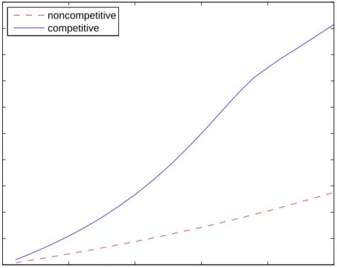
Figure 1.1 plots firms’ risk premium

R

(

n

) against their R&D investment requirements

RD

for

different levels of obsolescence rates (i.e., different levels of competition) and for different stages

prior to the completion of the project. The horizontal parts in the plot correspond to the mothball

regions where the cash flow is below the threshold. As is shown in the plots, R&D investment is

positively related to the risk premium in the continuation regions. This is true for all stages of the

R&D venture. Moreover, this positive R&D-return relation is stronger for firms from competitive

industries (i.e., industries with higher obsolescence rates). In addition, this positive relation

weak-ens as the project gets closer to completion. As is shown in the bottom right plot when

n

= 4, the

magnitude of the risk premium is much smaller than that in earlier stages. This is because firm’s

value increases as more stages are completed and this reduces the chance of project suspension.

The same intuition is illustrated in Figure 1.2 where the risk premium is computed by averaging

it over all stages of the project. All parameter values are the same as in Figure 1.1. As is displayed,

the risk premium increases with the level of R&D investment requirement and this positive

rela-tion is stronger for firms operating in competitive industries. The indicarela-tions of this hypothesis is

consistent with the empirical findings in the second part of this paper.

1.2.4 Competition and risk premium

A high obsolescence rate leads to a high probability that the potential or actual future cash flow

will be extinguished and thus lowers the benefit of continuing the R&D investment. Therefore,

firms in industries with higher obsolescence rates (i.e., competitive industries) need to pass higher

cash flow thresholds to continue the project and thus have higher risk premium. In other words,

firms from competitive industries have higher expected returns. In addition, this positive relation

is stronger among firms with intensive R&D inputs which are also positively associated with the

cash flow thresholds. This insight yields the second hypothesis.

9

Hypothesis 2.

In the continuation region where cash flow

c >

=

c

∗

(

n

),

∂R

(

n

)

∂φ

>

0 (1.10)

∂

2

R

(

n

)

∂φ∂RD

>

0 (1.11)

Similarly, I use numerical examples to illustrate the properties stated in the above hypothesis.

Figure 1.3 plots firms’ risk premiums against the obsolescence rates (or levels of competition) for

different levels of R&D investment requirements and for different stages. It can be seen clearly that

the positive competition-return relation prevails in each subplot of the figure and the relation is

more pronounced among firms with intensive R&D investments.

and 25, respectively.

9_{Equation (11) in hypothesis 2 is the same as Equation (9) in Hypothesis 1 in terms of mathematics. I put the} same equation in two different hypotheses because there are two relations in the paper: the R&D-return relation and the competition-return relation and I want to illustrate the properties of these two relations separately.

(19)

Figure 1.4 shows the same intuition by plotting the risk premium averaged over different stages

against the obsolescence rate. As is shown, the positive relation between competition and the risk

premium manifests among firms with high R&D inputs. The indications of this hypothesis is also

consistent with the empirical findings.

Figure 1.5 and Figure 1.6 illustrate the relations between risk premium and R&D investment

and obsolescence rate in integrated three-dimensional plots. Figure 1.5 provides subplots for

dif-ferent stages and Figure 1.6 uses the risk premium averaged across difdif-ferent stages. As is shown,

the risk premium increases as R&D investment requirement and obsolescence rate increases. The

flat parts in the plot are the mothball regions where cash flow is lower than the threshold. Similar

pattern can be found in Figure 1.6.

To check whether the risk premium patterns in the numerical examples still hold with different

parameter values, I vary the value of the parameters in the model by 50% and find consistent

results. In Figure 1.7 and Figure 1.8, I show the plots for two cases: the volatility of the cash flow

process,

σ

, and the success intensity,

π

.

10

These are key variables that have large impact on the

value of the option to invest and hence firm’s investment decisions and demanded risk premium.

In the original exercise,

σ

is set to 40% and

π

is set to be 2.0. In Figure 1.7, I show the numerical

results when

σ

is set to 0.2 and 0.6, respectively. In Figure 1.8, I present the numerical results

when

π

is set to 1.0 and 3.0, respectively.

11

In both figures I show the relations between the risk

premium averaged across all stages and R&D investment requirement (

RD

) and competition level

(obsolescence rate,

φ

) in 3D plots. As is displayed, the plots in Figure 1.7 and Figure 1.8 show

similar risk premium patterns as the plot in Figure 1.6.

In sum, the hypotheses that the positive R&D-return relation prevails in competitive industries

and that the positive competition-return relation is stronger among R&D-intensive firms follow

directly from the Berk, Green, and Naik’s (2004) framework for analyzing R&D return dynamics.

Next, I turn to test the above hypotheses with a variety of empirical methods.

1.3 Data

1.3.1 Sample Selection and Definition of Variables

My main data sources are from the Center for Research in Security Prices (CRSP) and

COMPUS-TAT Annual Industrial Files from 1963 to 2009. I obtain firms’ monthly stock returns from CRSP

and firms’ accounting information from COMPUSTAT. To be included in the sample, the firm

must have a match in both data sets. Following Fama and French (1992), only NYSE, AMEX-,

and NASDAQ-listed securities with share codes 10 and 11 are included in the sample. That is, only

firms with ordinary common equity are included (ADRs, REITs, and units of beneficial interest

are excluded). Finally, firms in financial and regulated industries are excluded.

10_{The results are robust when I vary the value of other parameters.} 11

The assumption, π = 1, corresponds to a 63% probability of completing at least one stage in a year. π = 3, corresponds to a 95% probability of completing at least one stage in a year.

(20)

To ensure that the accounting information is already incorporated into stock returns, I follow

Fama and French (1992) to match accounting information for all fiscal year ends in calendar year

t−

1 with CRSP stock return data from July of year

t

to June of year

t

+1. So there is a minimum half

a year gap between fiscal year end and the stock return, which provides a certain period of time for

the accounting information to be impounded into stock prices. However, firms have different fiscal

year ends and thus the time gap between the accounting data and matching stock returns varies

across firms. In order to check if this matching procedure biases the main results, I also perform

the tests using the sample of firms with December fiscal year ends and similar results are obtained.

Product market competition is measured by Herfindahl index (HHI), a measure commonly used

by researchers in the literature of industrial organization.

12

It is defined as the sum of squared

market shares

HHI

jt

=

Nj

X

i=1

s

2_ijt

(1.12)

where

s

ijt

is the market share of firm

i

in industry

j

in year

t

,

N

j

is the number of firms in industry

j

in year

t

, and

HHI

jt

is the Herfindahl index of industry

j

in year

t

. Market share of an individual

firm is calculated by using firm’s net sales (COMPUSTAT item #12) divided by the total sales

value of the whole industry.

13

Following Hou and Robinson (2006), I classify industries with

three-digit SIC code from CRSP and all firms with non-missing sales value are included in the sample to

calculate the Herfindahl index for a particular industry.

14

The calculation is performed every year

and the average values over the past three years is used in the analysis as the Herfindahl index of

an industry to prevent potential data errors.

15

Throughout the paper four measures of R&D intensity are employed to proxy for firm’s

in-novation level: R&D expenditure scaled by total assets (

RDA

), R&D expenditure scaled by net

sales (

RDS

), R&D expenditure scaled by capital expenditure (

RDCAP

), and R&D capital scaled

by total assets (

RDCA

).

16

Following Chan, Lakonishok, and Sougiannis (2001), I compute the

R&D capital assuming an annual depreciation rate of 20% over the past five years. Specifically, the

equation is as follows:

(1.13)

where

RDC

it

is the R&D capital for firm

i

in year

t

and

RD

it−j

is the R&D expenditure

j

years

ago. Although the R&D intensity measures are constructed differently, they are highly correlated

with each other. For example, the correlation between

RDS

and

RDCA

is 0.73.

12

See, e.g., Hou and Robinson (2006), Giroud and Mueller (2011). The use of Herfindahl index to measure product market competition is also supported by the theory. See Tirole(1988), pp221-223.

13

Using the same procedure, the Herfindahl index can be constructed using firms’ assets or equity data. These alternative measures produce qualitatively similar test results.

14

On the one hand, extremely fine industry classification will result in statistically unreliable portfolios. On the other hand, if the classification is not fine enough, firms in different business line will be grouped together.

15

This averaging procedure is also used in Hou and Robinson (2006). 16

These measures are commonly used in the literature of innovation. See, e.g., Lev and Sougiannis (1996, 1999), Li (2011), Cohen, Diether, and Malloy (2011).

(21)

1.4 Results

Before testing the main hypotheses, I first replicate the empirical results documented in two

sem-inal papers: Hou and Robinson (2006) and Chan, Lakonishok, and Sougiannis (2001). Hou and

Robinson (2006) find that firms in competitive industries earn higher abnormal returns than firms

in concentrated industries over the sample period of 1963 to 2001. Chan, Lakonishok, and

Sougian-nis (2001) show that firms conducting intensive R&D activities are associated with higher stock

returns over the period of 1975 to 1995. I extend the sample period to 2009 and re-examine these

two empirical relations by using portfolio sorting approach.

First I replicate the positive R&D-return relation. In June of each year

t

, firms are sorted into

quintile portfolios based on their value of R&D capital scaled by total assets in year

t

−

1.

17

Then

time-series regression of excess monthly portfolio return on risk factors is performed using

Fama-French three-factor model and Carhart (1997) four-factor model. In particular, the Fama-Fama-French

three-factor model is estimated in the following equation

R

t

=

α

+

t

(1.14)

and the Carhart (1997) four-factor model is estimated as

R

t

=

α

is the value-weighted

mar-ket return minus the risk free rate in month

t

,

SM B

t

is the month

t

size factor,

HM L

t

is the

book-to-market factor in month

t

, and

U M D

t

is the month

t

Carhart momentum factor.

RM RF

t

,

SM B

t

, and

HM L

t

factors are downloaded from Kenneth French’s website and the

U M D

t

factor

is constructed according to Carhart (1997).

Panel A and Panel B in Table 1.1 report the intercept

α

of the estimation. Both equal-weighted

and value-weighted portfolio results are presented. When computing value-weighted return, I use

the market capitalization from previous month as the weight. Consistent with Chan, Lakonishok,

and Sougiannis (2001) and other studies (e.g., Li (2011), Hirshleifer, Hsu, and Li (2011), Cohen,

Diether, and Malloy(2011)), I find the abnormal returns increase monotonically from the lowest

R&D intensity portfolio (Quintile 1) to the highest R&D intensity portfolio (Quintile 5). More

specifically, in Panel A, for the equal-weighted portfolio, the monthly three-factor

α

is –0.03%

(t–statistic = 0.28) for quintile 1, it is 0.16% (t–statistic = 1.68) for quintile 3, and it is 0.56%

(t–statistic = 2.95) for quintile 5. The return spread between quintile 1 and quintile 5 is 59 basis

points per month (t–statistic = 3.02). Similarly, in Panel B, using the Carhart (1997) four-factor

model, the return spread between the lowest and highest R&D intensity quintile portfolio grows to

70 basis points per month and it is statistically significant (t–statistic = 3.59).

Next I turn to the analysis of the positive competition-return relation. In June of each year

t

,

(22)

firms are grouped into quintile portfolios according to their value of Herfindahl index in year

t−

1. I

estimate the abnormal return

α

by running time-series regression of excess monthly portfolio return

on common risk factors. Panel C and Panel D report the results for Fama-French three-factor model

and Carhart (1997) four-factor model, respectively. As is shown, firms in competitive industries earn

higher abnormal returns, while firms in concentrated industries earn lower abnormal returns. The

abnormal return decreases almost monotonically as the competition level decreases from quintile

1 to quintile 5.

18

Specifically, in Panel D, the value-weighted four-factor

α

is 0.06% (t–statistic =

1.91) for the lowest quintile and it decreases to –0.18% (t–statistic = 1.54) for the highest quintile.

The abnormal return difference between the highest and lowest quintiles is –0.24% per month and

it is statistically significant (t–statistic = 1.91). However, the equal-weighted return spreads are

not significant, although the return pattern across the quintiles does show that firms in competitive

industries outperform firms in concentrated industries. All in all, the replication results largely

confirm that the finding in Hou and Robinson (2006) is still valid with extended sample period.

In sum, the above analysis not only confirms that the two important empirical results

docu-mented in the literature survive in an extended sample period, but also indicates that these risk

premiums can not be explained by existing common risk factors such as the market factor, the

size factor, the value factor and the momentum factor.

The model predicts that the positive

R&D-return relation strengthens with the level of competition and the positive competition-return

relation strengthens with firm’s R&D intensity. That is, there is a strong positive interaction

ef-fect between R&D intensity and product market competition. In the rest of the paper, I focus on

studying this interaction effect from empirical perspectives.

1.4.1 Interaction between R&D Intensity and Product Market Competition

In this section, I investigate the positive interaction effect between production market competition

and firm R&D intensity using portfolio analysis and Fama-MacBeth cross-sectional regressions.

Portfolio Analysis

First I study the interaction effect using a conventional double sorting approach. Specifically, in

June of each year

t

, NYSE, Amex, and NASDAQ stocks are divided into three groups using the

breakpoints for the bottom 30% (Low), middle 40% (Medium), and top 30% (High) of the ranked

values of Industry Herfindahl Index in year

t−

1. Meanwhile, independently, firms with non-missing

R&D value are grouped into three portfolios based on the breakpoints for the bottom 30%, middle

40%, and top 30% of the ranked values of R&D intensity measures in the previous year.

19

This

re-sults in nine portfolios with different characteristics in product market competition and innovation

intensity. Monthly equal-weighted and value-weighted returns on the nine portfolios are calculated

18_{Higher Herfindahl index value means lower competition level.} 19

Sorting on those two measures based on quintile breakpoints or performing 3×5 (i.e., 3 on Herfindahl Index, 5 on R&D intensity measure) or 5×3 (i.e., 5 on Herfindahl Index, 3 on R&D intensity measure) sorting produces similar and sometimes stonger results. The results for the 5×5 sorts are presented in Table B.1 in the Appendix. These additional robustness check show that the main results here are not sensitive to the particular way of sorting.

(23)

from July of year

t

to June of year

t

+ 1, and the portfolios are rebalanced in June each year.

Fama-French three-factor model and Carhart (1997) four-factor model are employed to account for

the style or risk differences between those portfolios.

The monthly abnormal returns (i.e., the intercept

α

of the asset pricing model) to the R&D

intensity portfolios in competitive (i.e., bottom 30% of the Herfindahl Index) and concentrated

(i.e., top 30% of the Herfindahl Index) industries are reported in Table 1.2. Panel A and Panel B

in Table 1.2 present the

α

of the equal-weighted and value-weighted portfolios when R&D intensity

is measured by R&D expenditure scaled by net sales (RDS).

As is shown in Panels A and B, the abnormal return to the R&D intensity portfolio increases

monotonically with the level of R&D intensity conditioning on that firms are from competitive

industries, while the abnormal return to the R&D intensity portfolio is small (often negative) and

insignificant when firms are operating in concentrated industries. That is, the positive and

sta-tistically significant risk premium associated with R&D intensity only exists for firms operating

in competitive industries. This finding holds for both equal-weighted and value-weighted portfolio

returns, and for both Fama-French three-factor and Carhart (1997) four-factor model. Observe,

for instance, in Panel A, the monthly equal-weighted four-factor

α

is –0.03% and insignificant

(t-statistic = 0.33) in the low R&D intensity group, it is 0.42% and significant (t-(t-statistic = 5.19)

in the medium R&D intensity group, and it is 0.63% and significant (t-statistic = 4.08) in the

high R&D intensity group. The return spread is 66 basis points per month (t-statistic = 3.92),

which translates to 792 basis points annually, while the return spread is negative (–0.40,

t-statistic

= 0.92) for firms in concentrated industries. Notice that the portfolios are rebalanced every year

in the analysis because the variables used to form the portfolios are updated annually, thus the

transaction costs associated with the trading strategy is low and the return spread after adjusting

for the transaction costs is still economically large.

Chan, Lakonishok, and Sougiannis (2001) propose to use R&D capital which is the weighted

average of R&D expenditures over the past five years to proxy for firm innovation intensity. In

order to check whether my findings are robust with this measure, I replace R&D expenditure scaled

by sales (

RDS

) with R&D capital scaled by total assets (

RDCA

) and perform the same tests using

double sorting approach. The results are presented in Panels C and D in Table 1.2. Similar

abnor-mal return patterns are obtained. That is, the positive R&D-return relation prevails only among

firms in competitive industries, while for firms in concentrated industries the R&D premium is

insignificantly small or even negative. For instance, in Panel D, the monthly value-weighted

four-factor

α

is 0.09% and insignificant (t-statistic = 0.84) in the low R&D intensity group, it is 0.11%

and insignificant (t-statistic = 1.42) in the medium R&D intensity group, and it is 0.55% and

signif-icant (t-statistic = 4.36) in the high R&D intensity group. The return spread is 46 basis points per

month (t-statistic = 2.50) for firms in competitive industries, while the return spread is negative

(–0.18%,

t-statistic = 0.34) for firms in concentrated industries.

To make sure that the main findings do not depend on the way the R&D intensity is defined,

I also perform the same test with alternative measures proposed by other studies in the literature.

(24)

Table 1.3 report the abnormal returns to the double sorted portfolios when I scale R&D expenditure

by capital expenditure or total assets to measure R&D intensity (

RDCAP

or

RDA

). The results in

the table show that changing the deflater does not affect the return pattern at all. Conversely, the

return spread across R&D intensity groups in high competition industries becomes larger.

Specif-ically, in Panels A and B, when the deflater is capital expenditure, the monthly equal-weighted

return spread for firms in high competition industries is 0.70% statistic = 4.69) and 0.76%

(t-statistic = 5.08) for the three-factor and four-factor model, respectively. When the deflater is total

assets, in Panels C and D, the monthly equal-weighted return spread for firms in competitive

indus-tries is 0.70% (t-statistic = 4.36) and 0.74% (t-statistic = 4.54) for the three-factor and four-factor

model, respectively. Note that these numbers are larger than the correponding values when R&D

deflated by sales or R&D capital scaled by assets are used to measure R&D intensity in Table 1.2.

In sum, the double sorted portfolio results in Table 1.2 and Table 1.3 provide strong evidence for

the hypothesis that the positive R&D-return relation is stronger for firms in competitive industries,

while the innovation premium disappears or even becomes negative when firms are operating in

concentrated industries. This finding indicates that the positive R&D-return relation identified in

earlier studies is the average effect of firms from industries with different competition levels.

Fur-thermore, the fact that R&D-intensive firms in competitive industries earn positive and significant

abnormal returns and R&D-intensive firms from concentrated industries earn no or even negative

abnormal returns implies that engaging in intensive R&D activities affects firm’s risk profiles and

thus its returns, but not absolutely. The effect can be significantly different for firms with the same

level of R&D intensity, but surrounded by different levels of competition. This paper shows that

competition is an important dimension that affects the relation between R&D intensity and stock

returns and this finding sheds new light on the understanding of the mechanism behind the positive

R&D premium.

20

Now I turn to test the second half of the hypotheses. That is, the positive competition-return

re-lation is stronger among R&D-intensive firms. And this insight is confirmed by the results reported

in Tables 1.4 and 1.5. In June of each year

t

, firms are independently sorted into three groups (i.e.,

bottom 30% (Low), middle 40% (Medium), and top 30% (High)) based on their Herfindahl Index

and R&D intensity measure in year

t

−

1. The monthly equal-weighted and value-weighted

abnor-mal returns adjusting for Fama-French three-factors and Carhart (1997) four-factors are presented

in Table 1.4 and Table 1.5, respectively. In each table I show the results for all four R&D intensity

measures:

RDS

,

RDCA

,

RDA

,

RDCAP

.

As is displayed in the panels, firms in competitive industries (i.e, Low HHI) outperform firms

in concentrated industries (i.e., High HHI) by earning higher abnormal returns over the sample

period, but only in R&D-intensive group, while the competition premium is small and in most of

the cases, negative in low R&D intensity group. The results hold for both equal-weighted and

value-weighted portfolios, and for all R&D intensity measures. For example, in Panel A of Table 1.4, in

20_{So far, in the literature researchers have proposed risk-based explanation and investor under-reaction to intangible} assets story to explain the positive relation between R&D investments and stock returns.

Three essays on financial economics

c