Guaranteed Cost Control of Polynomial Fuzzy
Systems via a Sum of Squares Approach
著者(英)
Kazuo Tanaka, Hiroshi Ohtake, Hua O. Wang
journal or
publication title
IEEE Transactions on Systems, Man, and
Cybernetics, Part B (Cybernetics)
volume
39
number
2
page range
561-567
year
2009-04
URL
http://id.nii.ac.jp/1438/00009302/
doi: 10.1109/TSMCB.2008.2006639Guaranteed Cost Control of Polynomial Fuzzy
Systems via a Sum of Squares Approach
Kazuo Tanaka,
Member, IEEE,
Hiroshi Ohtake,
Member, IEEE,
and Hua O. Wang,
Senior Member, IEEE
Abstract—This paper presents guaranteed cost control of polynomial fuzzy systems via a sum of squares (SOS) approach. First, we present a polynomial fuzzy model and controller that are more general representation of the well-known Takagi-Sugeno (T-S) fuzzy model and controller, respectively. Secondly, we derive a guaranteed cost control design condition based on polynomial Lyapunov functions. Hence, the design approach discussed in this paper is more general than the existing LMI approaches (to T-S fuzzy control system designs) based on quadratic Lyapunov functions. The design condition realizes guaranteed cost control by minimizing the upper bound of a given performance function. In addition, the design condition in the proposed approach can be represented in terms of SOS and is numerically (partially symbolically) solved via the recent developed SOSTOOLS. To illustrate the validity of the design approach, two design exam-ples are provided. The first example deals with a complicated nonlinear system. The second example presents micro helicopter control. Both the examples show that our approach provides more extensive design results for the existing LMI approach.
Index Terms—polynomial fuzzy control system, guaranteed cost control, sum of squares, polynomial Lyapunov function, stability.
I. INTRODUCTION
T
HE Takagi-Sugeno (T-S) fuzzy model-based control methodology [1] has received a great deal of attention over the last two decades [2]-[6]. There is no loss of gener-ality in adopting the T-S fuzzy model based control design framework as it has been established that any smooth nonlin-ear control systems can be approximated by the T-S fuzzy models (with liner model consequence) [7], [8]. Recently, we presented a sum of squares (SOS) approach [10], [11] to stability and stabilizability of polynomial fuzzy systems. This is a completely different approach from the existing LMI approaches [1], [9]. To the best of our knowledge, the paper [10] presented the first attempt at applying an SOS to fuzzy systems. Our SOS approach [10], [11] provided more extensive results for the existing LMI approaches to T-S fuzzy model and control.This paper presents guaranteed cost control of polynomial fuzzy systems via a sum of squares (SOS) approach. First, we present a polynomial fuzzy model and controller that are more general representation of the well-known T-S fuzzy model Manuscript received April 20, 2007; revised November 18, 2007. This work was supported in part by a Grant-in-Aid for Scientific Research (C) 18560244 from the Ministry of Education, Science and Culture of Japan.
Kazuo Tanaka and Hiroshi Ohtake are with the Department of Mechanical Engineering and Intelligent Systems, The University of Electro-Communications, Chofu, Tokyo 182-8585 Japan (email: ktanaka@mce.uec.ac.jp; hohtake@mce.uec.ac.jp).
Hua O. Wang is with the Department of Aerospace and Mechanical Engi-neering, Boston University, Boston, MA 02215 USA (email: wangh@bu.edu).
and controller, respectively. Secondly, we derive a guaranteed cost control design condition based on polynomial Lyapunov functions. Hence, the design approach discussed in this paper is more general than the existing LMI approaches (to T-S fuzzy control system designs) based on quadratic Lyapunov func-tions. The design condition realizes guaranteed cost control by minimizing the upper bound of a given performance function. In addition, the design condition in the proposed approach can be represented in terms of SOS and is numerically (partially symbolically) solved via the recent developed SOSTOOLS [12]. To illustrate the validity of the design approach, two design examples are provided. The first example deals with a complicated nonlinear system. For this nonlinear system, any globally stabilizing T-S fuzzy controllers can not be designed via the existing LMI approach. The second example presents micro helicopter control from the application points of view. Even for the helicopter dynamics represented by a Takagi-Sugeno fuzzy model, we will show that the SOS control approach is better than the existing LMI approach. Both the examples show that our approach provides more extensive design results for the existing LMI approach.
II. GUARANTEEDCOSTCONTROL
In [10], we proposed a new type of fuzzy model with polynomial model consequence, i.e., fuzzy model whose con-sequent parts are represented by polynomials. First, we briefly summarize the polynomial fuzzy model and controller.
It is well known that stability conditions for the T-S fuzzy system and the quadratic Lyapunov function reduce to LMIs, e.g., [1]. Hence, the stability conditions can be solved numer-ically and efficiently by interior point algorithms, e.g., by the Robust Control Toolbox of MATLAB1. On the other hand, stability [10] and stabilization conditions [11] for polynomial fuzzy systems and polynomial Lyapunov functions reduce to SOS problems. Clearly, the problem is never solved by LMI solvers and can be solved via SOSTOOLS [12]. Thus, SOS can be regarded as an extensive representation of LMIs.
The computational method used in this paper relies on the sum of squares decomposition of multivariate polynomials. A multivariate polynomial f(x(t)) (where x(t) ∈ Rn) is a sum of squares (SOS, for brevity) if there exist polynomials
f1(x(t)),· · ·,fk(x(t))such thatf(x(t)) =ki=1fi2(x(t)). It is clear thatf(x(t))being an SOS naturally impliesf(x(t))≥
0for allx(t)∈Rn. For more details for SOS, see [10], [11]. A monomial inx(t)is a function of the formxα1
1 xα22· · ·xαnn, 1A registered trademark of MathWorks, Inc.
whereα1,α2,· · ·,αn are nonnegative integers. In this case, the degree of the monomial is given byα1+α2+· · ·+αn.
A. Polynomial fuzzy model and controller Consider the following nonlinear system:
˙
x(t) =f(x(t),u(t)), (1) where f is a nonlinear function. x(t) =
[x1(t) x2(t) · · · xn(t)]T is the state vector and
u(t) = [u1(t)u2(t) · · · um(t)]T is the input vector.
A polynomial fuzzy model has been proposed in [10]. Using the sector nonlinearity concept, we exactly represent (1) with the following polynomial fuzzy model (2). The main difference between the T-S fuzzy model [13] and the polynomial fuzzy model is consequent part representation. The fuzzy model (2) has a polynomial model consequence.
Model Rulei:
If z1(t)is Mi1 and· · · and zp(t)is Mip
thenx˙(t) =Ai(x(t))ˆx(x(t)) +Bi(x(t))u(t), (2) wherei= 1,2,· · ·, r.zj(t) (j = 1,2,· · ·, p)is the premise variable. The membership function associated with the ith
Model Rule andjth premise variable component is denoted by Mij. r denotes the number of Model Rules. Each zj(t) is a measurable time-varying quantity that may be states, measurable external variables and/or time.xˆ(x(t))is a column vector whose entries are all monomials in x(t). That is,
ˆ
x(x(t)) ∈ RN is an N ×1 vector of monomials in x(t).
Ai(x(t)) ∈ Rn×N and Bi(x(t)) ∈ Rn×m are polynomial matrices inx(t). Therefore,Ai(x(t))ˆx(x(t))+Bi(x(t))u(t) is a polynomial vector. Thus, the polynomial fuzzy model (2) has a polynomial in each consequent part. The details of
ˆ
x(x(t)) is given in Proposition 1 of [11]. We assume that ˆ
x(x(t)) = 0iffx(t) = 0 throughout this paper.
The defuzzification process of the model (2) can be repre-sented as ˙ x(t) = r i=1 hi(z(t)){Ai(x(t))ˆx(x(t)) +Bi(x(t))u(t)}, (3) where hi(z(t)) = p j=1Mij(zj(t)) r k=1 p j=1Mkj(zj(t)).
It should be noted from the properties of membership functions that hi(z(t)) ≥ 0 for all i and ri=1hi(z(t)) = 1. Thus, the overall fuzzy model is achieved by fuzzy blending of the polynomial system models. A stability condition for the polynomial fuzzy systems without the inputs (i.e.,u(t) = 0) was derived in [10].
Since the parallel distributed compensation (PDC) mirrors the structure of the fuzzy model of a system, a fuzzy controller with polynomial rule consequence can be constructed from the given polynomial fuzzy model (2).
Control Rulei:
If z1(t)is Mi1 and· · · and zp(t)is Mip
then u(t) =−Fi(x(t))ˆx(x(t)) i= 1,2,· · ·, r (4)
The overall fuzzy controller can be calculated by u(t) =−
r
i=1
hi(z(t))Fi(x(t))ˆx(x(t)). (5)
Ifxˆ(x(t)) =x(t)andAi(x(t)),Bi(x(t))andFj(x(t))are constant matrices for all i and j, then (3) and (5) reduce to the Takagi-Sugeno fuzzy model and controller, respectively. Therefore, (3) and (5) are more general representation.
From (3) and (5), the closed-loop system can be represented as ˙ x(t) = r i=1 r j=1 hi(z(t))hj(z(t)) × {Ai(x(t))−Bi(x(t))Fj(x(t))}xˆ(x(t)). (6) A stable controller design consisting of (3) and (5) was discussed in [11].
Remark 1: As shown in [10], [11], the number of rules in polynomial fuzzy model generally becomes fewer than that in T-S fuzzy model, and our SOS approach to polynomial fuzzy models provides much more relaxed stability and stabilization results than the existing LMI approaches to T-S fuzzy model and control. These facts will be found in Section III.
B. Guaranteed Cost Control via SOS
This subsection gives a guaranteed cost control design condition whose feasibility can be checked via SOSTOOLS (not via LMI solvers). Hence the fuzzy controller design with polynomial rule consequence is numerically a feasibility problem. From now, to lighten the notation, we will drop the notation with respect to timet. For instance, we will employx, ˆ
x(x)instead ofx(t),xˆ(x(t)), respectively. Thus, we drop the notation with respect to timet, but it should be kept in mind that xmeans x(t). In addition, we will employxˆ instead of ˆ
x(x). It should be also kept in mind thatxˆmeansxˆ(x(t)). Let
Ak
i(x)denotes the k-th row ofAi(x),K={k1, k2,· · ·km} denote the row indicies ofBi(x)whose corresponding row is equal to zero, and define x˜ = (xk1, xk2,· · · , xkm).
To obtain more relaxed stability results, we employ a polynomial Lyapunov function [10] represented byxˆTP(˜x)ˆx,
whereP(˜x)is a polynomial matrix inx. Ifxˆ =xandP(˜x) is a constant matrix, then the polynomial Lyapunov function reduces to the quadratic Lyapunov functionxTP x. Therefore, the polynomial Lyapunov function is a more general represen-tation.
Next, we define the outputs for the polynomial fuzzy model (3) as
y=r i=1
hi(z)Ci(x)ˆx, (7)
whereCi(x)are also polynomial matrices. We also consider the following performance function to be optimized.
J= ∞ 0 yˆ TQ 0 0 R ˆ ydt, (8)
where ˆ y=r i=1 hi(z) Ci(x) −Fi(x) ˆ x. (9)
Q and R are positive definite matrices. Theorem 1 provides the SOS design condition that minimizes the upper bound of the given performance function (8).
Theorem 1: If there exist a symmetric polynomial matrix X(˜x)∈ RN×N and a polynomial matrix M
i(x)∈ Rm×N such that (10), (11), (12) and (13) hold, the guaranteed cost controller that minimizes the upper bound of the given performance function (8) can be designed as Fi(x) =
Mi(x)X−1(˜x). minimize λ X(˜x),Mi(x) subject to vT 1(X(˜x)−1(x)I)v1 is SOS (10) vT 2 λ xˆT(0) ˆ x(0) X(˜x(0)) v2 is SOS (11) −vT 3 ⎡ ⎣ NiiC(xi() +x)X2(˜iix()x)I −Mi(x) X(˜x)CT i (x) −MTi (x) −Q−1 0 0 −R−1 ⎤ ⎦v3 is SOS, (12) −vT 4 ⎡ ⎢ ⎢ ⎣ Nij(x) +Nji(x) Ci(x)X(˜x) +Cj(x)X(˜x) −Mi(x)−Mj(x) X(˜x)CTi(x) +X(˜x)CT j(x) −MTi(x)−MTj(x) −2Q−1 0 0 −2R−1 ⎤ ⎥ ⎥ ⎦v4 is SOS, i < j, (13) where Nij(x) = T(x)Ai(x)X(˜x)−T(x)Bi(x)Mj(x) +X(˜x)AT i (x)TT(x)−MTj(x)BTi(x)TT(x) − k∈K ∂X(˜x) ∂xk A k i(x)ˆx. (14)
v1, v2, v3 and v4 are vectors that are independent of x. T(x) ∈RN×n is a polynomial matrix whose (i, j)-th entry is given byTij(x) = ∂xˆi
∂xj(x). 1(x)>0 and2ii(x)>0 at
x=0, and1(x) = 0and2ii(x) = 0at x=0.
(proof) If (10) is satisfied for 1(x) > 0 at x = 0 and
1(x) = 0 at x = 0, then X(˜x) is a positive definite polynomial matrix. Next, consider a candidate of polynomial Lyapunov function V(x) = ˆxTP(˜x)ˆx, where P(˜x) = X−1(˜x). If (10) is satisfied, then it is clear thatV(x)>0at
x= 0.
By noting that x˙k =ri=1hi(z)Aki(x)ˆx, the time deriva-tive of the Lyapunov functionV(x)along the trajectory of (6)
becomes as follows: ˙ V(x) = ˆxTP(˜x) ˙ˆx+ ˙ˆxTP(˜x)ˆx+ ˆxTP˙(˜x)ˆx =ˆxTP(˜x)T(x) ˙x+ ˙xTTT(x)P(˜x)ˆx + ˆxT n k=1 ∂P(˜x) ∂xk x˙k ˆ x = r i=1 r j=1 hi(z)hj(z) ×xˆT P(˜x)T(x){Ai(x)−Bi(x)Fj(x)} +{Ai(x)−Bi(x)Fj(x)}TTT(x)P(˜x) + k∈K ∂P(˜x) ∂xk A k i(x)ˆx ˆ x = r i=1 r j=1 hi(z)hj(z)ˆxTUij(x)ˆx (15) where Uij(x) =P(˜x)T(x)Ai(x)−P(˜x)T(x)Bi(x)Fj(x) +AT i (x)TT(x)P(˜x)−FTj(x)BTi (x)TT(x)P(˜x) + k∈K ∂P(˜x) ∂xk A k i(x)ˆx. (16)
Next, we assume that there exists a positive definite poly-nomial matrixP(˜x)satisfying (17).
r i=1 r j=1 hi(z)hj(z)ˆxTUij(x)ˆx + ˆxT r i=1 hi(z) Ci(x) −Fi(x) TQ 0 0 R × r i=1 hi(z) Ci(x) −Fi(x) xˆ <0 (17) Then, V˙(x)<0 atx=0since ˆ xT r i=1 hi(z) Ci(x) −Fi(x) TQ 0 0 R × r i=1 hi(z) Ci(x) −Fi(x) xˆ ≥0.
In other words, the closed loop system (6) is stable if (10) and (17) are satisfied. We will show that (17) holds if (12) and (13) are satisfied later.
We note that (17) is equivalent to the following condition: ˆ yT Q 0 0 R ˆ y<−V˙(x) (18) By integrating (18) from 0 to∞, we have
J = ∞ 0 yˆ TQ 0 0 R ˆ ydt <−V(x)|∞0 =−xˆTP(˜x)ˆx|∞0 . (19)
Since the closed loop system (6) is stable (if both (10) and (17) hold),xˆ →0att→ ∞. Hence, (19) becomes
J <xˆT(0)P(˜x(0))ˆx(0). (20) Here we consider the following relation.
J <xˆT(0)P(˜x(0))ˆx(0)≤λ (21) From Schur complements, the above inequality can be rewri-iten as λ xˆT(0) ˆ x(0) X(˜x(0)) ≥0. (22)
If (11) is satisfied, then (22) holds. Hence, we can design the guaranteed cost controller (that minimizes the upper bound of
J) by minimizingλunder the guarantee of (10), (11) and (17). Next, we show that (17) holds if the SOS conditions (12) and (13) are satisfied. If (12) and (13) hold, then we have
− r i=1 h2i(z) Wii(x) +Eii(x) >0, (23) −r i=1 r i<j hi(z)hj(z)(Wij(x) +Wji(x))≥0, i < j, (24) where Wij(x) = ⎡ ⎣ Nij(x) X(˜x)C T i(x) −MTi(x) Ci(x)X(˜x) −Q−1 0 −Mi(x) 0 −R−1 ⎤ ⎦, Eii(x) = ⎡ ⎣ 2ii(0x)I 0 00 0 0 0 ⎤ ⎦.
The inequalities (23) and (24) imply −r i=1 r j=1 hi(z)hj(z)Wii(x) −2 r i=1 r i<j hi(z)hj(z) Wij(x) +Wji(x) 2 =−r i=1 r j=1 hi(z)hj(z)Wij(x)>0. (25) Using Schur complements,
r i=1 r j=1 hi(z)hj(z)Wij(x)<0 can be converted into
r i=1 r j=1 hi(z)hj(z)Nij(x) + r i=1 hi(z) Ci(x)X(˜x) −Mi(x) TQ 0 0 R × r i=1 hi(z) Ci(x)X(˜x) −Mi(x) <0. (26) We note that Mi(x) =Fi(x)X(˜x). Again, recall (14). Nij(x) =T(x)Ai(x)X(˜x)−T(x)Bi(x)Mj(x) +X(˜x)ATi(x)TT(x)−MTj(x)BTi(x)TT(x) − k∈K ∂X(˜x) ∂xk A k i(x)ˆx (27)
We rewrite the fifth term of (27). SinceP(˜x)X(˜x) =I, we first partially differentiate it with respect toxk.
∂P(˜x)
∂xk X(˜x) +P(˜x)
∂X(˜x)
∂xk =0 (28) Hence, we have the following equation.
−∂X(˜x)
∂xk =X(˜x)
∂P(˜x)
∂xk X(˜x) (29) Therefore, (27) can be rewritten as
Nij(x) =T(x)Ai(x)X(˜x)−T(x)Bi(x)Mj(x) +X(˜x)ATi(x)TT(x)−MTj(x)BTi(x)TT(x) + k∈K X(˜x)∂P(˜x) ∂xk X(˜x)A k i(x)ˆx =X(˜x)Uij(x)X(˜x). (30) Multiplying both side of (26) by X−1(˜x)gives
r i=1 r j=1 hi(z)hj(z)Uij(x) + r i=1 hi(z) Ci(x) −Fi(x) T × Q 0 0 R r i=1 hi(z) Ci(x) −Fi(x) <0. (31) Thus (17) holds if the SOS conditions (12) and (13) are satisfied.
(Q.E.D.) Remark 2: Currently, sum of squares programs (SOSPs) are solved by reformulating them as semidefinite programs (SDPs). SOSTOOLS automates the conversion from SOSP to SDP and the SDP can be solved by a SDP solver [12]. At present, SOOSTOOLS uses other free MATLAB add-ons such as SeDuMi [14] or SDPT3 [15] as the SDP solver. In this paper, we numerically find X(˜x) andMi(x)satisfying the SOS condition in Theorem 1 via SeDuMi in addition to SOSTOOLS. For more details of how to solve the SDPs using SeDuMi, see [12], [14].
Remark 3: Note thatv1,v2,v3 andv4 are vectors that are independent ofx, becauseL(x)is not always a positive semi-definite matrix for allxeven if xˆTL(x)ˆx is an SOS, where L(x)is a symmetric polynomial matrix in x. However, it is guaranteed from Proposition 2 in [11] that if vTL(x)v is an SOS, thenL(x)≥0 for allx.
Remark 4: To avoid introducing non-convex condition, we assume thatX(˜x)only depends on statesx˜whose dynamics is
not directly affected by the control input, namely states whose corresponding rows inBi(x) are zero. In relation to this, it may be advantageous to employ an initial state transformation to introduce as many zero rows as possible inBi(x).
III. DESIGNEXAMPLES
To illustrate the validity of the design approach, this section provides two design examples. The first example deals with a complicated nonlinear system. For this nonlinear system, any globally stabilizing T-S fuzzy controllers can not be designed via the existing LMI approach. The second example presents micro helicopter control from the application points of view. Even for the helicopter dynamics represented by a Takagi-Sugeno fuzzy model, we will show that the SOS control approach is better than the existing LMI approach.
A. Complicated Nonlinear System
Consider the following nonlinear system [11]: ˙
x1=−x1+x21+x31+x21x2−x1x22+x2+x1u,
˙
x2=−sinx1−x2. (32)
The nonlinear system is unstable. Based on the concept of sector nonlinearity [1], the nonlinear system can be ex-actly represented by a Takagi-Sugeno fuzzy model for x1 ∈
[−d1 d1] andx2 ∈[−d2 d2], where d1 andd2 are constants satisfying0< d1<∞and0< d2<∞.
The Takagi-Sugeno fuzzy model is obtained as ˙ x= 8 i=1 hi(z){Aix+Biu}, (33)
wherex= [x1 x2]T andz= [x1 x2]T.Ai,Bi matrices and the membership functions hi(z) (i = 1,· · ·,8) are given in
[11].
For a large d1, e.g., d1 > 0.9, the following LMI stable
design conditions [1] are unsolvable for the feedback system consisting of the Takagi-Sugeno fuzzy model (33) and the corresponding Takagi-Sugeno fuzzy controller.
X>0 (34) −XATi −AiX+MiTBTi +BiMi>0 (35) −XAT i −AiX−XATj −AjX +MT jBTi +BiMj+MTiBTj +BjMi≥0 i < j (36) whereMi =FiX. This means that LMI conditions (44) -(46) [1] for guaranteed cost control are also infeasible for the same large d1. In addition, the Takagi-Sugeno fuzzy model has eight rules since the nonlinear system is complicated. We will see that the polynomial fuzzy system (that can exactly and globally represent the nonlinear system) has only two rules. On the other hand, we can have the following polynomial fuzzy system that can exactly represent the dynamics of the
nonlinear system forx1∈(−∞ ∞)andx2∈(−∞ ∞).
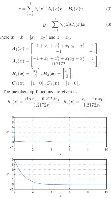
˙ x= 2 i=1 hi(z){Ai(x)ˆx+Bi(x)u} (37) y= 2 i=1 hi(z)Ci(x)ˆx (38) wherex= ˆx=x1 x2andz=x1, A1(x) = −1 +x1+x21+x1x2−x22 1 −1 −1 , A2(x) = −1 +x1+x21+x1x2−x22 1 0.2172 −1 , B1(x) = x1 0 ,B2(x) = x1 0 , C1(x) =1 0,C2(x) =1 0.
The membership functions are given as
h1(z) =sinx11+ 0.2172x1 .2172x1 , h2(z) = x1−sinx1 1.2172x1 . 0 2 4 6 8 10 -2 0 2 4 6 8 10 t x1 0 2 4 6 8 10 -2 0 2 4 6 8 10 t x2
Fig. 1. Guaranteed cost control result.
The SOS design condition in Theorem 1 is feasible when the orders of bothX(˜x)andMi(x)are not zero. Conversely, when the orders of bothX(˜x) andMi(x) are zero, that is, when bothX(˜x)andMi(x)are constant matrices instead of polynomial matrices inx, the design condition in Theorem 1 reduces to the existing LMI design condition. In other words, whenX(˜x)andMi(x)are constant matrices, the polynomial fuzzy controller reduces to the Takagi-Sugeno fuzzy controller. Only in this case, the SOS design condition in Theorem 1 is infeasible. This means that the polynomial fuzzy controller stabilizes globally and asymptotically the polynomial fuzzy system (37) although it may be difficult to stabilize globally and asymptotically the nonlinear system via Takagi-Sugeno fuzzy controllers.
The guaranteed cost controllers for Q = I, R = 1 and x(0) = 10 10T gives J = 183.3 when the orders of X(˜x) and Mi(x) are 0 and 1. The stable polynomial fuzzy controller designed in [11] gives J = 297.7. Thus,
the performance index value of the guaranteed cost control is better than that of the stable control. In addition, if the orders of X(˜x) and Mi(x) are increased, the performance index value can be improved. For example, the guaranteed cost control gives J = 144.0 when the order ofMi(x) are 2. Furthermore, the guaranteed cost control givesJ = 131.0
when the orders ofX(˜x)andMi(x)are 2 and 3, respectively. A main difference between the Takagi-Sugeno fuzzy model and the polynomial fuzzy model is that (37) can have x1
and x2 in the Ai and Bi matrices, i.e., that Ai and Bi are permitted to be polynomial matrices in x. Furthermore, our approach deals with a more general Lyapunov function (polynomial Lyapunov function). Thus, our approach provides more relaxed design results than the existing LMI approach. In addition, the polynomial fuzzy model (37) is an exact global model for the nonlinear system though the Takagi-Sugeno fuzzy model (33) is an (exact) semi-global model for the nonlinear system.
B. Micro Helicopter Control
A co-axial counter rotating helicopter dynamics can be written as ˙ u(t) =− a Izψ(t)v(t) + 1 mUX(t), (39) ˙ v(t) =a Izψ(t)u(t) + 1 mUY(t), (40) ˙ w(t) =1 mUZ(t), (41)
under some assumptions [17], wherea = 1.5, m= 0.2 and
Iz = 0.2857. u, v and w denote velocities of x, y and z axis directions, respectively.ψis angle around zaxis.UX(t),
UY(t)andUZ(t)denote control input variables.
Based on the concept of sector nonlinearity [1], the non-linear system can be exactly represented by a Takagi-Sugeno fuzzy model for ψ(t) ∈ [−π π]. The Takagi-Sugeno fuzzy
model is obtained as ˙ x(t) = 2 i=1 hi(z(t)){Aix(t) +Biu(t)}, (42) y(t) = 2 i=1 hi(z(t))Cix(t), (43) wherez(t) =ψ(t)and x(t) = [u(t)v(t)w(t)ex(t)ey(t)ez(t)]T, u(t) = [UX(t)UY(t) UZ(t)]T.
The elements ex(t), ey(t) and ez(t) are defined as ex(t) =
x(t)−xref,ey(t) =y(t)−yref,ez(t) =z(t)−zref, where
xref, yref and zref are constant target positions. Ai, Bi andCi matrices and the membership functions are given as
follows. A1= ⎡ ⎢ ⎢ ⎢ ⎢ ⎢ ⎢ ⎣ 0 −aπ IZ 0 0 0 0 aπ IZ 0 0 0 0 0 0 0 0 0 0 0 1 0 0 0 0 0 0 1 0 0 0 0 0 0 1 0 0 0 ⎤ ⎥ ⎥ ⎥ ⎥ ⎥ ⎥ ⎦ , A2= ⎡ ⎢ ⎢ ⎢ ⎢ ⎢ ⎢ ⎣ 0 aπ IZ 0 0 0 0 −aπ IZ 0 0 0 0 0 0 0 0 0 0 0 1 0 0 0 0 0 0 1 0 0 0 0 0 0 1 0 0 0 ⎤ ⎥ ⎥ ⎥ ⎥ ⎥ ⎥ ⎦ , B1=B2= ⎡ ⎢ ⎢ ⎢ ⎢ ⎢ ⎢ ⎣ 1 m 0 0 0 1 m 0 0 0 1 m 0 0 0 0 0 0 0 0 0 ⎤ ⎥ ⎥ ⎥ ⎥ ⎥ ⎥ ⎦ , C1=C2= ⎡ ⎣ 0 0 0 1 0 00 0 0 0 1 0 0 0 0 0 0 1 ⎤ ⎦, h1(ψ(t)) = ψ(t2) +π π , h2(ψ(t)) = π−ψ(t) 2π .
Note that the Takagi-Sugeno fuzzy model exactly represents the dynamics (39) - (41) for the rangeψ(t)∈[−π π].
Consider the performance index (8) again. We can find feedback gains that minimizes the upper bound of (8) by solving the following LMIs [1]. From the solutions X and Mi, the feedback gains can be obtained as Fi =MiX−1. Then, the controller satisfiesJ <xT(0)Xx(0)< λ.
minimize X,Mi, λ subject to X>0, λ xT(0) x(0) X >0, (44) ˆ Uii<0 (45) ˆ Vij<0 i < j, (46) where ˆ Uii = ⎡ ⎣ Hii XC T i −MiT CiX −Q−1 0 −Mi 0 −R−1 ⎤ ⎦, ˆ Vij = ⎡ ⎢ ⎢ ⎢ ⎢ ⎣ Hij+Hji XCiT −MjT XCjT −MiT CiX −Q−1 0 0 0 −Mj 0 −R−1 0 0 CjX 0 0 −Q−1 0 −Mi 0 0 0 −R−1 ⎤ ⎥ ⎥ ⎥ ⎥ ⎦, Hij =XATi +AiX−BiMj−MTjBTi . The above LMI condition is feasible for this fuzzy model.
On the other hand, the SOS design condition in Theorem 1 is also feasible when the orders ofX(˜x)andMi(x)are zero and two, respectively. We compare the LMI-based guaranteed cost controller (designed by solving the (44) - (46)) with the controller (designed by the SOS condition in Theorem 1), that is, with the SOS-based guaranteed cost controller. Table I shows comparison results of performance function values
J for the LMI controllers and the SOS controllers, where the initial positions are u(0) = 0, v(0) = 0, w(0) = 0 ex(0) = −0.6, ey(0) = −0.4 and ez(0) = −1. In Table I, Cases I, II and III denote three cases of selecting the weighting matrices(Q,R) = (I,0.1I),(Q,R) = (I,I), and (Q,R) = (I,10I), respectively.
TABLE I
COMPARISON OF PERFORMANCE FUNCTION VALUESJ
Case I Case II Case III LMI controller 0.67286 1.5522 3.8873 SOS controller 0.57539 1.0388 2.3350 Reduction rate of J[%] 14.4859 33.0756 39.9326 It is found from Table I that the performance index values of the SOS based guaranteed cost control (Theorem 1) are better than those of the LMI based guaranteed cost control ((44) -(46)) in all the cases.
IV. CONCLUSIONS
This paper has presented guaranteed cost control of poly-nomial fuzzy systems via a sum of squares (SOS) approach. First, we have presented a polynomial fuzzy model and con-troller that are more general representation of the well-known Takagi-Sugeno (T-S) fuzzy model and controller, respectively. Secondly, we have derived a guaranteed cost control design condition based on polynomial Lyapunov functions. Hence, the design approach discussed in this paper is more general than the existing LMI approaches (to T-S fuzzy control system designs) based on quadratic Lyapunov functions. The design condition realizes guaranteed cost control by minimizing the upper bound of a given performance function. In addition, the design condition in the proposed approach can be represented in terms of SOS and is numerically (partially symbolically) solved via the recent developed SOSTOOLS. To illustrate the validity of the design approach, two design examples have been provided. Both the examples have shown that our approach provides more extensive design results for the existing LMI approach.
Our future works are to apply this approach to a real micro helicopter and to extend this approach to a variety of control techniques.
ACKNOWLEDGMENT
The authors would like to thank Mr. K. Yamauchi and Mr. T. Komatu, UEC, Japan, for their contribution to this research.
REFERENCES
[1] K. Tanaka and H. O. Wang: Fuzzy Control Systems Design and Analysis: A Linear Matrix Inequality Approach, JOHN WILEY & SONS, INC, 2001.
[2] H.-N. Wu and H.-X. Li, “Finite-Dimensional Constrained Fuzzy Control for a Class of Nonlinear Distributed Process Systems”, IEEE Transactions on Systems, Man and Cybernetics Part B, Vo1. 37, No. 5, pp.1422-1430, Octber, 2007.
[3] W.-W. Lin, W.-J. Wang and S.-H. Yang, “A Novel Stabilization Criterion for Large-Scale T-S Fuzzy Systems”, IEEE Transactions on Systems, Man and Cybernetics Part B, Vo1. 37, No. 4, pp.1074-1079, August, 2007. [4] P. Baranyi, “TP model transformation as a way to LMI based controller
design”, IEEE Transaction on Industrial Electronics, vol. 51, no. 2, pp.387-400, April 2004.
[5] K. Tanaka, et al., “Switching Control of an R/C Hovercraft: Stabilization and Smooth Switching,”, IEEE Transactions on Systems, Man and Cybernetics, Part B, Vol.31, No.6, pp.853-863, Dec. 2001.
[6] C.-H. Sun and W.-J. Wang, “An improved stability criterion for T-S fuzzy discrete systems via vertex expression”, IEEE Transactions on Systems, Man and Cybernetics Part B, Vo1. 36, No. 3, pp.672-678, June, 2006. [7] H. O. Wang, J. Li, D. Niemann and K. Tanaka, “T-S fuzzy Model with
Linear Rule Consequence and PDC Controller: A Universal Framework for Nonlinear Control Systems”, 9th IEEE International Conference on Fuzzy Systems, San Antonio, May, 2000, pp.549-554.
[8] D. Tikk, P.Baranyi, R. J. Patton, “Approximation Properties of TP Model Forms and its Consequences to TPDC Design Framework”, Asian Journal of Control, Vol. 9, No. 3, pp. 221-231, Sept. 2007.
[9] G. Feng, “A Survey on Analysis and Design of Model-Based Fuzzy Control Systems”, IEEE Trans. on Fuzzy Systems, Vol.14, no.5, pp.676-697, Oct. 2006.
[10] K. Tanaka, H. Yoshida, H. Ohtake and H. O. Wang “A Sum of Squares Approach to Stability Analysis of Polynomial Fuzzy Systems”, 2007 American Control Conference, New York, July, 2007, pp.4071-4076. [11] K. Tanaka, H. Yoshida, H. Ohtake and H. O. Wang, “ Stabilization of
Polynomial Fuzzy Systems via a Sum of Squares Approach”, 2007 IEEE International Sympoisum on Intelligent Control, pp.160-165, Singapore, October 2007.
[12] S. Prajna, A. Papachristodoulou, P. Seiler and P. A. Parrilo: SOS-TOOLS:Sum of Squares Optimization Toolbox for MATLAB, Version 2.00, 2004.
[13] T. Takagi and M. Sugeno, “Fuzzy Identification of Systems and Its Applications to Modeling and Control”, IEEE Trans. on SMC 15, no. 1, pp.116-132, 1985.
[14] J. F. Sturm: “Using SeDUMi 1.02, a MATLAB toolbox for optimization over symmetric cones”, Optimization Methods and Software, vol. 11 & 12, pp.625-653, August 1999.
[15] K. C. Toh, R. H. Tutuncu and M. J. Todd, “On the impliment of SDPT3 (version 3.1) -a MATLAB software package for semidefinite-quadratic-linear programming”, 2004 IEEE International Conference on Computer Aided Control System Designs, pp.290-296, Sept. 2004.
[16] S. Prajna, A. Papachristodoulou and F. Wu: “Nonlinear Control Syn-thesis by Sum of Squares Optimization: A Lyapunov-based Approach”, Proceedings of the Asian Control Conference (ASCC), Melbourne, Aus-tralia, Feb. 2004, pp.157-165.
[17] K. Tanaka, T. Komatsu, H. Ohtake and H. O. Wang, “Micro Helicopter Control: LMI approach vs SOS approach”, 2008 IEEE International Conference on Fuzzy Systems, pp.347-353, Hong Kong, June 2008.