Influence Function and Efficiency of the Minimum Covariance Determinant Scatter Matrix Estimator

Influence Function and Efficiency of the Minimum

Covariance Determinant Scatter Matrix Estimator

Christophe Croux

Universite Libre de Bruxelles,Brussels,Belgium

E-mail: ccrouxulb.ac.be

and

Gentiane Haesbroeck University of Liege,Liege,Belgium

E-mail: G.Haesbroeckulg.ac.be Received June 2, 1998

The minimum covariance determinant (MCD) scatter estimator is a highly robust estimator for the dispersion matrix of a multivariate, elliptically symmetric distribution. It is relatively fast to compute and intuitively appealing. In this note we derive its influence function and compute the asymptotic variances of its elements. A comparison with the one step reweighted MCD and with S-estimators is made. Also finite-sample results are reported. 1999 Academic Press

AMS 1991 subject classifications: 62F35, 62G35.

Key words and phrases: influence function; minimum covariance determinant estimator; robust estimation; scatter matrix.

1. INTRODUCTION

The classical average and covariance matrix are key ingredients in almost all multivariate statistical methods. However, they are extremely sensitive to outliers. It is therefore important to consider robust alternatives for these estimators, which can be used to obtain robust procedures in principal component analysis, factor analysis, etc. Among the robust alter-natives to the classical estimators, the minimum volume ellipsoid (MVE) introduced by Rousseeuw (1985) is probably the most widely known and used (e.g., by He and Wang, 1996). It consists of taking as location estimator the center of the smallest regular ellipsoid containing half the points of the data set. The scatter estimator is then defined by the shape

161

0047-259X9930.00

Copyright1999 by Academic Press All rights of reproduction in any form reserved.

matrix of that ellipsoid. However, it was shown that the MVE estimator is not -n consistent (Davies, 1992a), making it less attractive for efficiency reasons. A robust estimator which has the normal rate of convergence is the minimum covariance determinant (MCD) estimator of Rousseeuw (1985). The location and scatter estimates are given by the average and covariance matrix computed on that half of the data which attain the smallest determinant of their covariance matrix. Until quite recently, the major drawback of the MCD estimator was its computation time. Rousseeuw and Van Driessen (1999) however, proposed a new algorithm to compute MCD, which turns out to be extremely fast, even in high dimensions. Theoretical properties of the MCD estimator have been investigated in Butler (1982) and Butler, Davies, and Jhun (1993), but the asymptotic distribution of the scatter part of the MCD remained unknown. In the particular case of one dimension the influence function of the MCD scale was computed by (Croux and Rousseeuw, 1992).

The main focus of this paper is to derive the influence function of the MCD scatter matrix in arbitrary dimensions. Second, the influence function is used to calculate asymptotic variances and efficiencies for the MCD and its reweighted version. Third, the finite-sample behavior is investigated by means of a simulation study. Furthermore, a thorough comparison with multivariate S-estimators is included.

The outline of the paper is as follows. Section 2 defines the MCD-func-tional and gives its influence function while in Section 3 asymptotic varian-ces are computed. Section 4 uses results of Lopuhaa (1997) to show that one step reweighted covariances, starting from MCD based weights, com-bine the breakdown properties of the MCD estimator while achieving a better asymptotic efficiency. However, this reweighting does not yield an estimator as efficient as the S-estimator of scatter. Finite-sample results based on simulations are reported in Section 5 while Section 6 contains some conclusions.

2. INFLUENCE FUNCTION

For a finite sample of observations [x1, ...,xn] inRpthe MCD is

deter-mined by selecting that subset [x_i1, ...,x_ih] of sizeh, with 1hn, which minimizes the generalized variance (which is the determinant of the covariance matrix computed from the subset) among all possible subsets of size h. The location estimator is then defined as

+^n= 1 h : h j=1 xij

and the estimator of scatter by 7 n=cp 1 h : h j=1 (xij&+^n)(xij&+^n) t_,

where cp is a consistency factor. The choice h=[(n+p+1)2] is

com-monly preferred since it yields the highest possible breakdown point

(Lopuhaa and Rousseeuw 1991). Note that hrn

2 at least if the number of observations is much higher than the dimension. The breakdown point of a multivariate scale estimator is defined as the smallest fraction of observa-tions that you need to replace to arbitrary position before the estimated scatter explodes (its biggest eigenvalue tends to infinity) or implodes (its smallest eigenvalue tends to zero). Another default value ishr0.75n,

yield-ing a better compromise between efficiencystability and high breakdown.

To derive the influence function of an estimator, we need a proper defini-tion for its funcdefini-tional form. In Butler, Davies, and Jhun (1993; BDJ from now on) a definition appropriate for continuous distributions is given,

which we will generalize afterwards to arbitrary distributions G. This is

necessary since we will apply the MCD to point contaminated distribu-tions.

Denote by 0<:<1 the mass of the data not determining the MCD,

which will result in an estimator with (asymptotic) breakdown point min(:, 1&:). Define

DG(:)=[A|ARpmeasurable and bounded withPG(A)=1&:], (2.1)

and for every A#DG(:), the average and covariance matrix computed over

this set will be denoted by

TA(G)= _Ay dG(y) 1&: (2.2) and 7A(G)= A(y&TA(G))(y&TA(G))tdG(y) 1&: . (2.3)

The setA is called an MCD-solution if

det(7A(G))det(7A(G)), (2.4)

for every other A#DG(:). The MCD estimators at the theoretical

distribu-tion are then defined by

for an MCD solutionA. The constantc:can be chosen in such a way that

consistency will be obtained at the specified model.

A problem may arise with the above definition when the distribution G

is not continuous, in which caseDG(:) may be empty. Therefore define

D G(:)=[(A,x) |ARpmeasurable and bounded,x#Rp"A

and _0$PG([x]) :PG(A)+$=1&:],

which is never empty. Furthermore, for every (A,x) #D G(:) define (with

$=1&:&P_G(A)) T₍A,x)(G)= Ay dG(y)+$x 1&: , (2.6) and 7(A,x)(G)=(1&:)&1

{

|

A (y&T(A,x)(G))(y&T(A,x)(G))tdG(y) +$(x&T(A,x)(G))(x&T(A,x)(G))t

=

. (2.7) (Since Ais bounded all the above quantities are well defined). We say that (A,x) #D G(:) is an MCD solution if

det(7(A,x)(G))det(7(A,x~)(G)), (2.8)

for every (A,x~) #D G(:). The MCD estimators at the population level are

then given by

T(G)=T(A,x)(G) and 7(G)=c:7(A,x)(G), (2.9)

for an MCD solution (A,x). Thus, the MCD solution determines a region

B=A_[x], with PG(A)1&:PG(B). By giving a lower mass to the

atom x, we are in a certain way interpolating between the two setsAandB. For ease of notation, we will write TA(G) and 7A(G) instead ofT(A,x)(G) and 7(A,x)(G) wheneverPG(A)=1&: for a couple (A,x) #D G(:).

In this paper we will focus on the problem of estimating the parameters

+ and 7of the distribution F+,7with density

f+,7(x)=

g((x&+)t₇&1_(x&+))

-det(7) (2.10)

The function g is assumed to be known and to have a strictly negative derivativeg$, so thatF+,7belongs to a parametric class of elliptically

sym-metric, unimodal distributions. It is shown in Section 2 of BDJ that for this distribution the MCD-problem has a unique solution given by the ellipsoid

A(F+,7)=[z#Rp| (z&+)t7&1(z&+)q:], (2.11)

where G(t)=PF0,I(Z

t_{Zt) andq}

:=G&1(1&:), with corresponding

MCD-functionals T(F+,7)=+ 7(F+,7)=

\

c_: 1&:

|

zt_zq : z2 1 dF0,I(z)

+

7.

To obtain Fisher-consistency at this model, it suffices to set

c:= 1&: zt_zq:z2₁dF_0,I(z) =(1&:)

{

? p2 1(p2+1)

|

-q: 0 rp+1_g(r2_)dr

=

&1. Table I gives several values of the constants c: andq: for different values

ofp and : at the normal model.

Since the MCD is affine equivariant we will only derive the influence function at the model distribution F=F0,Ip. Consider the contaminated

distribution

F=,x=(1&=)F+=2x,

where2x is a Dirac measure putting all its mass at x#Rp. The influence

function measures the sensitivity of the MCD-functional to small amounts of contamination in the distribution:

IF(x,7,F)=lim

=a0

7(F=,x)&7(F)

= .

More about the use and interpretation of influence functions can be found

in Hampel et al. (1986). The derivation of the influence function for the

MCD relies on the following proposition, which says that the MCD solu-tion at the contaminated distribusolu-tion F=,x is still determined by an

ellip-soid. (This can even be shown to be true for any distributionG, and was

TABLE I

Particular Values ofc:andq:at the Normal Model

: p=2 p=3 p=5 p=10 p=30

0.25 c: 1.859 1.609 1.412 1.256 1.130

q: 2.773 4.108 6.626 12.549 37.799

0.5 c: 3.259 2.457 1.912 1.531 1.257

q: 1.386 2.366 4.351 9.342 29.336

Proposition 1. Take 0<=<min(:, 1&:), x#Rp and consider the

con-taminated distribution F=,x. For any MCD-solution (A, y) #D F=,x(:), there

exists an open ellipsoid Esuch that

E#DF=,x(:), TE(F=,x)=T(A,y)(F=,x), and 7E(F=,x)=7(A,y)(F=,x)

or, in the special case that x lies at the border ofE, (E,x) #D _F=,x(:),

T_(E,x)(F=,x)=T(A,y)(F=,x), and 7(E,x)(F=,x)=7(A,y)(F=,x).

The next theorem gives the influence function of the scatter matrix part of the MCD functional. To facilitate the interpretation, we give separate expressions for the diagonal and off-diagonal elements. All proofs are kept for the Appendix.

Theorem 1. With the notations from above, we have that

IF(x,7ii,F)= 1 b₁

{

c_: 1&:x 2 i I(&x& 2_q :)+ b₂ b₁&pb₂ c_:

1&:&x&

2_I(&x&2_q :) + b1 b₁&pb₂

_

c_: 1&: q_:

p (1&:&I(&x&

2_q :))&1

&=

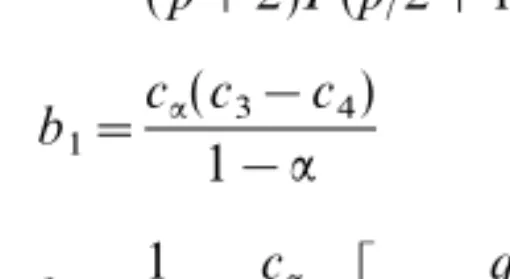
(2.12) IF(x,7ij,F)= xixj &2c3 I(&x&2_q :) ifi{j, (2.13)

where the constants b1,b2,c2,c3, and c4 are determined by the relations

c2= ?p2 1(p2+1)

|

-q: 0 rp+1_g$(r2_)dr c3=

{

?p2 (p+2)1(p2+1)

|

-q: 0 rp+3_g$(r2_{)dr if p2} 0 otherwise

c4= 3? p2 (p+2)1(p2+1)

|

-q: 0 rp+3_g$(r2 )dr b1=c:(c3&c4) 1&: b2=1 2+ c: 1&:

_

c3& q: p

\

c2+ 1&: 2

+&

.

It follows immediately that the MCD scale estimator has a bounded influence function, which is redescending to zero for the off-diagonal elements, but not for the on-diagonal elements. In Fig. 1 the influence func-tionsIF(x,711,F) andIF(x,712,F) are pictured for p=2 and :=0.25 at the normal model. The functions are smooth, except for a jump at the circle with radius-q:. If we denote %the angle of xwith the first axis, then the discontinuity in IF(x,711,F) is upwards for %<?4 and downwards for

%>?4. The maximal value is attained at (-q:, 0). The off-diagonal influence function is maximal at (-q:2,-q:2).

Remark 1. For p>1 one can see that c4=3c3 and the obtained influence function can be rewritten in the more compact form

IF(x,7,F)=&1 2c3

xxt_I(&x&2_q

:)+w(&x&)Ip,

wherewis a certain real valued function.

FIG. 1. Influence function of the MCD scale estimator at the normal model, withp=2, and :=0.25, (a) for the first diagonal element of the scatter matrix (b) for an off-diagonal element of the scatter matrix.

Remark 2. The classical estimator of a scatter matrix is the covariance matrix C(G), defined at the population level by

C(G)=c₀

_|

Rp(

x&+(G))(x&+(G))t_{dG(x), (2.14)}

where +(G)=_RpxdG(x) and the consistency factor c₀ equals E_F(X2_i)&1

whereXi is a component of the vector X. It appears as a limit case of the

MCD for:, the mass of the data ``discarded'' by the MCD, tending to zero.

Note that C is only well defined for distributions with a second moment,

whereas the MCD functionals are properly defined for arbitrary distribu-tions. It is not so difficult to check that

lim

:a0

IF(x,7,F)=c₀xxt_{&I=IF(x,C,F).}

Remark 3. In the case p=1, (2.12) can be rewritten as

IF(x,7,F)=

{

|

-q:

&-q:

t2_dF(t)

=

&1[I( |x| -q:)(x2&q:)+(1&:)q:]&1,

with -q_:=F&1_{(1&:2). The parameter S=-7 measures here the} dis-persion of the univariate distributionF. This above expression corresponds with the results of Croux and Rousseeuw (1992).

Remark 4. The computation of the influence function of the location part of MCD is relatively simple, and the result is implicitly contained in BDJ:

IF(x,T,F)=

\

&2 1&:

|

zt_zq:

zzt_g$(zt_z)dz

+

&11&x:I(&x&

2_q

:).

Observe that IF(x,T,F) becomes zero when x is outside the ball of radius -q_:, illustrating that MCD-location ``rejects'' huge outliers. This is in contrast with MCD-scatter, where these outliers still have a (bounded) influence on the diagonal elements of the scatter matrix.

Attention in this paper is restrained to the scale case, but also highly robust affine equivariant estimation of location is of interest (e.g. for application in MANOVA models). It is however well known (Rousseeuw and Leroy, 1987, p. 271) that with an orthogonally equivariant location estimator T0 and an

affineequivariant scatter matrix estimator 70, an affine equivariant location estimatorT1is easily obtained by setting

T₁(x₁, ...,x_n)=712

0 T0(7&10 2x1, ...,7&10 2xn).

Lopuhaa (1992) proved thatT1inherits the robustness properties of the initial

estimators which have high breakdown point, good efficiency properties and which are very fast to compute have been proposed in the literature (e.g., Hossjer and Croux, 1994).

Remark 5. Strictly speaking, Theorem 1 only gives an almost sure expres-sion for the influence function. In case that&x&2_=q

:, a zero probability event,

one has IF(x,7,F)=c:xxt&I. This follows quite immediately from the

special case of Proposition 1.

3. ASYMPTOTIC VARIANCES

It follows from BDJ (by taking g(x)=xxt_{I(x#E&C) in the proof of}

Theorem 4, page 1397) that the MCD scatter matrix is asymptotically normal, but no expression for the asymptotic variance has been derived there. In this section we will compute asymptotic variances by means of

ASV(7ij,F)=

|

RpIF

2_(x,7

ij,F)dF(x) (3.1)

for 1i, jn. The above expression certainly holds if the MCD-functional is Frechet differentiable but a formal verification is still open. To our knowledge, a proof of Frechet differentiability has not been given yet in the literature. The normal location-scale model (2.10) with

g8(t)=

1

(2?)p2exp

\

&

t

2

+

is without any doubt the most important case. We will denoteF=8the mul-tivariate standard normal distribution. Explicit expressions for the asymptotic variances can be worked out:

ASV(7ii,8)=[b1(b1&pb2)(1&:)]&2

[(1&:)b2

1(:((c:q:p)&1)2&1)&2c3c2:(3(b1&pb2)2 +(p+2)b2(2b1&pb2))]

ASV(7ij,8)= &

1 2c3

if i{j.

Please note that the above expressions vary both with the dimensionp and

with the trimming proportion :. The limit case :=0 gives the asymptotic

variances of the usual covariance matrix:

These asymptotic variances are used to compute the asymptotic efficiencies of the estimators at a model distributionF, which are defined by the ratios

Eff(7ij,F)=

1

ASV(7_ij,F)J(7_ij,F) \1i, jp, (3.2) where the inverse of the Fisher Information J(7ij,F) is the Cramer-Rao

lower bound. It is well known that the classical covariance matrix attains the lower bound at normal models.

Figure 2 illustrates how the asymptotic efficiencies Eff(7ij,8) vary with :

and p under the normal model. First of all, note that efficiency decreases as the breakdown point increases, showing a conflict between efficiency and high breakdown. Choosing the highest possible breakdown point (:=0.5) results in a severe loss of efficiency. The suggestion to take :=0.25 as a compromise between efficiency and robustness finds its motivation here: the corresponding estimator can still cope with realistic amounts of contamination in the data, but is much more precise (when no outliers are present) than the usual choice :=0.5. One should not forget that the bias of the MCD with:=0.25 remains

bounded for percentages of contamination smaller than 250 but can still

become unpractically large. In these cases, the maximal breakdown point

MCD may become an alternative. Optimally, a data-driven choice of:should

be undertaken, but this possibility has not been explored further.

Figure 2 also reveals that the efficiencies of MCD are increasing with the dimension. Even more, one can formally prove that

lim

pÄEff(

7_ij,8)=1&: \1i, jp. (3.3)

Result (3.3) can be understood intuitively: every observationX_i=(X_i1, ...,X_ip)t

following the reference distribution8lies at a squared distanceX2

i1+ } } }X 2

iprp

FIG. 2. Asymptotic efficiency of respectively (a) a diagonal element (b) an off-diagonal element of the MCD scatter matrix estimator at the normal model for several values ofpand :varying in (0, 0.5).

from the origin, when p is large. (Here we used the strong law of large numbers and independency of the different components ofXi.) This implies

that all observations are ``equally likely'' to constitute the subset of size

n(1&:) whose covariance matrix will yield the MCD-scatter estimator. We

conclude that, at the reference distribution8and forp huge, the MCD is

like a usual covariance matrix but computed from a random subsample of size n(1&:) instead of size n, which explains (3.3). The convergence in

(3.3) is however rather slow, as is shown by the table below for:=0.25:

p 100 103 ₁₀4 ₁₀7

Eff(7ii,8) 0.6559 0.7210 0.7415 0.7497 0.75

Eff(7ij,8) 0.6542 0.7209 0.7411 0.7497 0.75

Another class of multivariate elliptically symmetric distributions which is regularly used (e.g. in econometrics), is generated by setting in (2.10)

g_F&(t)=1((p+&)2)

1(&2)(?&)p2

1

(1+(tv))(p+&)2.

The corresponding model distribution is a multivariate Student with &

degrees of freedom. Consistency factors and influence functions can be

easily computed, using symbolic computation software. Moreover,

asymptotic variances have been computed by (3.1) for the reference dis-tributionF&, using numerical integration and a lot of computation time in

order to obtain accurate results. The classical covariance estimator (2.12) needs now to be premultiplied with c0=(&&2)&, and has asymptotic variances ASV(Cii,F&)=(2&&2)(&&4) and ASV(Cij,F&)=(&&2)(&&4)

for &>4 and i{j. The Fisher Informations at F& are equal to

J(7ii,F&)=(p+&&1)(2(p+&+2)) and J(7ij,F&)=(p+&)(p+&+2)

for i{j.

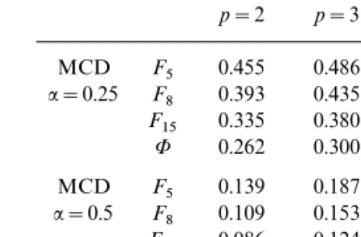
Tables II and III list the asymptotic efficiencies of the elements of the

MCD estimator at some Student distributions F_& with & degrees of

freedom, for several values of p and for :=0.25 and 0.5. Corresponding

values for the normal distribution (which is the limit case for &Ä_{) are} also reported. One sees that at these heavier tailed distributions it remains true that the efficiency gain taking:=0.25 instead of the usual :=0.5 is considerable. Moreover, at the Student distribution with 5 degrees of

freedom, the MCD (with:=0.25) is even more efficient than the classical

TABLE II

Asymptotic Efficiencies of a Diagonal Element of the MCD Scatter Matrix with:=0.25 and 0.5 and of the Covariance MatrixCat

Some Student Distributions for Several Values ofp

p=2 p=3 p=5 p=10 p=30 MCD F5 0.455 0.486 0.528 0.560 0.580 :=0.25 F8 0.393 0.435 0.496 0.558 0.620 F15 0.335 0.380 0.455 0.548 0.617 8 0.262 0.300 0.366 0.459 0.577 MCD F5 0.139 0.187 0.253 0.325 0.393 :=0.5 F8 0.109 0.153 0.284 0.307 0.395 F15 0.086 0.124 0.184 0.275 0.380 8 0.062 0.089 0.134 0.205 0.310 C F5 0.375 0.357 0.333 0.304 0.272 F8 0.762 0.743 0.714 0.672 0.618 F15 0.935 0.926 0.912 0.886 0.841 8 1.000 1.000 1.000 1.000 1.000

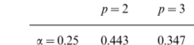
Remark. Table IV reports the asymptotic efficiencies (only for the diagonal elements) of the MCD estimator at the Cauchy distribution (which is a Student distribution with 1 degree of freedom). The results are less clearcut here: the best choice in high dimensions is:=0.5. Notice that the efficiencies in Table IV decrease with the dimension.

TABLE III

Asymptotic Efficiencies of an Off-diagonal Element of the MCD Scatter Matrix with:=0.25 and 0.5 and of the Covariance MatrixC

at Some Student Distributions for Several Values ofp

p=2 p=3 p=5 p=10 p=30 MCD F5 0.284 0.375 0.474 0.564 0.623 :=0.25 F8 0.241 0.332 0.440 0.551 0.639 F15 0.206 0.291 0.398 0.521 0.639 8 0.163 0.233 0.324 0.438 0.570 MCD F5 0.069 0.124 0.206 0.307 0.403 :=0.5 F8 0.055 0.103 0.178 0.283 0.397 F15 0.045 0.085 0.151 0.252 0.380 8 0.033 0.063 0.113 0.191 0.304 C F5 0.429 0.417 0.400 0.378 0.352 F8 0.800 0.788 0.770 0.741 0.702 F15 0.946 0.940 0.931 0.914 0.884 8 1.000 1.000 1.000 1.000 1.000

TABLE IV

Asymptotic Efficiencies of a Diagonal Element of the MCD Scatter Matrix Estimator at the Cauchy Distribution for

Several Values ofpwith:=0.25 and 0.5

p=2 p=3 p=5 p=10 p=30

:=0.25 0.443 0.347 0.279 0.229 0.198

:=0.5 0.356 0.322 0.294 0.266 0.247

4. RELATED ROBUST ESTIMATORS OF SCATTER

Since the efficiency of high breakdown methods at normal distributions can be quite low, it is often recommended to compute reweighted versions of them, which maintain the breakdown point of the initial estimators while attaining (hopefully) a better efficiency. Quite recently, Lopuhaa (1997) derived asymptotic properties of reweighted multivariate estimators of location and scatter. Denote (T0_,70_{) initial robust estimators of} multi-variate location and scatter. For a sample [x₁, ...,x_n] one step reweighted estimators are computed as

T1₌ n i=1wixi n i=1wi and 71_=c 1 n i=1wi(xi&T1)(xi&T1)t n i=1wi , (4.1)

where the weights are computed from the initial estimators by

wi=w((Xi&T0)t(70)&1(Xi&T0))

with w: [0,[Ä_{Ra suitable weight function.} A simple, but common choice is to take

w(t)=I[0,q$](t) withq$=G

&1_{(1&$), (4.2)}

where G(u)=PF(XtXu). At the p-dimensional normal model we have

q$=/2p, 1&$. The consistency factorc1 is given by

c₁=(1&$)

{

? p2 1((p2)+1)

|

-q$ 0 rp+1_g(r2_)dr

=

&1.

The influence function of 71

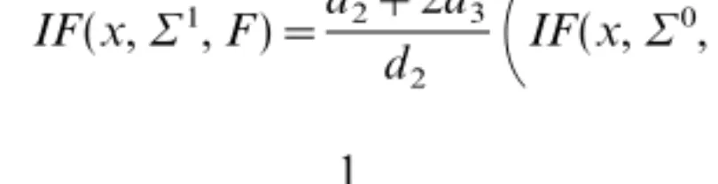
at the model distribution F for the weight

function (4.2) follows from Lopuhaa (1997),

IF(x,71 ,F)=d2+2d3 d2

\

IF(x,70 ,F)+1 2trace(IF(x,7 0 ,F))I

+

+1 d2 I(xt_xq $)xxt&I,

where the constant d2 equals (1&$)c &1

1 and the expression for d3 is the

same as for c3 (given in Theorem 1) but with: replaced by$.

Taking the MCD estimator for (T0_,70_{) and $=0.025 in (4.2) is}

advocated and used by (Rousseeuw and Van Driessen, 1999) and we denote the resulting estimator by MCD1_{. Figure 3 gives the influence}

func-tions for a diagonal and an off-diagonal element of the MCD1

scatter

estimator in the bivariate case for:=0.25. We observe two jumps: one due

to the discontinuity of the weight function and the other due to the discon-tinuity in the influence function of the initial MCD estimator. Note that the

influence of extreme outliers on MCD1

is smaller than on the ordinary MCD.

One could also iterate the process and define MCD2

as a reweighted

estimator using MCD1

as starting estimator in (4.1). The general belief is that reiterating could increase efficiency, but at the cost of a higher bias (Rousseeuw and Croux, 1994).

FIG. 3. Influence function of the one step Reweighted MCD scale estimator at the normal model, withp=2, and:=0.25, (a) for the first diagonal element of the scatter matrix (b) for an off-diagonal element of the scatter matrix.

As a competitor for the MCD estimator, S-estimators will be considered. Recall that the S-functional (t(G),S(G)) is defined as the minimizer of det(S) subject to

|

\(-(x&t)t_S&1

(x&t))dF(x)=b0

among all (t,S), with t#Rp _{and S# PD(p). The function \: [0,[Ä}

[0, +[ should be bounded, increasing and sufficiently smooth. A

standard choice is Tuckey's biweight function:

\_c(y)=min

\

y 2 2& y4 2c2+ y6 6c4, c2 6

+

.

To obtain Fisher consistency at the model distribution F take b0=

EF[\c(&x&)]. In order to attain a breakdown point of :, one needs to

select the constant c as the solution of the equation b0=:\c(). The

reweighted version of an S-estimator which will be considered, S1

, is obtained using the biweight S as initial estimator in (4.1). Asymptotics of S-estimators were derived by Davies (1987) and an expression for the influence function can be found in Lopuhaa (1989). Figure 4 pictures

IF(x, S11,8) andIF(x, S12,8), for the 250breakdown biweight S-estimator. Comparison with Figure 1 reveals that the IF for the S-estimator can be considered as a smoothed version of the MCD's influence function.

Some conclusions about the comparison of the different influence func-tions can now be given. The influence function of the MCD estimator looks like that of the usual covariance matrix at the center of the distribution.

FIG. 4. Influence function for the 250breakdown biweight S-estimator at the normal model, withp=2, and:=0.25, (a) for the first diagonal element of the scatter matrix (b) for an off-diagonal element of the scatter matrix.

However, points further away (which can be considered as outliers) are downweighted by MCD. The same holds for the influence function of

MCD1 _{but there the downweighting happens for points somewhat further}

away from the origin. Moreover, two circles of discontinuity instead of one

appear in the graph of IF(x, MCD1_{,8). The big advantage of the}

S-estimator is that its influence function is very smooth, also downweights outliers and resembles the influence function of the covariance matrix at the center of the distribution. One could conclude that, with respect to influence functions, an S-estimator is to be preferred.

A comparative study of the asymptotic efficiencies of the elements of the

scatter matrix estimators MCD1_{, MCD}2_{, S, and S}1 _{has been done, of}

which the results are reported in Tables V and VI. As before, the two cases

:=250 and 500breakdown point are considered.

TABLE V

Asymptotic Efficiency of a Diagonal Element of the Reweighted MCD and S Scatter Matrices with:=0.25 and 0.5 and of the Covariance MatrixCat

Several Student Distributions.

: p=2 p=3 p=5 p=10 p=30 0.25 8 MCD1 _{0.599 0.680 0.753 0.836 0.901} MCD2 _{0.573 0.656 0.727 0.806 0.872} S 0.899 0.941 0.968 0.990 0.997 S1 _{0.678 0.745 0.793 0.853 0.905} C 1.000 1.000 1.000 1.000 1.000 F5 MCD1 _{0.760 0.743 0.698 0.655 0.577} S 0.899 0.876 0.835 0.765 0.691 C 0.375 0.357 0.333 0.304 0.272 F8 MCD1 _{0.739 0.778 0.778 0.776 0.725} S 0.930 0.942 0.923 0.884 0.819 C 0.762 0.743 0.714 0.672 0.618 F15 MCD1 _{0.695 0.760 0.809 0.843 0.821} S 0.932 0.962 0.980 0.965 0.906 C 0.935 0.926 0.912 0.886 0.841 0.5 8 MCD1 _{0.455 0.595 0.720 0.820 0.896} MCD2 _{0.572 0.651 0.731 0.808 0.877} S 0.502 0.647 0.803 0.920 0.973 S1 _{0.633 0.706 0.782 0.849 0.909} F5 MCD1 _{0.702 0.737 0.709 0.668 0.586} S 0.639 0.718 0.778 0.796 0.783 F8 MCD1 _{0.651 0.749 0.780 0.786 0.730} S 0.603 0.712 0.810 0.859 0.872 F15 MCD1 _{0.579 0.706 0.799 0.844 0.825} S 0.564 0.694 0.828 0.925 0.933

TABLE VI

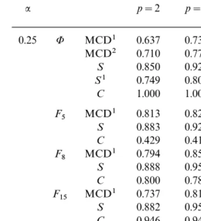
Asymptotic Efficiency of an Off-diagonal Element of the Reweighted MCD and S Scatter Matrices with:=0.25 and 0.5 and of the Covariance Matrix

Cat Several Student Distributions

: p=2 p=3 p=5 p=10 p=30 0.25 8 MCD1 _{0.637 0.736 0.814 0.878 0.928} MCD2 _{0.710 0.773 0.829 0.881 0.929} S 0.850 0.924 0.967 0.988 0.997 S1 _{0.749 0.804 0.849 0.891 0.932} C 1.000 1.000 1.000 1.000 1.000 F5 MCD1 _{0.813 0.822 0.807 0.772 0.709} S 0.883 0.929 0.936 0.905 0.851 C 0.429 0.417 0.400 0.378 0.352 F8 MCD1 _{0.794 0.856 0.873 0.866 0.809} S 0.888 0.951 0.975 0.958 0.911 C 0.800 0.788 0.770 0.741 0.702 F15 MCD1 _{0.737 0.819 0.884 0.912 0.892} S 0.882 0.954 0.990 0.991 0.961 C 0.946 0.940 0.931 0.914 0.884 0.5 8 MCD1 _{0.401 0.618 0.783 0.873 0.934} MCD2 _{0.684 0.765 0.836 0.884 0.934} S 0.377 0.579 0.778 0.915 0.979 S1 _{0.682 0.765 0.842 0.890 0.934} F5 MCD1 _{0.683 0.794 0.811 0.779 0.712} S 0.466 0.637 0.785 0.879 0.910 F8 MCD1 _{0.619 0.804 0.871 0.873 0.812} S 0.440 0.626 0.798 0.913 0.956 F15 MCD1 _{0.531 0.742 0.871 0.915 0.894} S 0.414 0.611 0.800 0.933 0.985

First of all, note that there is no real efficiency gain using MCD2_instead

of MCD1_{, at least for :=0.25. In the 500 breakdown case, where the}

efficiency of the initial estimator MCD is very low (cf. Fig. 2), two times reweighting may be an option. A comparison with Tables II and III shows that a considerable asymptotic efficiency gain is obtained by reweighting the MCD-estimator. Also at the heavier tailed Student distributions,

MCD1 _{is more precise than ordinary MCD and even achieves a better}

efficiency than the classical estimator for small values of&. As a preliminary

conclusion, one can say that the one step reweighted 250 breakdown

MCD seems to be the best out of the class of MCD-based estimators.

On the other hand, the 250breakdown S-estimator outperforms all the

others in the normal case (except the classical estimator) and under the Student distributions. Using the reweighted S-estimator for efficiency

reasons has not much sense, unless for:=500andpsmall. The ordinary S-estimator combines a high efficiency with a high breakdown point, yield-ing a very appealyield-ing estimator. Rocke (1996) noticed that the efficiency of

S-estimators tends to 1000 when the dimension tends to infinity, but

argued that S-estimators are in fact not so robust since their asymptotic

rejection probability is extremely small in high dimensions. One may not forget that a positive breakdown point is not a guarantee for robustness, since the corresponding bias may become extremely large, but still remain bounded.

5. FINITE SAMPLE EFFICIENCIES

The results given in the preceeding sections are of an asymptotic nature. In this section, finite-sample efficiencies for the MCD, S and their reweighted versions are obtained by means of a simulation study. Both estimators are defined as minimizers of a certain criterion under an addi-tional constraint, implying that it is not so obvious to compute them in practice. Fortunately, algorithms were proposed which give approxima-tions to the actual value of the estimator. For computing the MCD the FAST-MCD algorithm of Rousseeuw and Van Driessen (1999) was used, while S-estimators are based on the SURREAL algorithm of Ruppert (1992). Both algorithms start from an initial mean and covariance matrix

obtained from a (p+1) subset of observations, which is iterated towards

better approximations using Newton-steps (for S) or the so-called C-steps

which are used in the FAST-MCD algorithm. This choice for the starting values guarantees that the computed version of the estimator shares the robustness properties of the theoretical counterpart. Implementation of the algorithms was done in GAUSS and in both cases 500 different starting values were considered for each computation of the estimator. To illustrate the fastness of the algorithms: at a (50 _ 5) normal data set it took about one second to compute the MCD and half a second for the S-estimator on a Pentium 200Mhz. One may certainly say that computational feasibility is no longer an obstacle for the use of high breakdown methods (at least not

for small p). Furthermore, note that reweighting the estimators comes at

almost no additional computational cost.

For m=5000 samples of sizes n=50 and 200, observations were

generated from a N(0, Ip) with p=2, 3, 5 or 10. Denote 7 kij the element

(i, j) of the estimator obtained from the kth sample, with 1km. The

accuracy of a diagonal element is measured by the standardized variance

StVar(7 ii)=

nvarm(7 ii)

[avem(7 ii)]2

where avem(7 ii) and varm(7 ii) are the average and variance computed from

the sequence of m replicates 7 k

ij. (Use of measure (5.1) is motivated by

Bickel and Lehmann, page 1142, 1976). For an off-diagonal element the mean squared error (MSE) is used to measure the deviation from the true value, MSE(7 ij)= n m : m k=1 (7 k ij&Iij)2, (5.2)

with I_ij of course equal to zero fori{j.

The simulation results are summarized in Tables VII and VIII. Since 2 is the lower bound for (5.1), the reported efficiencies in Table VII equal 2avepStVar(7 ii). Efficiencies for the off-diagonal elements are obtained in

a similar way, now with 1 as lower bound. The standard error of any value

reported in the tables equals approximately 20of the value.

First off all, note that the finite-sample efficiencies of the MCD converge

well to the asymptotic ones which are listed under n= in the tables.

There is some discrepancy for p=10, which enforces the idea that

con-vergence to the asymptotic distribution is slower in higher dimensions.

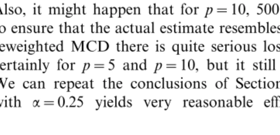
Also, it might happen that forp=10, 500 starting values are not enough

to ensure that the actual estimate resembles the exact one. For the one step reweighted MCD there is quite serious loss of efficiency at finite samples,

certainly for p=5 and p=10, but it still dominates the ordinary MCD.

We can repeat the conclusions of Section 4 here: (a) reweighted MCD

with :=0.25 yields very reasonable efficiencies (b) 250 breakdown

TABLE VII

Finite-Sample Efficiencies of Diagonal Elements of the MCD, S, and Reweighted MCD and S Scatter Matrix Estimators at the Normal Distribution

p=2 p=3 p=5 p=10 n= 50 200 50 200 50 200 50 200 :=0.25 MCD 0.299 0.275 0.262 0.358 0.315 0.300 0.424 0.386 0.366 0.528 0.484 0.577 MCD1 _{0.575 0.629 0.599 0.604 0.701 0.680 0.587 0.749 0.753 0.543 0.774 0.836} S 0.877 0.873 0.899 0.917 0.935 0.941 0.955 0.957 0.968 0.970 0.996 0.990 S1 _{0.736 0.728 0.678 0.783 0.788 0.745 0.842 0.828 0.793 0.903 0.895 0.853} :=0.5 MCD 0.105 0.071 0.062 0.150 0.103 0.089 0.220 0.157 0.134 0.330 0.247 0.205 MCD1 _{0.376 0.423 0.455 0.373 0.497 0.595 0.355 0.575 0.720 0.350 0.628 0.820} S 0.435 0.468 0.502 0.582 0.633 0.647 0.748 0.782 0.803 0.869 0.920 0.920 S1 _{0.597 0.647 0.633 0.662 0.733 0.706 0.758 0.799 0.782 0.834 0.875 0.849}

TABLE VIII

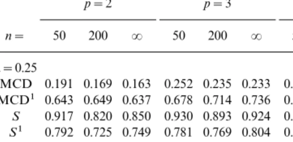
Finite-Sample Efficiencies of Off-Diagonal Elements of the MCD, S, and Reweighted MCD and S Scatter Matrix Estimators at the Normal Distribution

p=2 p=3 p=5 p=10 n= 50 200 50 200 50 200 50 200 :=0.25 MCD 0.191 0.169 0.163 0.252 0.235 0.233 0.359 0.359 0.324 0.462 0.450 0.438 MCD1 _{0.643 0.649 0.637 0.678 0.714 0.736 0.726 0.823 0.814 0.692 0.820 0.878} S 0.917 0.820 0.850 0.930 0.893 0.924 0.976 1.020 0.967 1.019 1.000 0.988 S1 _{0.792 0.725 0.749 0.781 0.769 0.804 0.846 0.879 0.849 0.941 0.909 0.891} :=0.5 MCD 0.046 0.036 0.033 0.079 0.064 0.063 0.140 0.123 0.113 0.221 0.205 0.191 MCD1 _{0.440 0.407 0.401 0.472 0.500 0.618 0.515 0.671 0.783 0.502 0.714 0.873} S 0.332 0.357 0.377 0.513 0.532 0.579 0.711 0.810 0.778 0.924 0.909 0.915 S1 _{0.697 0.667 0.682 0.730 0.735 0.767 0.803 0.850 0.842 0.904 0.905 0.890}

S-estimators have the highest efficiencies among the considered estimators:

almost always above 900 (c) reweighting an S-estimator (except for p

small and:=0.5) leads to a small loss in precision.

Since the MCD and S estimators are meant to be robust estimators of multivariate location and scatter, we compared their behavior at

con-taminated normal distributions. The generated samples contain now 200

of outliers equal tokÄe₁ whereÄe₁ is the first unit vector, while the

remain-ing 800 observations are again normally distributed. The contamination

will affect the whole scatter-matrix, and the median squared error as well as the 0.9 quantile of the squared errors (reported between parenthesis) have been computed for several values ofk. Using quantiles of the squared errors instead of the mean squared error was suggested by a referee who argued that MSEs may be misleading under this type of contamination, but the obtained results appeared to be comparable.

In Tables IX and X results for two representative cases, 7 11 and7 12, for

k=100 and kr-q$ (with$=0.025) are reported for the 250and 500

breakdown point MCD, MCD1_{, S and S}1 _{estimators. Note that k=100}

gives samples containing far away outliers which are easily detected by the robust estimators. The MCD estimator is however more sensible to inter-mediate outliers, which are much harder to detect. Some simulation

experiments indicated that kr-q$ is close to the value resulting in the

maximal squared errors one can expect for this type of contamination. One sees that the reweighted MCD remains much more precise than its initial estimator even under severe contamination and that it also outperforms the

TABLE IX

Median Squared Error and 0.9 Quantile of the Squared Errors (between Parentheses) of Element (1,1) of the MCD, S, and Reweighted MCD and S Scatter Matrix Estimators at a

200Contaminated Normal Distribution

k=100 kr-q$ p=2 p=3 p=2 p=3 : n=50 n=200 n=50 n=200 n=50 n=200 n=50 n=200 0.25 MCD 15.15 58.40 8.09 30.88 315.43 1265.97 378.75 1480.03 (64.0) (137.0) (42.9) (82.8) (540.8) (1660.4) (582.8) (1841.1) MCD1 _{1.50 2.00 1.41 1.66 62.23 248.60 106.42 405.79} (9.4) (12.6) (8.1) (9.8) (109.1) (332.2 ) (171.0) (517.9) S 611.60 2642.38 564.38 2459.76 64.63 268.39 108.62 447.09 (1225.3) (3800.6) (1146.9) (3533.5) (113.8) (360.7) (170.4) (562.2) S1 _{1.45 2.39 1.33 1.92 60.11 233.40 97.42 380.03} (9.8) (14.5) (8.8) (11.9) (102.4) (312.3) (153.2) (480.5) 0.5 MCD 10.99 26.34 9.51 18.82 1541.11 6266.32 1392.39 5281.43 (138.6) (186.4) (91.7) (121.3) (2763.5) (8574.7) (2254.7) (6888.2) MCD1 _{1.78 1.75 1.91 1.57 73.45 305.99 144.66 519.21} (9.87) (11.07) (10.48) (9.28) (145.93) (420.31) (247.74) (676.94) S 15.14 68.75 11.98 54.85 270.21 1013.36 358.03 1300.84 (67.5) (154.7) (52.8) (120.2) (616.8) (1478.7) (643.5) (1691.2) S1 _{1.53 2.04 1.40 1.80 62.83 244.80 103.84 393.80} (9.2) (12.8) (8.5) (10.6) (108.6) (329.8) (165.3) (501.9)

S-estimator in the case of extreme outliers. Although the percentage of

out-liers is close to the breakdown point of the MCD1_{estimator with :=0.25,}

the median squared error of the latter is comparable to that of the maximal

breakdown point MCD1_{. It is surprising to note that the MCD estimator}

performs better with :=0.25 than with :=0.5. The S-estimator with

:=0.25, which was the most efficient in the uncontaminated case, becomes

very unstable at the 200 contamination level. On the other hand, the

reweighted S-estimator is much more robust but does not outperform the MCD1 _{estimator. The (small) loss in efficiency paid for by reweighting the} S-estimator, is apparently compensated by a gain in robustness. This in contrast with the MCD, where the reweighted version performs better both in presence and absence of contamination.

To conclude the simulation study, one could say that reweighted S and

MCD with 250breakdown are the most appealing among all considered

estimators. Comparing MCD1 _{with S}1 _{is slightly favorable for the latter}

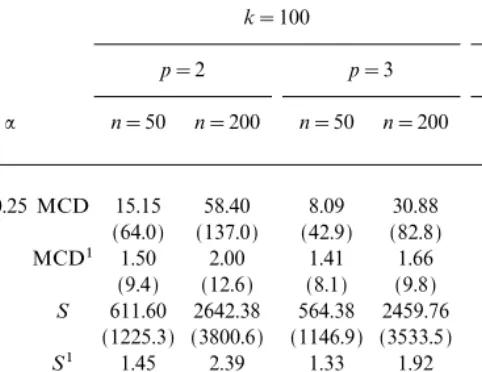
TABLE X

Median Squared Error and 0.9 Quantile of the Squared Errors (between Parentheses) of Element (1,2) of the MCD, S, and Reweighted MCD and S Scatter Matrix Estimators at a

200Contaminated Normal Distribution . k=100 kr-q$ p=2 p=3 p=2 p=3 : n=50 n=200 n=50 n=200 n=50 n=200 n=50 n=200 0.25 MCD 2.22 2.55 1.68 1.66 3.56 4.28 2.50 2.72 (13.3) (14.8) (10.0) (10.2) (21.1) (25.4) (14.8) (15.9) MCD1 _{0.73 0.73 0.68 0.67 0.79 0.83 0.80 0.71} (4.3) (4.4) (4.2) (4.1) (4.9) (4.8) (5.0) (4.3) S 11.52 12.14 11.24 11.77 0.55 0.57 0.56 0.56 (71.9) (72.2) (68.7) (71.4) (3.3) (3.2) (3.3) (3.4) S1 _{0.67 0.68 0.65 0.67 0.58 0.59 0.62 0.61} (4.2) (4.1) (4.1) (4.0) (3.7) (3.5) (3.8) (3.7) 0.5 MCD 10.02 13.17 5.60 7.04 26.90 54.99 12.83 18.80 (60.1) (76.8) (34.3) (42.0) (139.3) (289.5) (77.6) (118.2 MCD1 _{0.86 0.85 0.88 0.77 2.28 4.07 1.96 1.98} (5.2) (5.1) (5.2) (4.7) (12.3) (20.7) (11.6) (12.2) S 2.40 2.39 1.68 1.64 2.34 2.31 1.60 1.44 (14.8) (13.9) (10.7) (10.1) (18.0) (13.7) (11.1) (9.1) S1 _{0.73 0.73 0.70 0.69 0.80 0.72 0.71 0.69} (4.4) (4.2) (4.1) (4.1) (4.9) (4.2) (4.5) (3.9)

in higher dimensions. Let us not forget, however, the very intuitive

finite-sample definition of the MCD, which could make MCD1 _{more attractive}

to non-specialists in the field.

6. CONCLUSION

The development and availability of fast algorithms (Hawkins, 1994; Rousseeuw and Van Driessen, 1999) for computing the minimum covariance determinant (MCD) has brought renewed interest to this estimator. Asymptotic properties were given in Butler, Davies and Jhun (1993), but the asymptotic variance of the MCD-scatter part remained unknown. In this paper, we worked out the influence function of the MCD scatter matrix estimator and used it to evaluate the asymptotic efficiency of this robust estimator. The efficiencies of other robust estimators, whose influence function has already been derived in the literature, i.e., the

S-estimator and reweighted estimators, have also been evaluated numeri-cally.

The main conclusion is that the Gaussian efficiency of the maximal breakdown MCD estimator is rather poor, but is already substantially

higher for the 250 breakdown MCD and increases even more after

reweighting. The efficiency of the reweighted MCD with:=0.25 seems to

be acceptable: almost always above 600 in the Gaussian case, even for

finite samples.

With respect to efficiency, 250breakdown S-estimators are very attrac-tive and outperform the reweighted MCD estimators. Davies (1992b) and Lopuhaa (1991) proposed alternatives to S-estimators with a higher

efficiency, but these improvements seem only to be worthwhile in the 500

breakdown point case with p small. In spite of their positive breakdown

property, the bias of S-estimators can be considerably high. Yohai and

Maronna (1990) showed this by means of the Maxbias curve, which is a

powerful tool to quantify the robustness of an estimator. It is therefore not sufficient to consider only breakdown point and efficiency of robust estimators, also Maxbias curves should be computed. This has been done for the MCD-estimator in the univariate case (Croux and Haesbroeck, 1999), but the multivariate case seems to be rather hard to handle.

7. APPENDIX

Proof of Proposition 1. Call G=F=,x, t==T(A,y)(G), 7==7(A,y)(G) and d2

=(z)=(z&t=)t7&1= (z&t=). Define for everys>0

Es=[z#Rp|d2=(z)<s],

denote

D2_{(G)=sup[s>0 | P}

G(Es)1&:],

and take E=ED2_(G). Since lim_sÄP_G(E_s)>1&: and lim_sÄ0P_G(E_s)=< 1&:, Eis a well defined, bounded and non degenerate open ellipsoid with 1&:&=PG(E)1&:. We conclude that E#DG(:) or (E,x) #D G(:),

sincex is the only atom of the distributionG.

Consider the two following probability measures&(A,y)and&(E,x)defined

for each measurable setBby

with$=1&:&PG(A) and

&_(E,x)(B)=(P_G(E&B)+$I(x#B))(1&:),

where$ =1&:&PG(E). By definition of Eone has that $ =0, as long as

the atomx does not lie at the border of E. Therefore

$ (d2

=(x)&D

2_{(G))=0. (7.1)}

It is sufficient to show that

E_&(E,x)[d2

=(z)]E&(A,y)[d 2

=(z)]. (7.2)

Indeed, if the above equation holds, we know that there exists a 0<c1

for which

E&(E,x)[(z&t=)

t_(c7

=)&1(z&t=)]=p, (7.3)

since the RHS of (7.2), like the sum of the diagonal elements of the hat

matrix, equals p. Since (A, y) provides an MCD solution we have that

det(c7₌)det(7₌)det(7_(E,x)(G)), which in combination with (7.3) con-tradicts the result of Grubel (1988) unless t₌=T_(E,x)(G), and c7₌=

7_(E,x)(G). Then alsocshould equal 1, which will end the proof. To prove (7.2), write E_&(E,x)[d2 =(z)]= 1 1&:

{

|

E&A d2 =(z)dG(z) +

_|

E"(A_[ y]) d2 =(z)dG(z)+d 2 =(y)PG(E&[ y])+$ d2=(x)

=

. (7.4) Now

|

E"(A_[ y]) d2 =(z)dG(z)D2(G)PG(E"(A_[ y]))

=D2_{(G)(1&:&$ &P}

G(E&A)&PG(E&[ y]))

=D2_(G)(P

G(A"E)+$&$ &PG(E&[ y]))

|

A"E d2 =(z)dG(z)+D 2_{(G)($&$ &P} G(E&[ y])). (7.5)

Combining (7.4) and (7.5) with (7.1), yields E&(E,x)[d 2 =(z)] 1 1&:

{

|

A d2 =(z)dG(z) +D2_(G)($&P G(E&[ y]))+d2=(y)PG(E&[ y])

=

=E&(A,y)[d 2 =(z)]+ 1 1&:[(D 2_(G)&d2 =(y))($&PG(E&[ y]))]. (7.6) The second term of (7.5) is always negative, since D2_(G)d2

=(y) fory E

and D2_(G)d2

=(y), but $PG([ y]) fory#E. Therefore, (7.2) holds. K

Proof of Theorem1: For ease of notation, denoteF=,x0=(1&=)F+=2x0, wherex₀ is an arbitrary point, 7(F_=,x0)=7₌andT(F_=,x0)=t₌. Proposition 1 guarantees that the MCD scatter estimator atF_=,x0satisfies

7==c:

{

1 1&:

|

A(F=,x0) xxt_dF =,x0(x)&t=t t =

=

=c:

{

1&= 1&:

|

A(F=,x0) xxt_dF(x)+ = 1&:I(x0#A(F=,x0))x0x t 0&t=tt=

=

, where A(F_=,x0)=[x#Rp_{: (x&t}

=)t7&1= (x&t=)<q:(=)], for a certain

posi-tive number q:(=). (As long as &x0&2{q: one may suppose that x0 does not belong to the border of A(F=,x0) for =small, cf. Remark 4, Section 2.) By definition, IF(x0,7,F)=(7==)|==0. Let us differentiate7=w.r.t.=and set==0, 7= = |==0=c:

{

& 1 1&:

|

A(F) xxt_dF(x)+ 1 1&: =

|

A(F=,x0) xxt_dF(x) |==0 (7.7) + 1 1&:I(x0#A(F))x0x t 0

=

.

Using the Fisher consistency of 7(F) and the fact that A(F)=

[x#Rp_:xt_xq :], we get IF(x0,7,F)=&I+ c_: 1&: =

|

A(F=,x0) xxt_dF(x) |==0 + c:

1&:I(&x0&

2_q

In order to compute the second term on the right hand side of (7.8), we transform the integration variable x to y=7&12

= (x&t=). The

integra-tion domain becomes now a ball with center at the origin and radius

-q:(=). When more convenient, we will express y in polar coordinates

y=r e(%) with r# [0,-q:(=)],e(%) #Sp&1 and %=(%1, ...,%p&1) #3= [0,?[_ } } } [0,?[_[0, 2?[. The integral in (7.8), denoted byI(=), becomes

I(=)=det(712 = )

|

-q:(=) 0

|

3 J(%,r)(r712 = e(%)+t=)(r7=12e(%)+t=)t g((r712 = e(%)+t=)t(r7=12e(%)+t=))dr d%, (7.9)

whereJ(%,r) is the Jacobian of the transformation into polar coordinates. By matrix differentiation and since 7₀=I, we obtain

det(712 = ) = |==0= 1 2 det(7=) = |==0= 1 2trace (IF(x0,7,F)). (7.10)

Applying Leibniz' formula to (7.9) and using (7.10) results in I(=) = |==0= 1 2trace(IF(x0,7,F))H(q:)I+ -q_:(=) = |==0q:g(q:)d1I +

|

&y&2_q: =((7 12 = y+t=)(7=12y+t=)tg((7=12y+t=)t(71=2y+t=)))|==0dy, (7.11) with d1=3J(%,-q:)e21(%)d%=1p 3J(%,-q:)d% and H(q:)=&y&2_q

:

y2 1g(y

t_y)dy=(c

:(1&:))&1.

The derivative in the third term of (7.11) is given by =((7 12 = y+t=)(71=2y+t=)tg((7=12y+t=)t(7=12y+t=)))|==0 =1 2[IF(x0,7,F)yy t_+yyt_IF(x 0,7,F) +2IF(x0,T,F)yt+2yIF(x0,T,F)t] g(yty) +yyt_g$(yt_{y)[ y}t_IF(x 0,7,F)y+2ytIF(x0,T,F)]. (7.12) Note that since&y&2_q

:yg(y

t_y)dyand

&y&2_q

:yy

t_g$(yt_{y)y dyare zero, the}

terms in (7.12) including IF(x0,T,F) give a zero contribution to the integral in (7.11).

Equation (7.11) still depends on ((-q:(=))=)|==0 which needs to be computed. By definition ofA(F=,x0), 1&:=

|

A(F=,x0) dF_=,x 0(x)=(1&=)

|

A(F=,x0) dF(x)+=I(x₀ #A(F_=,x 0)). (7.13)

Differentiating both sides w.r.t.=yields

0=&

|

A(F)

dF(x)+

=

|

A(F=,x0)

dF(x)|== 0+I(&x0&

2_q

:). (7.14)

In the same way as before, one can easily verify that =

|

A(F=,x0) dF(x)|==0 =1&: 2 trace(IF(x0,7,F))+ -q:(=) = |==0 g(q:)

|

3 J(%,-q:)d% +

|

&y&2_q : g$(yt_y)yt_IF(x 0,7,F)y dy. (7.15)

The last term in (7.15) equals, using the symmetry of F, c₂trace(IF(x₀,

7,F)), with c₂=&y&2_q

:y

2

1g$(yty)dy.

By substituting (7.15) in (7.14), the above equation leads to -q:(=)

= |==0=

1&:&I(&x₀&2_q

:)&trace (IF(x0,7,F))(c2+(1&:)2)

g(q:)pd1

. (7.16) Inserting (7.16) and (7.12) in (7.11) gives

IF(x₀,7,F)=

&I+ c:

1&:I(&x0&

2_q :)x0xt0+ 1 2trace(IF(x0,7,F))I + c: 1&: q:

p

\

(1&:)&I(&x0&

2_q

:)&trace(IF(x0,7,F))

\

c2+ 1&:

2

++

I

+ c:

2(1&:)

|

&y&2_q

:

(IF(x0,7,F)yyt+yytIF(x0,7,F))g(yty)dy

+ c:

1&:

|

&y&2_q

:

yyt_g$(yt_y)yt_IF(x

In order to give element wise expressions for the influence function, we note that 1 2 : p k=1

{

IF(x₀,7_ik,F)

|

&y&2_q : y_ky_jg(yt_y)dy +IF(x₀,7_kj,F)

|

&y&2_q : y_iy_kg(yt_y)dy

=

=H(q:)IF(x0,7ij,F)

for every 1i, jp and

: p k=1 : p l=1 IF(x₀,7_kl,F)

|

&y&2_q : y_iy_jy_ky_lg$(yt_y)dy =

{

c3trace(IF(x0,7,F))+(c4&c3)IF(x0,7ii,F), 2c3IF(x0,7ij,F), i=j i{j,

wherec₃=&y&2_q

:y

2

iy2jg$(yty)dyand c4=&y&2_q

:y

4

ig$(yty)dy.

The constants c₂,c₃, and c₄ can be rewritten in the form given in the statement of the theorem, using polar coordinates. From (7.17) the influence function for the off-diagonal elements is immediately obtained,

IF(x0,7ij,F)=

c:x0ix0j

1&: I(&x0&

2_q

:)+

c:

1&:(2c3+H(q:))IF(x0,7ij,F),

which leads to (2.12), due to the definition ofH. For the diagonal elements, we get

IF(x0,7jj,F)=&1+

c_:x₀2

j

1&:I(&x0&

2_q :)+ 1 2trace(IF(x0,7,F)) + c: 1&: q_:

p

{

(1&:)&I(&x0&

2_q :)&trace(IF(x0,7,F))

\

c2+ 1&: 2

+=

+ c: 1&:[c4&c3+H(q:)] IF(x0,7jj,F)+ c:c3 1&:trace(IF(x0,7,F)). (7.18)

Using the constants b1 and b2 defined in Section 2, (7.18) can be written as b1IF(x0,7jj,F)&b2trace(IF(x0,7,F)) = &1+c:x 2 0j

1&:I(&x0&

2_q

:)+

c_:

1&: q_:

p [1&:&I(&x0&

2_q

:)].

(7.19) Taking the sum of the diagonal terms given in (7.19) yields the trace of the influence function

trace(IF(x0,7,F)) =(b₁&pb₂)&1_[(&c

:&x0&2(1&:))I(&x0&2q:)

+p[(c:(1&:))(q:p)(1&:&I(&x0&2q:))&1]]. (7.20)

Combining (7.19) and (7.20) gives (2.12). K

ACKNOWLEGMENTS

We thank the two referees and the editor for helpful suggestions and remarks.

REFERENCES

1. P. J. Bickel and E. L. Lehmann, Descriptive statistics for nonparametric models III, Dispersion,Ann.Statist.4(1976), 11391159.

2. R. W. Butler, Nonparametric interval and point prediction using data trimmed by a Grubbs type outlier rule,Ann.Statist.10(1982), 197204.

3. R. W. Butler, P. L. Davies, and M. Jhun, Asymptotics for the minimum covariance determinant estimator,Ann.Statist.21(1993), 13851400.

4. C. Croux and P. J. Rousseeuw, A class of high-breakdown scale estimators based on subranges, Comm.Statist.Theory Methods21(1992), 19351951.

5. C. Croux and G. Haesbroeck, ``Maxbias Curves of Robust Scale Estimators Based on Subranges,'' Technical Report, Universite Libre de Bruxelles, 1999, http:www.sig.egss. ulg.ac.beHaesbroeck.

6. P. L. Davies, Asymptotic behavior of S-estimators of multivariate location parameters and dispersion matrices,Ann.Statist.15(1987), 12691292.

7. P. L. Davies, The asymptotics of Rousseeuw's minimum volume ellipsoid,Ann.Statist.20

(1992a), 18281843.

8. P. L. Davies, An efficient Frechet Differentiable high breakdown multivariate location and dispersion estimator,J.Multivariate Anal.40(1992b), 311327.

9. R. Grubel, A minimal characterization of the covariance matrix, Metrika 35 (1988), 4952.

10. F. R. Hampel, E. M. Ronchetti, P. J. Rousseeuw, and W. A. Stahel, ``Robust Statistics: The Approach Based on Influence Functions,'' Wiley, New York, 1996.

11. D. M. Hawkins, The feasible solution algorithm for the minimum covariance determinant estimator in multivariate data, Comput.Statist.Data Anal.17(1994), 197210.

12. X. He and G. Wang, Cross-checking using the minimum volume ellipsoid estimator,

Statistica Sinica6(1996), 367374.

13. O. Hossjer and C. Croux, Generalizing univariate signed rank statistics for testing and estimating a multivariate location parameter,Nonparametric Statist.4(1995), 293308. 14. H. P. Lopuhaa, On the relation between S-estimators and M-estimators of multivariate

location and covariance,Ann.Statist.17(1989), 16621683.

15. H. P. Lopuhaa, Multivariate{-estimators for location and scatter, Canad.J.Statist.19

(1991), 307321.

16. H. P. Lopuhaa, Highly efficient estimators of multivariate location with high breakdown point,Ann.Statist.19(1992), 229248.

17. H. P. Lopuhaa, Asymptotics of reweighted estimators of multivariate location and scatter, preprint, TU Delft, 1997.

18. H. P. Lopuhaa and P. J. Rousseeuw, Breakdown properties of affine equivariant esti-mators of multivariate location and covariance matrices,Ann.Statist.19(1991), 229248. 19. R. A. Maronna and Yohai, Robust estimation of multivariate location and scatter,in

``Encyclopedia of Statistical Sciences Update'' (S. Kotz, C. Read, and D. Banks, Eds.), Vol. 2, pp. 589596, Wiley, New York, 1998.

20. D. M. Rocke, Robustness properties of S-estimators of multivariate location and shape in high dimensions,Ann.Statist.24(1996), 13271345.

21. P. J. Rousseeuw, Multivariate estimation with high breakdown point,in``Mathematical Statistics and Applications'' (W. Grossmann, G. Pflug, I. Vincze, and W. Wertz, Eds.), Vol. B, pp. 283297, Reidel, Dordrecht, 1985.

22. P. J. Rousseeuw and A. M. Leroy, ``Robust Regression and Outlier Detection,'' Wiley, New York, 1987.

23. P. J. Rousseeuw and C. Croux, The bias ofk-step M-estimators,Statist.Probab.Lett.20

(1994), 411420.

24. P. J. Rousseeuw and K. Van Driessen, A fast algorithm for the minimum covariance determinant estimator,Technometrics, to appear.

25. D. Ruppert, Computing S-estimators for regression and multivariate locationdispersion,

J.Comput.Graph.Statist.1(1992), 253270.

26. V. J. Yohai and R. A. Maronna, The maximum bias of robust covariances,Comm.Statist.