Copyright by Sungwon Lee
The Dissertation Committee for Sungwon Lee
certies that this is the approved version of the following dissertation:
Essays on Semi-/Non-parametric Methods in Econometrics
Committee:
Stephen Donald, Supervisor
Jason Abrevaya
Sukjin Han
Essays on Semi-/Non-parametric Methods in Econometrics
by
Sungwon Lee
DISSERTATION
Presented to the Faculty of the Graduate School of The University of Texas at Austin
in Partial Fulllment of the Requirements
for the Degree of
DOCTOR OF PHILOSOPHY
THE UNIVERSITY OF TEXAS AT AUSTIN May 2018
Acknowledgments
This work could not have been done without the support and encouragement from many people around me. I am deeply indebted to my advisor Stephen Donald for his guidance and support throughout my graduate life. He has provided me with many valuable lessons and the time to pursue my academic goals. I am also very grateful to Jason Abrevaya and Sukjin Han for their thoughtful discussions and suggestions. They have always helped me whenever I was in trouble and inspired me to become a good researcher. I also thank Brendan Kline, Thomas Shively, and Haiqing Xu for their sharp comments on my dissertation.
My gratitude also goes to my friends. I have beneted from discussions on my research with my research colleagues, Jessie, Peter, and Xinchen. I am sincerely grateful to other friends, Yeonjoon, Choongryul, Jaemin, Narae, David, Gabe, Joon, Eunjoo, Changseung, Haejung, Byungjae, and Jiwon.
I am grateful to my family for their support and encouragement as well. Lastly but not least, I would thank God for his guidance throughout my life.
Essays on Semi-/Non-parametric Methods in Econometrics
Publication No.
Sungwon Lee, Ph.D.
The University of Texas at Austin, 2018
Supervisor: Stephen Donald
My dissertation contains three chapters focusing on semi-/non-parametric models in econometrics. The rst chapter, which is a joint work with Sukjin Han, considers parametric/semiparametric estimation and inference in a class of bivari-ate threshold crossing models with dummy endogenous variables. We investigbivari-ate the consequences of common practices employed by empirical researchers using this class of models, such as the specication of the joint distribution of the unobserv-ables to be a bivariate normal distribution, resulting in a bivariate probit model. To address the problem of misspecication, we propose a semiparametric estimation framework with parametric copula and nonparametric marginal distributions. This specication is an attempt to ensure robustness while achieving point identication and ecient estimation. We establish asymptotic theory for the sieve maximum like-lihood estimators that can be used to conduct inference on the individual structural parameters and the average treatment eects. Numerical studies suggest the sensi-tivity of parametric specication and the robustness of semiparametric estimation.
failure of identication, unlike what some practitioners believe.
The second chapter develops nonparametric signicance tests for quantile regression models with duration outcomes. It is common for empirical studies to specify models with many covariates to eliminate the omitted variable bias, even if some of them are potentially irrelevant. In the case where models are nonparamet-rically specied, such a practice results in the curse of dimensionality. I adopt the integrated conditional moment (ICM) approach, which was developed by Bierens (1982); Bierens (1990), to construct test statistics. The proposed test statistics are functionals of a stochastic process which converges weakly to a centered Gaussian process. The test has non-trivial power against local alternatives at the parametric rate. A subsampling procedure is proposed to obtain critical values.
The third chapter considers identication of treatment eect and its distri-bution under some distridistri-butional assumptions. I assume that a binary treatment is endogenously determined. The main identication objects are the quantile treatment eect and the distribution of the treatment eect. I construct a counterfactual model and apply Manski's approach (Manski(1990)) to nd the quantile treatment eects. For the distribution of the treatment eect, I adapt the approach proposed byFan and Park(2010). Some distributional assumptions called stochastic dominance are imposed on the model to tighten the bounds on the parameters of interest. It also provides condence regions for identied sets that are pointwise consistent in level. An empirical study on the return to college conrms that the stochastic dominance assumptions improve the bounds on the distribution of the treatment eect.
Table of Contents
Acknowledgments v
Abstract vi
List of Tables xi
List of Figures xii
Chapter 1. Sensitivity Analysis in Triangular Systems of Equations
with Binary Endogenous Variables 1
1.1 Introduction . . . 1
1.2 Identication and Failure of Identication . . . 6
1.2.1 Identication. . . 6
1.2.2 The Failure of Identication . . . 10
1.2.2.1 No Exclusion Restrictions . . . 10
1.2.2.2 No Restrictions on Dependence Structures . . . 18
1.3 Estimation. . . 19
1.4 Asymptotic Theory for Semiparametric Models . . . 23
1.4.1 Consistency of the Sieve MLE . . . 25
1.4.2 Convergence Rates . . . 29
1.4.3 Asymptotic Normality a Smooth Functional . . . 31
1.4.3.1 Asymptotic normality ofψˆn. . . . 36
1.4.3.2 Asymptotic normality ofψˆnwhen the unknown marginals are equal . . . 38
1.4.3.3 Asymptotic Normality of the CATEs. . . 40
1.5 Monte Carlo Simulation and Sensitivity Analysis . . . 41
1.5.1 Simulation Design . . . 41
1.5.4 Copula Misspecication . . . 44
1.5.5 Simulation Results . . . 45
1.6 Conclusions . . . 60
Chapter 2. Nonparametric Tests for Conditional Quantile Indepen-dence with Duration Outcomes 62 2.1 Introduction . . . 62
2.1.1 Related Literature . . . 68
2.2 Model and Test Statistics . . . 70
2.3 Asymptotic theory . . . 78 2.3.1 Assumptions . . . 79 2.3.2 Weak convergence . . . 83 2.3.3 Power Properties . . . 85 2.4 Subsampling Approximation . . . 86 2.5 Conclusion. . . 90
Chapter 3. Identication and Condence Regions for Treatment Ef-fect and its Distribution under Stochastic Dominance 93 3.1 Introduction . . . 93
3.2 Previous Studies . . . 97
3.3 Identication . . . 99
3.3.1 Identication under Stochastic Dominance . . . 103
3.3.2 The Distribution of the Treatment Eect . . . 107
3.4 Estimation and Condence Regions for Identied Sets . . . 109
3.5 Application to the Return to College . . . 117
3.5.1 Data . . . 118
3.5.2 Estimation Results . . . 119
3.6 Conclusions . . . 125
Appendix A. Chapter 1 Appendix 129
A.1 Proof of Lemma 1.2.1. . . 129
A.2 Proof of Theorem 1.2.11 . . . 130
A.3 Proof of Theorem 1.4.7 . . . 133
A.4 Proof of Theorem 1.4.9 . . . 140
A.5 Proof of Proposition 1.4.1 . . . 143
A.6 Proof of Theorem 1.4.16 . . . 147
A.7 Hölder ball . . . 147
Appendix B. Chapter 2 Appendix 149 B.1 Proof of Lemma 2.2.1. . . 150 B.2 Proof of Lemma 2.2.2 . . . 151 B.3 Proof of Theorem 2.3.7 . . . 152 B.4 Proof of Theorem 2.3.8 . . . 153 B.5 Proof of Corollary 2.3.9 . . . 166 B.6 Proof of Theorem 2.3.11 . . . 167 B.7 Proof of Theorem 2.4.1 . . . 172
Appendix C. Chapter 3 Appendix 174 C.1 Proof of Lemma 3.3.1. . . 174 C.2 Proof of Lemma 3.3.2 . . . 175 C.3 Proof of Theorem 3.3.4 . . . 175 C.4 Proof of Theorem 3.3.7 . . . 176 C.5 Proof of Corollary 3.3.8 . . . 176 C.6 Proof of Theorem 3.3.10 . . . 176 C.7 Proof of Theorem 3.4.3 . . . 177 C.8 Proof of Theorem 3.4.5 . . . 179 C.9 Proof of Theorem 3.4.8 . . . 181 Bibliography 189
List of Tables
1.1 Correctly Specied Models (n= 500) . . . 49
1.2 Marginal Misspeccation (n= 500) . . . 50
1.3 Copula and Marginals Misspecication 1 (n= 500) . . . 51
1.4 Copula and Marginals Misspecication 2 (n= 500) . . . 52
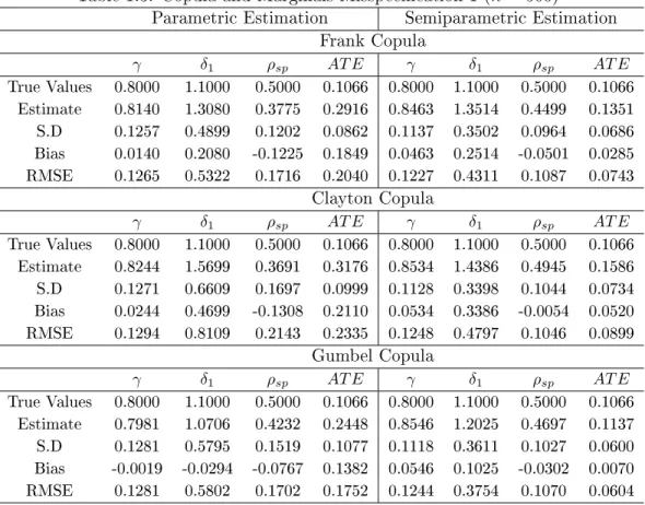
1.5 Copula and Marginals Misspecication 3 (n= 500) . . . 53
1.6 Copula and Marginals Misspecication 4 (n= 500) . . . 54
1.7 Correctly Specied Models (n= 1,000). . . 55
1.8 Marginal Misspeccation (n= 1,000). . . 56
1.9 Copula and Marginals Misspecication 1 (n= 1,000) . . . 57
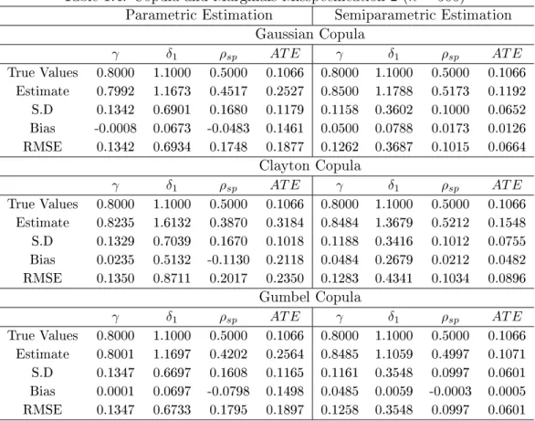
1.10 Copula and Marginals Misspecication 2 (n= 1,000) . . . 58
1.11 Copula and Marginals Misspecication 3 (n= 1,000) . . . 59
1.12 Copula and Marginals Misspecication 4 (n= 1,000) . . . 60
3.1 Descriptive Statistics . . . 121
3.2 Estimation Results of the Bounds on the QTEs . . . 122
List of Figures
1.1 A Numerical Calculation of a Distribution Function under which
Iden-tication Fails . . . 18
3.1 Bounds on the QTE under Assumption 3.3.3 . . . 122
3.2 Bounds on the QTE under Assumption 3.3.6 . . . 123
3.3 Bounds on the QTE under Assumptions 3.3.3 and 3.3.6 . . . 123
3.4 Bounds on the Distribution of the TE under Assumption 3.3.3. . . . 124
3.5 Bounds on the Distribution of the TE under Assumption 3.3.6. . . . 124
3.6 Bounds on the Distribution of the TE under Assumptions 3.3.3 and 3.3.6 . . . 125
Chapter 1
Sensitivity Analysis in Triangular Systems of Equations
with Binary Endogenous Variables
This is a joint work with Sukjin Han.
1.1 Introduction
This paper considers parametric/semiparametric estimation and inference in a class of bivariate threshold crossing models with dummy endogenous variables. LetY denote the binary outcome variable and D the observed binary endogenous treatment variable. We consider a bivariate triangular system for(Y, D):
Y =1[X0β+δ1D−ε≥0],
D=1[X0α+Z0γ−ν ≥0], (1.1.1) whereX denotes the vector of exogenous regressors that determine bothY and D, and Z denotes a vector of exogenous regressors that directly aect D but not Y (i.e., instruments forD). In this paper, we investigate the consequences of common practices employed by empirical researchers using this class of models. As important part of this investigation, we conduct a sensitivity analysis regarding the specication of the unobservables(ε, ν)'s joint distribution, which is the component of the model
is typically imposed. To address the problem of misspecication, we propose a semiparametric estimation framework with parametric copula and nonparametric marginal distributions. This specication is an attempt to ensure robustness while achieving point identication and ecient estimation.
A parametric class of models (1.1.1) includes the bivariate probit model in which the joint distribution of(ε, ν)is assumed to be a bivariate normal distribution.
This model has been widely used in empirical research such asEvans and Schwab (1995), Neal (1997), Goldman et al. (2001), Altonji et al. (2005), Bhattacharya et al. (2006), Rhine et al.(2006) and Marra and Radice (2011) to name a just few. The distributional assumption in this model, however, is made out of convenience or convention and hardly justied by underlying economic theory, thereby susceptible to misspecication. With binary endogenous regressors, the objects of interest in model (1.1.1) are mean treatment parameters besides the individual structural parameters. As the outcome variable is also binary, mean treatment parameters such as the average treatment eect (ATE) are expressed as the dierential between the marginal distributions of ε. The problem of misspecication in estimating these treatment parameters can therefore be even more severe than that in estimating individual parameters.
To one extreme, a nonparametric joint distribution of(ε, ν) can be used in
bivariate threshold crossing models as inShaikh and Vytlacil(2011). As their results suggests, however, the ATE is only partially identied in this fully exible setting. Instead of sacricing point identication, we impose a parametric assumption on
known up to a scalar parameter. At the same time, in order to ensure robustness, we allow to be unspecied the marginal distribution ofε (as well as of ν), which is involved in the calculation of the ATE. In this way, our class of models encompasses both parametric and semiparametric classes of models with parametric copula and either parametric or nonparametric marginal distributions. This broad range of models allows us to conduct a sensitivity analysis in terms of the specication of the joint distribution of(ε, ν).
The identication of the individual parameters as well as the ATE in this class of models is established in (Han and Vytlacil, 2017, hereafter HV17). They show that when the copula function for (ε, ν) satises a certain stochastic
order-ing, identication is achieved in both parametric and semiparametric models under an exclusion restriction and mild support conditions. The present paper, building on these results, considers estimation and inference in the same setting. For the semiparametric class of models (1.1.1) with parametric copula and nonparametric marginal distributions, the likelihood contains innite dimensional parameters, i.e., the unknown marginal distributions. For the estimation of this model, we consider sieve maximum likelihood (ML) estimators for the nite and innite dimensional parameters of the model as well as the functionals of them. The estimation of the parametric model is within the standard ML framework.
The contributions of this paper can be summarized as follows. This paper is intended to provide a guideline to empirical researchers through these contributions. First, we establish the asymptotic theory for the sieve ML estimators in a class of semiparametric copula-based models. This result can be used to conduct inference
on the functionals of the nite and innite dimensional parameters, such as inference on the individual structural parameters and the ATE. We show that the sieve ML estimators are consistent and their smooth functionals are root-n asymptotically normal.
Second, based on these theoretical results, we conduct a sensitivity analysis via Monte Carlo simulation studies. We nd that the parametric ML estimates can be very sensitive to the misspecication of the marginal distributions of the unob-servables. We show that, on the other hand, sieve ML estimates perform well in terms of the mean squared error (MSE) as they are robust to this misspecication, while their performance is comparable to the parametric estimates under correct specication. We also show that copula misspecication does not have substantial eects in estimation as long as the true copula is within the stochastic ordering class for identication. Since copula misspecication is a problem common to both para-metric and semiparapara-metric models, our sensitivity analysis suggests to practitioners that semiparametric consideration can be desirable in estimation and inference.
Third, we formally show that identication may fail without the exclusion restriction, unlike what is argued in Wilde (2000). The bivariate probit model is sometimes used in applied work without instruments (e.g.,White and Wolaver(2003) andRhine et al.(2006)). We show, however, that this restriction is not only sucient but also necessary for identication in parametric and semiparametric models when there is a single binary exogenous variable common to both equations. We also show that, under joint normality of the unobservables, the parameters are at best weakly
identied when there are common (possibly continuous) exogenous variables1. We
also note that another source of identication failure is the absence of restrictions on the dependence structure of the unobservables as mentioned above.
The sieve estimation method is a useful nonparametric estimation framework that allows exible specication while guarantees tractability of the estimation prob-lem; seeChen(2007) for a survey of sieve estimation in semi-nonparametric models. The estimation method is also easy to implement in practice. The sieve ML estima-tion is used in various contexts: (Chen et al.,2006, hereafter CFT06) consider the sieve estimation of semiparametric multivariate distributions that are modeled us-ing parametric copulas; Bierens (2008) applies it to the mixed proportional hazard model; Hu and Schennach (2008) and Chen et al. (2009) use the method to esti-mate nonparametric models with non-classical measurement errors. The asymptotic theory developed in this paper is based on the results established in the sieve ex-tremum estimation literature, e.g.,Chen et al. (2006);Chen(2007);Bierens (2014). A semiparametric version of bivariate threshold crossing models is also considered inMarra and Radice(2011) and Ieva et al.(2014), but unlike in the present paper, exibility is introduced for the index of the threshold and not for the distribution of the unobservables.
The paper is organized as follows. We start the next section by review-ing the identication results of HV17, and then discuss the lack of identication in the absence of exclusion restrictions and in the absence of restrictions on the
depen-1HV17 only show suciency of this restriction for identication. Mourié and Méango(2014)
show necessity of the restriction but their argument does not exploit all the information available in the model; see Section 2.2 of the present paper for details.
dence structure of the unobservables. Section1.3introduces the sieve ML estimation framework for the semiparametric class of model (1.1.1), and Section1.4establishes the large sample theory for the sieve ML estimators. The sensitivity analysis is con-ducted in Section1.5by investigating nite sample performances of parametric ML and sieve ML estimates in various dierent specications. Section1.6concludes.
1.2 Identication and Failure of Identication 1.2.1 Identication In model (1.1.1), let X (k+1)×1 ≡ (1, X1, ..., Xk) 0 and Z l×1 ≡ (Z1, ..., Zl) 0, and
conformably, letα≡(α0, α1, ..., αk)0,β ≡(β0, β1, ..., βk)0, and γ ≡(γ1, γ2, ..., γl)0.
Assumption 1.2.1. X and Z satisfy that (X, Z) ⊥(ε, ν), where ⊥ denotes sta-tistical independence..
Assumption 1.2.2. (X0, Z0) does not lie in a proper linear subspace of Rk+l a.s.2 Assumption 1.2.3. There exists a copula functionC : (0,1)2 →(0,1)such that the
joint distributionFεν of (ε, ν)satises Fεν(ε, ν) =C(Fε(ε), Fν(v)), where FεandFν are marginal distributions of ε and ν, respectively, that are strictly increasing and absolutely continuous with respect to Lebesgue measure.3
Assumption 1.2.4. As scale and location normalizations, α1 =β1 = 1 and α0 =
β0= 0.
2A proper linear subspace of
Rk+lis a linear subspace with a dimension strictly less thank+l.
The assumption is that, ifM is a proper linear subspace ofRk+l, thenPr[(X0, Z0)∈M]<1.
A model with alternative scale and location normalizations,V ar(ε) =V ar(ν) = 1 and E[ε] =E[ν] = 0, can be seen as a reparametrized version of the model with
the normalizations in Assumption 1.2.4; see e.g., the reparametrization (1.2.1) be-low. For x ∈ supp(X) and z ∈ supp(Z), write a one-to-one map (by Assumption
1.2.3) as
sxz ≡Fν(x0α+z0γ),
r0,x≡Fε(x0β), (1.2.1)
r1,x≡Fε(x0β+δ1).
Take (x, z) and (x,z˜) for some x ∈ supp(X|Z = z) ∩ supp(X|Z = ˜z) where
supp(X|Z) is the conditional support of X given Z. Then by Assumption 1.2.1, model (1.1.1) implies that the tted probabilities are written as
p11,xz =C(r1,x, sxz), p11,xz˜=C(r1,x, sxz˜), p10,xz =r0,x−C(r0,x, sxz), p10,xz˜=r0,x−C(r0,x, sx˜z), (1.2.2) p01,xz =sxz−C(r1,x, sxz), p01,xz˜=sx˜z−C(r1,x, sxz˜),
wherepyd,xz ≡Pr[Y =y, D = d|X =x, Z = z] for (y, d) ∈ {0,1}2. The equation
(1.2.2) serves as the basis for identication and estimation of the model. Depending upon whether one is willing to impose an additional assumption on the dependence
structure of the unobservables (ε, ν) via C(·,·), the underlying parameters of the
model is either point identied or partially identied.
We rst consider point identication. The results for point identication can be found in HV17, which we adapt here given Assumption 1.2.4. The additional dependence structure can be characterized in terms of the stochastic ordering of the copula parametrized with a scalar parameter.
Denition 1.2.5 (Strictly More SI or Less SD). Let C(u2|u1) and C˜(u2|u1) be
conditional copulas, for which 1−C(u2|u1) and 1−C˜(u2|u1) are either increasing
or decreasing inu1 for all u2. Such copulas are called to be stochastically increasing
(SI) or stochastically decreasing (SD), respectively. Then C˜ is strictly more SI (or
less SD) thanC ifψ(u1, u2)≡C˜−1(C(u2|u1)|u1) is strictly increasing in u1,4 which
is denoted asC≺S C˜.
This ordering is equivalent to having a ranking in terms of the rst order stochastic dominance. Let (U1, U2) ∼ C and ( ˜U1,U˜2) ∼ C˜. When C˜ is strictly
more SI (less SD) than C, then Pr[ ˜U2 > u2|U˜1 = u1] increases even more than Pr[U2> u2|U1 =u1]asu1 increases.5
Assumption 1.2.6. The copula in Assumption1.2.3satisesC(·,·) =C(·,·;ρ)with
a scalar dependence parameter ρ ∈ Ω, is twice dierentiable in u1, u2 and ρ, and
satises
C(u1|u2;ρ1)≺S C(u1|u2;ρ2) for any ρ1 < ρ2. (1.2.3)
4Note thatψ(u
1, u2)is increasing inu2by denition.
The meaning of the last part of this assumption is that the copula is ordered inρ in the sense of the stochastic ordering dened above. This requirement denes a class of copulas that we allow for identication. Many well-known copulas sat-isfy (1.2.3): the normal copula, Plackett copula, Frank copula, Clayton copula and many more; see HV17 for the full list of copulas and their expressions. Under these assumptions, we rst discuss the identication in a fully parametric model:
Assumption 1.2.7. Fε and Fν are known with means µ ≡(µε, µν) and variances
σ2 ≡(σε2, σν2).
Given this assumption, Fν(ν) =Fν˜(˜ν) and Fε(ε) = Fε˜(˜ε) where Fν˜ and Fε˜
are the distributions ofν˜≡(ν−µν)/σν and ε˜≡(ε−µε)/σε, respectively. Dene
X≡ [
z0γ6=˜z0γ z,z˜∈supp(Z)
supp(X|Z=z)∩supp(X|Z = ˜z).
Theorem 1.2.8. In model (1.1.1), suppose Assumptions 1.2.11.2.7 hold. Then
(α0, β0, δ1, γ, ρ, µ, σ)are point identied in an open and convex parameter space if (i)
γ is a nonzero vector; and (ii)X does not lie in a proper linear subspace of Rk a.s. The proofs of this theorem is minor modication of the proof of Theorem 5.1 in HV17.
Although the parametric structure on the copula is necessary for point iden-tication of the parameters, HV17 show that the parametric assumption forFε and Fν are not necessary. Additionally, if we make a large support assumption, we can also identify the nonparametric marginal distributionsFε and Fν.
Assumption 1.2.9. (i) The distributions ofXj (for1≤j≤k) andZj (for1≤j≤ l) are absolutely continuous with respect to Lebesgue measure; (ii) There exists at least one elementXj inX such that its support conditional on(X1, ..., Xj−1, Xj+1, ..., Xk) isR andαj 6= 0 andβj 6= 0, where, without loss of generality, we let j= 1.
Theorem 1.2.10. In model (1.1.1), suppose Assumptions1.2.11.2.6, and 1.2.9(i) hold. Then(α0, β0, δ1, γ, ρ)are point identied in an open and convex parameter space
if (i)γ is a nonzero vector; and (ii)Xdoes not lie in a proper linear subspace of Rk a.s. Additionally, if Assumption 1.2.9(ii) holds, Fε(·) andFν(·) are identied up to
additive constants.
An interesting function of the underlying parameters that are point identi-ed in under the parametric and semiparametric distributional assumptions is the conditional ATE:
AT E(x) =E[Y1−Y0|X =x] =Fε(x0β+δ1)−Fε(x0β). (1.2.4) 1.2.2 The Failure of Identication
In this section, we discuss two sources of identication failure, namely, the absence of exclusion restrictions and the absence of restrictions on the dependence structure of the unobservables(ε, ν).
1.2.2.1 No Exclusion Restrictions
papers relies on Wilde (2000), which provides an identication argument of count-ing the number of equations and unknowns in the system. Here we show that this argument is insucient for identication. We show that without excluded instru-ments, i.e., when γ = 0, the structural parameters are not identied even with full
parametric specication of the joint distribution (Assumptions1.2.6and1.2.7). The existence of common exogenous covariates X in both equations is not very helpful for identication in a sense that becomes clear below.
Before considering the lack of identication in a general case with possibly continuous X1 inX = (1, X1), we start the analysis with binaryX1. Mourié and Méango(2014) show the lack of identication when there is no excluded instrument in the bivariate probit model with binary X1. They, however, only provide a
nu-merical counter-example. Moreover, their analysis does not consider the full set of observed tted probabilities, and hence possibly neglects information that could have contributed for identication. Here we provide an analytical counter-example in a more general parametric class of model (1.1.1) that nests the bivariate probit model. We shows that there exists two distinct values of (δ1, ρ, µε, σε) that generate the same observed tted probabilities, even if the full set of probabilities are used. Note that the reduced-form parameters (µν, σν) are always identied from the equation
forD, and α=β = (0,1)0 as normalization with scalar X1.
Theorem 1.2.11. In model (1.1.1) withX= (1, X1)whereX1 ∈supp(X1) ={0,1},
suppose that the assumptions in Theorem 1.2.8 hold, except that γ = 0. Then there
exist two distinct sets of (δ1, ρ, µε, σε) that generate the same observed data.
induced byC(u1, u2) is symmetric aroundu2 =u1 andu2 = 1−u1, and the density
induced by Fε is symmetric. Note that the bivariate normal distribution, namely, the normal copula with normal marginals, satises these symmetry properties. That is, in the bivariate probit model with a common binary exogenous covariate and no excluded instruments, the structural parameters are not identied.
Under Assumption 1.2.4, let
q0 ≡Fν˜(−µν/σν), q1 ≡Fν˜((1−µν)/σν), t0 ≡Fε˜(−µε/σε), t1 ≡Fε˜((1−µε)/σε), we have ˜ p11,0=C(Fε˜(Fε˜−1(t0) +δ1), q0;ρ), ˜ p11,1=C(Fε˜(Fε˜−1(t1) +δ1), q1;ρ), ˜ p10,0=t0−C(t0, q0;ρ), ˜ p10,1=t1−C(t1, q1;ρ), ˜ p00,0= 1−t0−q0+C(t0, q0;ρ), ˜ p00,1= 1−t1−q1+C(t1, q1;ρ),
where pyd,x˜ ≡ Pr[Y = y, D = d|X1 = x]. We want to show that, given (q0, q1)
that generate the same observed tted probabilities pyd,˜ 0 and pyd,˜ 1 for all (y, d) ∈ {0,1}2. In showing this, the following lemma is useful:
Lemma 1.2.1. Assumption1.2.6implies that, for any (u1, u2)∈(0,1)2 andρ∈Ω,
Cρ(u1, u2;ρ)>0. (1.2.5)
The proofs of this lemma and other results below are collected in the Ap-pendix.
Now x (q0, q1) ∈(0,1)2. First, consider the tted probability p˜10,0. Given
t0 ∈(0,1)andρ∈Ω, note that, forρ∗ > ρ6, there exists a solutiont∗0=t∗0(t0, q0, ρ, ρ∗)
such that
t0−C(t0, q0;ρ) = Pr[u1 ≤t0, u2≥q0;ρ] (1.2.6) = Pr[u1 ≤t∗0, u2≥q0;ρ∗] (1.2.7) =t∗0−C(t∗0, q0;ρ∗),
and note that by Assumption 1.2.6 and a variant of Lemma 1.2.1, we have that t∗0 > t0. Here, (t0, q0, ρ) and (t∗0, q0, ρ∗) result in the same observed probability ˜
p10,0 =t0−C(t0, q0;ρ) =t0∗−C(t∗0, q0;ρ∗). Now consider the tted probabilityp˜11,0.
Chooseδ1= 0. Also let Fε˜∼U nif(0,1)only for simplicity, which is relaxed in the
6The inequality here and other inequalities implied from this (e.g.,t∗
0> t0, and etc.) are assumed
Appendix. Then there exists a solutiont†0 =t†0(t0, q0, ρ, ρ∗) such that
C(t0, q0;ρ) = Pr[u1≤t0, u2 ≤q0;ρ] (1.2.8) = Pr[u1≤t†0, u2 ≤q0;ρ∗] (1.2.9) =C(t†0, q0;ρ∗),
and note that t†0 < t0 by Assumption 1.2.6 and Lemma 1.2.1. Then, by letting
δ∗1 =t†0−t∗0,(t0, q0, δ1, ρ)and (t∗0, q0, δ∗1, ρ∗) satisfy p˜11,0 =C(t0+ 0, q0;ρ) =C(t∗0+
δ∗1, q0;ρ∗). Lastly, note that p˜00,0 = 1−q0−p˜10,0 and p˜01,0 = q0 −p˜11,0, and so (t0, δ1, ρ) and (t∗0, δ∗1, ρ∗) above will also result in the same values ofp˜00,0 and p˜01,0.
It is tempting to have a parallel argument forp˜10,1,p˜11,1,p˜00,1, andp˜01,1, but
there is a complication. Although other parameters are not, δ1 and ρ are common
in both sets of probabilities. Therefore, we proceed as follows. First, considerp˜10,1.
Givent1 ∈ (0,1)and the above choice of ρ∗ ∈ Ω, note that there exists a solution
t∗1 =t∗1(t1, q1, ρ, ρ∗) such that
t1−C(t1, q1;ρ) = Pr[u1 ≤t1, u2≥q1;ρ] (1.2.10) = Pr[u1 ≤t∗1, u2≥q1;ρ∗] (1.2.11) =t∗1−C(t∗1, q1;ρ∗),
and similarly as before, we have t∗1 > t1. Here, (t1, q1, ρ) and (t∗1, q1, ρ∗) result in
the same observed probability p˜10,1 = t1 −C(t1, q1;ρ) = t∗1 −C(t∗1, q1;ρ∗). Now
t†1 =t†1(t1, q1, ρ, ρ∗) such that
C(t1, q1;ρ) = Pr[u1≤t1, u2 ≤q1;ρ] (1.2.12) = Pr[u1≤t†1, u2 ≤q1;ρ∗] (1.2.13) =C(t†1, q1;ρ∗),
and thust†1< t1. Then, if we can show that
t†1=t∗1+δ1∗, (1.2.14) where t∗1 and δ1∗ are the values already determined above, then (t1, q1, δ1, ρ) and (t∗1, q1, δ1∗, ρ∗) result in p˜11,1 = C(t1+ 0, q1;ρ) = C(t∗1+δ1∗, q1;ρ∗). Then similar as
before, the two sets of parameters will generate the same values ofp˜00,1 = 1−q1−p˜10,1
and p˜01,1 = q1 −p˜11,1. Consequently, (t0, t1, q0, q1, δ1, ρ) and (t∗0, t∗1, q0, q1, δ∗1, ρ∗)
generate the same entire observed tted probabilities. The remaining question is whether we can nd(t0, t1, δ1, ρ) and (t∗0, t∗1, δ1∗, ρ∗) such that (1.2.14) holds; this is
shown in the Appendix whereFε˜∼U nif(0,1)is also relaxed.
One might argue that the lack of identication in Theorem 1.2.11is due to the limited variation ofX. Although it is a plausible conjecture, this does not seem to be the case with the model considered in this paper.7 We now consider a general
case with possibly continuous X1 and discuss what can be said about the existence
of two distinct sets of(β, δ1, ρ, µε, σε)that generate the same observed data. To this
7In fact, in Heckman(1979)'s sample selection model under normality, although identication
fails with binary exogenous covariates in the absence of exclusion restriction, it is well-known that identication is achieved with continuous covariates by exploiting the nonlinearity of the model (Vella(1998)).
end, dene q(x)≡Fν˜((x0α−µν)/σν), t(x)≡Fε˜((x0β−µε)/σε), and then p11,x=C(Fε˜(Fε˜−1(t(x)) +δ1), q(x);ρ), p10,x=t(x)−C(t(x), q(x);ρ), p00,x= 1−t(x)−q(x) +C(t(x), q(x);ρ).
Similar to the proof strategy for the binaryX1 case, we want to show that, given
(α, µν, σν), there are two distinct sets of parameter values(β, δ1, ρ, µε, σε)and(β∗, δ∗1, ρ∗, µ∗ε, σε∗) that generate the same observed tted probabilitiespyd,x for all (y, d)∈ {0,1}2 and
x∈supp(X).
Let t(x) ≡ Fε˜(x0β) ∈ (0,1) for all x and for some β. Also, choose δ1 = 0
and someρ ∈ Ω. For ρ∗ > ρ, we will show that there exists (β∗, δ1∗) such that, for
t∗(x)≡Fε˜(x0β∗),
p10,x=t(x)−C(t(x), q(x);ρ) =t∗(x)−C(t∗(x), q(x);ρ∗) (1.2.15) p11,x=C(Fε˜(Fε˜−1(t(x)) + 0), q(x);ρ) =C(s†(x), q(x);ρ∗) (1.2.16)
for allx, where
simultaneously hold. First note that, sinceρ∗ > ρ,t∗ > t and henceβ∗ 6=β by the assumption that there is no linear subspace in the space of X. Now as before, take C(·,·;ρ) to be a normal copula and choose ρ = 0 and ρ∗ = 1. Then by arguments
similar to the binary case, we obtain
t∗(x) =q(x) + (1−q(x))t(x), (1.2.18) ands†(x) =q(x)t(x). Then (1.2.17) can be rewritten as
δ1∗=Fε˜−1(s†(x))−Fε˜−1(t∗(x))
=Fε˜−1(q(x)t(x))−Fε˜−1(q(x) + (1−q(x))t(x)). (1.2.19)
The complication here is to make this equation satised for allx. Note that (1.2.18) and (1.2.19) are consistent with the denition of a distribution function of a continuous r.v.: Fε˜(+∞) = 1, Fε˜(−∞) = 0, and Fε˜(ε) is strictly increasing.
We can then numerically show that a distribution function that is close to a normal distribution satises the conditions with a particular choice of(β∗, δ∗1); see Figure1.1.
This gure compares that distribution function (blue line) to a normal distribution function (green line).
Although, no formal derivation of counterexample is given, this result sug-gests the following: (i) In the bivariate probit model with continuous common exoge-nous covariates and no excluded instruments, the parameters will be at best weakly identied; (ii) This also implies that the structural parameters and the marginal distributions of the semiparametric model considered in Theorem 1.2.10 are not
Figure 1.1: A Numerical Calculation of a Distribution Function under which Iden-tication Fails
identied without an exclusion restriction even ifX1 has large support.
1.2.2.2 No Restrictions on Dependence Structures
When the restriction imposed onC(·,·)(i.e., Assumption1.2.6) is completely
relaxed, the underlying parameters of model (1.1.1) may fail to be identied whether or not the exclusion restriction holds. That is, a structure on how the unobservables
(ε, ν) are dependent to each other is necessary for identication. This is closely
related to the results in the literature that the treatment parameters (which is a lower dimensional function of the individual parameters) in triangular models similar to (1.1.1) is only partially identied without distributional assumptions; see Bhat-tacharya et al. (2008), Chiburis (2010), Shaikh and Vytlacil (2011), and Mourié
Suppose Assumptions1.2.11.2.4hold. Then the model becomes a semipara-metric threshold crossing model in that the joint distribution is completely unspec-ied. Then as a special case of Shaikh and Vytlacil (2011), one can easily derive bounds for the ATEFε(x0β+δ1)−Fε(x0β). The sharpness of these bounds is shown
in their paper under a rectangular support assumption for(X, Z), which in turn is
relaxed inMourié(2015). Additionally with Assumption1.2.7, one can also derive bounds for the individual parametersx0β andδ1, as it is shown in Chiburis(2010).
When there is no excluded instruments in the model,Chiburis(2010) shows that the bounds on the ATE do not improve over Manski(1990)'s bounds, which argument applies for the individual parameters.
1.3 Estimation
Let Wi ≡ (Yi, Di, Xi0, Zi0)0 be an observation of individual i and let w be a realization of Wi. We denote the supports of W, , and ν by SW, S, and Sν, re-spectively. We assume that the distribution functionsF and Fν admit the density functionsf andfν, respectively. Then we can deneθ≡(ψ0, f, fν)0 as the
param-eter of the model. The paramparam-eter space needs to be dened carefully. Since we want the density functions f and fν to be nonnegative, we dene the parameter spaces off and fν by using square root density functions. That is, we consider
Fj ={f =g2 :g∈F, Z
{g(x)}2dx= 1}, (1.3.1)
wherej ∈ {, ν} and F is a space of functions, which will be specied later, as the parameter space of fj . Then we can dene Θ˜ ≡ Ψ˜ ×F×Fν as the parameter
space ofθ. Note that, by dening θas the parameter of the model, we can consider F() = RS1[t ≤ ]f(t)dt and Fν(ν) = RSν1[t ≤ν]fν(t)dt as functionals of θ. To distinguish an element θ ∈ Θ˜ from the true parameter, let θ0 = (ψ
0
0, f0, fν0)
0
∈ Θ˜
be the true parameter.
We adopt the maximum likelihood (ML) method to estimate the parameters in the model. Assuming that the data are i.i.d, we dene the conditional density function of(Yi, Di)on (Xi0, Zi0)0 as
f(Yi, Di|Xi, Zi;θ) = Q y,d=0,1
[pyd(Xi, Zi;ξ)]1{Yi=y,Di=d},
wherepyd(x, z;ξ) abbreviates the right hand side expression that equates pyd,xz in (1.2.2) andf(y, d|x, z;θ) is the conditional density of(Yi, Di) on(X
0 i, Z 0 i) = (x 0 , z0).
Then the log of densityl(θ, w)≡logf(y, d|x, z;θ)becomes
l(θ, Wi)≡ P y,d=0,1
1yd(Yi, Di)·logpyd(Xi, Zi;θ), (1.3.2) where1yd(Yi, Di) ≡1{Yi =y, Di =d}. Then the ML estimator of θ0, θ˜n, is dene
as ˜ θn≡arg max θ∈Θ˜ Qn(θ), (1.3.3) whereQn(θ) = n1 n P i=1
l(θ, Wi) is the log-likelihood function.
Since functionl(θ, Wi)contains both nite-dimensional and innite-dimensional
parameters, it is not easy to solve the optimization problem in Equation (1.3.3) with-out additional information on f and fν. If the innite-dimensional parameters f and f are fully characterized by nite-dimensional parameters, say η ≡(η0, η0)0 ∈
H ⊂ Rdη for some integer dη > 0, then the estimator θn˜ becomes a standard ML estimator. For example, if one imposes Assumption 1.2.7, then η = (µ, σ)0 and
ην = (µν, σν)0. This parametrization leads us to redene the parameter θ and the parameter spaceΘ˜ asθ= (ψ0
, η0)0 ∈Ψ˜ ×H⊂Rdψ+dη andΘ˜ ≡Ψ˜ ×H, and the ML
estimatorθ˜nis obtained by maximizingQn(θ)over the parameter spaceΘ = ˜˜ Ψ×H.
One can show that the parametric ML estimator θ˜n is consistent, asymptotically
normal, and ecient under some regularity conditions, and those conditions are provided by, for example, Newey and McFadden (1994).
Although the parametric ML estimator possesses many desirable proper-ties, the model needs to be correctly specied to guarantee that those properties of the ML estimator hold. Since most of economic theories do not suggest choice of distributions, people have tried to seek for more robust estimation methods to misspecication. In this paper, we adopt the sieve method to estimate the unknown density functions to obtain robustness and exibility of the model.
Let Fεn and Fνn be appropriate sieve spaces for Fε and Fν, respectively, and let fn(·;an) and fνn(·;aνn) be the sieve approximations of f and fν on their sieve spaces Fn andFνn, respectively. Then we dene the sieve ML estimatorθˆn as following : ˆ θn≡arg max θ∈Θ˜n Qn(θ), (1.3.4) where Θ˜n≡Ψ˜ ×Fn×Fνn.
from the following unconstrained optimization problem: max ψ,an n P i=1 l(ψ, an, Wi)−λnPen(an)+τε 1− Z Sεfε(t, an)dt +τν 1− Z Sνfν(t, aνn)dt , wherean = (a0n, aνn0 )0, l(Wi, ψ, an) is the log likelihood with sieve approximations
fε(·, an)andfν(·, aνn), Pen(an) is the penalization term that imposes, for example,
the properties of Holder space, and the remaining penalization terms are to impose the properties of a density function. Note thatτε>0 and τν >0.
We are interested in a class of smooth univariate densities and focus on approximation of a square root density. Specically, we assume that√f and √fν belong to the class of p-smooth functions8and we restrict our attention to the linear
sieve spaces for F and Fν. In this case, the choice of sieve spaces for F and Fν depends onS and Sν, respectively. If the supports are bounded, then one can use the polynomial sieve, the trigonometric sieve, or the cosine sieve. When the supports are unbounded, then we can use the Hermite polynomial sieve or the spline wavelet sieve to approximate a square root density.
We conne our attention to cases where the copula function is correctly specied for establishing the asymptotic theory. Since the copula is specied by some nite-dimensional parameter, the model is vulnerable to misspecication of the copula function. It is well-known that if the density function is misspecied in a ML problem, the ML estimator converges to a pseudo-true value which minimizes the Kullback-Leibler Information Criterion (KLIC) (e.g. White (1982), Chen and Fan
(2006a) andChen and Fan(2006b)). We do not pursue investigating the asymptotic properties of the sieve estimators under copula misspecication, but there are several tests that can be useful to check misspecication of the copula in some classes of models. Chen and Fan (2006a) propose a test procedure for model selection, which is based on the test of Vuong (1989). Liao and Shi (2017) extend Vuong's test to the one for models containing innite dimensional parameters and propose a uniformly asymptotically valid Vuong test for semi/non-parametric models. Their setting encompasses the models that can be estimated by the sieve ML as a special case, so one may refer to the paper for model selection in our context. Even if we assume that the copula function is correctly specied to develop the asymptotic theory, we address the issue on misspecication of the copula in part by conducting some simulations to see how misspecication of copula aects the performance of estimators.
1.4 Asymptotic Theory for Semiparametric Models
In this section, we provide the asymptotic theory for the sieve ML estimator. We slightly modify the model to investigate the asymptotic properties of the sieve M-estimator. Specically, we consider the following specication:
F0(x) =H0(G(x))
Fν0(x) =Hν0(Gν(x)), (1.4.1)
whereH0(·) and Hν0(·)are unknown distribution functions on [0,1]and G(·) and
possible that G(·) and Gν(·) are dierent from each other, but this is not crucial
when it comes to estimating the parameters in the model as the main diculty with estimation relies on the unknown functions H0 and Hν0. We assume that
G(·) = Gν(·) ≡G(·) to avoid the complexity of notations. The transformation in
Equation (1.4.1) can be found in the literature (e.g. Bierens(2014)) and we do not have any loss of generality. Furthermore, the transformation may make it easier to derive the asymptotic properties of the estimator because the unknown innite-dimensional parameters are dened on a bounded set. For the known distribution function G, we can choose G(x) ≡ Φ(x) for x ∈ R, where Φ(·) is the standard
normal distribution function, and assume that H0(·) and Hν0(·) have their density
functionsh0(·)andhν0(·), respectively, on[0,1]. With this modication, we redene
the parameter as θ= (ψ0, h0, hν0)
0
∈Θ˜†, where Θ˜†= ˜Ψ×H×Hν, and the sieve space becomes Θ˜†
n= ˜Ψ×Hn×Hνn.
LetGbe a mapping fromRto [0,1], which is strictly increasing onR. Then one may wonder if there existH0 and Hν0 satisfying (1.4.1). Since G is assumed
to be strictly increasing, there exists its inverse function G−1. Letting H0(·) =
F0(G−1(·)) and Hν0(·) = Fν0(G−1(·)), it is straightforward to see that H0 and
Hν0 are mapping from [0,1]to [0,1]and satisfying the relations in (1.4.1). We also
note that such a transformation does not change identication results. SinceG(·) is
strictly increasing onR, it has the inverse functionG−1(·). Then it is straightforward
to show that, with the transformation given by Equation (1.4.1),H0(·) =F0(G−1(·))
and thusF0is identied onRif and only ifH0is identied on[0,1]. Assuming thatG
above, the unknown density functionh0 can be written ash0(x) = f0(G
−1(x))
g(G−1(x)), where
g(x) = dGdx(x). This expression draws the conclusion thatf0is identied if any only if
h0(x)is identied. Hence, we can conclude thath0andhν0 are identied if and only
if the unknown marginal density functionsf0 and fν0 are identied and G admits
the density g on R. Therefore, we choose G such that G is dierentiable and that the derivative, denoted byg, is bounded away from zero on R. It is clear that using
ΦasGsatises those requirements.
1.4.1 Consistency of the Sieve MLE
The consistency of the sieve ML estimator has been established in several papers (e.g. Geman and Hwang (1982); Gallant and Nychka (1987); White and Wooldridge(1991); Bierens (2014)). Chen (2007) provides sucient conditions un-der which the sieve M-estimator is consistent, and we establish the consistency by verifying the conditions in Theorem 3.1 inChen (2007).
We redene the parameter space to facilitate developing the asymptotic the-ory. The identication requires the space of the nite-dimensional parameterΨ˜ to
be open and convex (see Theorems 1.2.8 and 1.2.10), and thus Ψ˜ cannot be
com-pact. We introduce an optimization space which contains the true parameter ψ0
and consider it as the parameter space of ψ. Formally, we restrict the parameter space for estimation in the following way.
Assumption 1.4.1. There exists a compact and convex subset Ψ ⊆ Ψ˜ such that
ψ0 ∈int(Ψ), where int(A) is the interior of a set A.
Hν and the corresponding sieve space is denoted byΘn≡Ψ×Hn×Hνn. Then the sieve ML estimator in Equation (1.3.4) is also redened as following :
ˆ
θn≡arg maxθ∈ΘnQn(θ) (1.4.2)
DeneQ0(θ)≡E[l(θ, Wi)]and let || · ||c be a norm onΘ, whose the form is of||θ||c≡ ||ψ||E+||h||H+||hν||Hν, where || · ||E is the Euclidean norm and || · ||H and|| · ||Hν are norms on H andHν, respectively. Letdc(·,·) : Θ×Θ→[0,∞) be a pseudo metric induced by the norm|| · ||c.
We introduce some classes of functions to dene the parameter space. Let
Cm(X) be the space of m-times continuously dierentiable real-valued functions on
X. Letζ ∈(0,1]and, given ad-tupleω, let[ω] =ω1+...+ωd. Denote the dierential
operator byD and let Dω = ∂[ω]
∂xω1 1 ...∂x
ωd d
. Letting p = m+ζ, we dene the Hölder norm for h∈Cm(X) as following :
||h||Λp ≡ sup [ω]≤m,x |Dωh(x)|+ sup [ω]=m sup x,y∈X,||x−y||E6=0 |Dωh(x)−Dωh(y)| ||x−y||ζE <∞, whereζ is the Hölder exponent. We dene a Hölder class as Λp(X)≡ {h∈Cm(X) : ||h||Λp < ∞}. A Hölder ball with radius R, Λp
R(X), is dened as Λ p
R(X) ≡ {h ∈
Λp(X) :||h||Λp≤R <∞}.
We rst need to choose the norms|| · ||H and|| · ||Hν onH andHν, respec-tively, to prove the consistency. It is important to choose appropriate norms to ensure compactness of the original parameter space as compactness plays an important role in establishing the asymptotic theory. Since the parameter space contains innite
dimensional spaces, the parameter space may be compact under certain norms and may not be compact under other norms. Since closedness and boundedness of an innite dimensional space are no longer equivalent to compactness, it is much harder to show that the parameter space is compact under certain norms. To overcome this diculty, we take the approach introduced byGallant and Nychka(1987), which uses two norms to obtain the consistency. Their idea is to use the strong norm to dene the parameter space as a ball and then obtain compactness of the parameter space by equipping another norm, the consistency norm. Freyberger and Masten (2015) recently extend the idea to more cases and present compactness results for several parameter spaces. Note that, using the transformation of the distribution functions in Equation (1.4.1), the unknown innite dimensional parameters are dened on bounded domains.
We present assumptions under which the sieve ML estimator in Equation (1.4.2) is consistent with respect to some pseudo-metricdc(·,·).
Assumption 1.4.2. There exists a measurable function p(X, Z) such that for all
θ ∈ Θ and for all y, d = 0,1, pyd,XZ(θ) ≥ p(X, Z) with E|log(p(X, Z))| < ∞ and E[p(X,Z1 )2]<∞.
Assumption 1.4.3. (Wi)ni=1 are i.i.d. andE[||(X 0 i, Z 0 i) 0 ||2 E]<∞. Assumption 1.4.4. (i) √h0, √
hν0 ∈ ΛpR([0,1]) with p > 12 and some R >0; (ii) H={h =b2 :b∈ΛpR([0,1]),R01h = 1}, where R is the same to the one in (i), and
H =Hν =H; (iii) the density functions h0 and hν0 are bounded away from zero
Assumption 1.4.5. (i)Hn=Hνn={h∈H :h(x) =pkn(x) 0
akn, akn ∈R
kn,||h||
∞< 2R2}, where kn → ∞ and kn/n → 0 as n → ∞; (ii) For all j ≥ 1, we have Θj ⊆Θj+1 and there exists sequence{πjθ0}j such that dc(πjθ0, θ0)→0 asj → ∞.
Assumption 1.4.6. Forj = 1,2, denoteCj(u1, u2;ρ)≡ ∂C(u∂u1,uj2;ρ)andCρ(u1, u2;ρ)≡
∂C(u1,u2;ρ)
∂ρ . The derivatives Cj(·,·;·) and Cρ(·,·;·) are uniformly bounded for all j = 1,2.
Assumption1.4.2guarantees that the log-likelihood functionl(θ, Wi)is
well-dened for allθ ∈ Θ and that Q0(θ0) > −∞. Assumption 1.4.3 restricts the data
generating process and assumes existence of moments of the data. Assumption1.4.4 denes the parameter space and implies that the innite dimensional parameters are in some smooth class. Note that the conditions (i) and (ii) in Assumption1.4.4 together imply thath0andhν0belong toΛpR˜([0,1])whereR˜≡2m+1R2<∞9. Thus,
we may assume thath0 and hν0 belong to a Hölder ball with smoothness p under
Assumption1.4.4. While the condition (i) implicitly denes the strong norm (Hölder norm), Assumption 1.4.4-(iv) denes the sup-norm as the weak norm (consistency norm). Note that since the parameter space for the nite-dimensional parameterψ,
Ψ, is assumed to be compact in Assumption 1.4.1, the whole parameter spaceΘ is
compact under the||· ||cby Theorems 1 and 2 inFreyberger and Masten(2015). The rst part of Assumption1.4.5restricts our choice of sieve spaces forH andHν to be among linear sieve spaces with orderkn, and this can be relaxed so that the choice of kn is dierent for h and hν. The latter part of Assumption 1.4.5 requires that
the sieve space should be appropriately chosen so that the unknown parameters can be well-approximated. Since the unknown innite-dimensional parameters belong to a Hölder ball and they are dened on bounded supports, one may choose the polynomial sieve, the trigonometric sieve, the cosine sieve, or the spline sieve 10.
For example, if we choose the polynomial sieve or the spline sieve, then one can show that dc(πknθ0, θ0) =O(k
−p
n ) (e.g. Lorentz (1966)). Assumption 1.4.6 imposes boundedness of the derivatives of the copula function.
The following theorem demonstrates that under the assumptions above, the sieve estimator θˆnis consistent with respect to the pseudo metric dc.
Theorem 1.4.7. Suppose that Assumptions 1.2.1-1.2.6 and1.2.9 hold. If Assump-tions 1.4.1-1.4.6 are satised, then dc(ˆθn, θ0)
p →0.
1.4.2 Convergence Rates
The convergence rate is one of objects of interest in the semiparametric or nonparametric estimation by itself. More importantly, the convergence rate plays an important role in deriving the asymptotic normality. To be more specic, the convergence rate needs to be fast enough to establish the asymptotic normality. Therefore, in this section we derive the convergence rate of the sieve ML estimator with respect to a certain norm. The convergence rate of sieve M-estimators has been studied by, for example, Shen and Wong (1994); Chen and Shen(1998), and Chen (2007). Unlike that we use a sup-norm type pseudo-metric to show consistency, we
establish the convergence rate with respect to aL2-type norm given below: ||θ−θ0||2 ≡ ||ψ−ψ0||E +||h−h0||2+||hν−hν0||2, (1.4.3) where ||h −h˜||2 2 ≡ R1 0(h(t)−˜h(t))
2dt for any h,˜h ∈ H. It is straightforward to
show that ||θ−θ0||2 ≤dc(θ, θ0). To establish the convergence rate with respect to
the norm|| · ||2, we consider the assumption which imposes the equivalence between
K(·,·) and || · ||2
2, whereK(θ0, θ) is the Kullback-Leibler information.
Assumption 1.4.8. LetK(θ0, θ)≡E[l(θ0, Wi)−l(θ, Wi)]. Then there existB1, B2> 0 such that
B1K(θ0, θ)≤ ||θ−θ0||22≤B2K(θ0, θ)
for all θ∈Θn with dc(θ, θ0) =o(1).
Assumption 1.4.8 implies that the norm || · ||2 and the square-root of the
Kullback-Leibler information are equivalent. The next theorem demonstrates the convergence rate of the sieve ML estimator with respect to the norm|| · ||2.
Theorem 1.4.9. Suppose that Assumptions1.2.1-1.2.6and 1.2.9-1.4.8hold. Then we have ||θnˆ −θ0||2=Op(max{ r kn n, k −p n }). (1.4.4)
Furthermore, if we choose kn∝n2p1+1, then we have
||θnˆ −θ0||2=Op(n−
p
component is related to the convergence rate of the variance term, and this rate increases as the complexity of the sieve space, kn, becomes higher. In contrast, the latter component, which reects the convergence rate of the deterministic approxi-mation error||θ0−πkθ0||2, decreases asknbecomes larger. The choice ofkn∝n
1 2p+1
yields the best convergence rate, and we can see that with this choice, the conver-gence rate of the sieve estimatorθˆn becomes faster as the degree of the smoothness,
p, increases.
1.4.3 Asymptotic Normality a Smooth Functional
Once the parameters of the model are estimated, it is important to nd out the asymptotic distribution of the parameters to conduct statistical inference. Since the parameters in our model consist of both nite and innite dimensional parameters and many objects of interest in inference are considered as a functional of the parameters, we focus on establishing the asymptotic distribution of functionals rather than the parameters themselves.
In the literature,√n-estimable functionals are called regular functionals and functional slower than √n-estimable are referred to as irregular functionals. While the asymptotic distribution of a class of regular functionals has been established in the sieve M-estimation literature (e.g. Chen and Shen (1998), CFT06, Bierens (2014)), there are few studies on the asymptotic theory on irregular functionals11.
Since the class of smooth functionals encompasses a large class of objects of interest,
11See Chen et al. (2014) orChen and Pouzo (2015) for inference for the irregular functionals
we restrict our attention to a class of smooth functionals.
LetT : Θ→ Rbe a functional and dene Vas the linear span of Θ− {θ0}.
We also letr10 =F0(x 0 β0+δ10),r00=F0(x 0 β0), and s0 =Fν0(x 0 α0+z 0 γ0). For
t∈[0,1], dene the directional derivative of l(θ, W) at the direction v∈V as dl(θ0+tv, W) dt |t=0 = limt→0 l(θ0+tv, W)−l(θ0) t = ∂l(θ0, W) ∂ψ0 [vψ] + X j∈{,ν} ∂l(θ0, W) ∂hj [vj] = ∂l(θ0, W) ∂ψ0 vψ+ X j∈{,ν} ∂l(θ0, W) ∂hj [vj], (1.4.5) where for v= (vψ0, v, vν) 0 , ∂l(θ0, w) ∂ψ0 vψ = X ˜ y,d˜∈{0,1} (1y,˜d˜· 1 py˜d,xz˜ (θ0) ·∂py˜d,xz˜ (θ0) ∂ψ0 )vψ, ∂l(θ0, w) ∂h [v] =111(y, d)×[ 1 p11,xz(θ0) C1(r10, s0;ρ0) Z G(x 0 β0+δ0) 0 v(t)dt]] +110(y, d)×[ 1 p10,xz(θ0) [(1−C1(r00, s0;ρ0)) Z G(x 0 β0) 0 v(t)dt]] +101(y, d)×[ 1 p01,xz(θ0) [−C1(r10, s0;ρ0) Z G(x 0 β0+δ0) 0 v(t)dt]] +100(y, d)×[ 1 p00,xz(θ0) [(1−C1(r00, s0;ρ0)) Z G(x 0 β0) 0 v(t)dt]],
and ∂l(θ0, w) ∂hν [vν] ={ 111(y, d) p11,xz(θ0) C2(r10, s0;ρ0) + 110(y, d) p10,xz(θ0) (−C2(r00, s0;ρ0)) + 101(y, d) p01,xz(θ0) (1−C2(r10, s0;ρ0)) + 100(y, d) p00,xz(θ0) (1−C2(r00, s0;ρ0))} × Z G(x 0 α0+z0γ0) 0 vν(t)dt.
Before presenting results on the asymptotic normality of smooth function-als, we strengthen the smoothness condition in Assumptions 1.2.6 and 1.4.6. We let Cij(u1, u2;ρ) denote the second-order partial derivative of a copula function
C(u1, u2;ρ)w.r.t. iandj for i, j∈ {u1, u2, ρ}.
Assumption 1.4.10. The copula function C(u1, u2;ρ) is twice continuously
dier-entiable with respect tou1, u2,andρand its rst- and second- order partial derivatives
are well-dened in a neighborhood of θ0.
Dene the Fisher inner product on the spaceVas
< v,v >˜ ≡E[(∂l(θ0, W)
∂θ [v])(
∂l(θ0, W)
∂θ [˜v])] (1.4.6) and the Fisher norm for v ∈ V as ||v||2 =< v, v >. If we let ¯
V be the closed linear span of V under the Fisher norm, then( ¯V,|| · ||) is a Hilbert space as CFT06 demonstrated.
For the functional T and for any v∈V, we denote ∂T(θ0)
∂θ0 [v]≡limt→0
T(θ0+tv)−T(θ0)
Note that for anyθ1, θ2 ∈Θ, we have ||θ1−θ2||2 =E(∂l(θ0, Wi) ∂θ [θ1−θ2]) 2 ≤B{E[∂l(θ0, Wi) ∂ψ0 (ψ1−ψ2)] 2+ E[∂l(θ0, Wi) ∂h [h1−h2]]2 +E[∂l(θ0, Wi) ∂hν [hν1−hν2]] 2} ≤B||θ1−θ2||22 (1.4.7)
for someB >0under Assumptions1.4.3,1.4.4, and1.4.6. This implies that we can
use the convergence rate of the sieve estimatorθnˆ w.r.t. the norm || · ||2 for the one
w.r.t. the norm|| · ||.
Assumption 1.4.11. The following conditions hold:
(i) there exist a constants w > 1 +21p and a small 0 >0 such that for any
v ∈V with ||v|| ≤0,
|T(θ0+v)−T(θ0)−
∂T(θ0)
∂θ0 [v]|=O(||v|| w);
(ii) For any v ∈ V, T(θ0 +tv) is continuously dierentiable in t ∈ [0,1]
aroundt= 0, and ||∂T(θ0) ∂θ0 || ≡v∈V,sup||v||>0 |∂T(θ0) ∂θ0 [v]| ||v|| <∞.
Assumption 1.4.11 denes a smooth functional T and guarantees the exis-tence ofv∗ ∈V¯ such that< v∗, v >= ∂T(θ0)
∂θ0 [v]for allv∈Vand ||v
∗||2=||∂T(θ0)
∂θ0 ||
2,
re-at a rre-ate with respect to the Fisher norm.
Assumption 1.4.12. There exists πnv∗ ∈ Θn − {θ0} such that ||πnv∗ −v∗|| = o(n−1/4).
We derive the asymptotic normality of a smooth functionalT by modifying the conditions in CFT06. Letµn(g) = n1Pni=1{g(Wi)−E[g(Wi)]} be the empirical process indexed byg. We denote the convergence rate of the sieve estimator by δn (i.e. ||θˆn−θ0||=Op(δn)).
Assumption 1.4.13. There exist ξ1 > 0 and ξ2 > 0 with 2ξ1 +ξ2 < 1 and a
constantK such that (δn)3−(2ξ1+ξ2)=o(n−1), and the followings hold for allθ˜∈Θn with ||θ˜−θ0|| ≤δn and all v∈Vwith ||v|| ≤δn :
(i) |E[∂2l(˜θ,W) ∂ψ∂ψ0 − ∂2l(θ 0,W) ∂ψ∂ψ0 ]|< K||θ˜−θ0|| 1−ξ2; (ii) |E[P j∈{,ν}{ ∂2l(˜θ,W) ∂ψ∂hj [vj]− ∂2l(θ 0,W) ∂ψ∂hj [vj]}| ≤K||v|| 1−ξ1||θ˜−θ 0||1−ξ2; (iii) |E[P i,j∈{,ν}{ ∂2l(˜θ,W) ∂hi∂hj [v, v]− ∂2l(θ 0,W) ∂hi∂hj [v, v]}]≤K||v|| 2(1−ξ1)||θ˜−θ 0||1−ξ2.
Assumption 1.4.14. The followings hold: (i) supθ∈Θn:||θ−θ0||=O(δn)µn( ∂l(θ,W) ∂ψ0 − ∂l(θ0,W) ∂ψ0 ) =op(n −1 2) ;
(ii) For all j∈ {, ν},
sup θ∈Θn:||θ−θ0||=O(δn) µn( ∂l(θ, W) ∂hj [πnvj∗]− ∂l(θ0, W) ∂hj [πnv∗j]) =op(n− 1 2).
Assumptions 1.4.13 and 1.4.14 are modications of Assumptions 5 and 6 in CFT06, which are needed to control for the second-order expansion of the log-likelihood function l(θ, W). Under Assumption 1.4.10, these conditions require the
unknown marginal density functions to be smooth enough. For example, the sieve estimator needs to converge at a faster rate than 1/(3 −(2ξ1 +ξ2)) to satisfy (δn)3−(2ξ1+ξ2) = o(n−1). Usually, the convergence rate positively depends on the
smoothness parameterpin Assumption1.4.4and thus the class of models should be restricted to one whose density functions are smooth enough.
Proposition 1.4.1. Suppose that Assumptions1.2.1-1.2.6and1.2.9-1.4.14are sat-ised. If kn∝n2p1+1, then we have
√ n(T(ˆθn)−T(θ0))→d N(0,|| ∂T(θ0) ∂θ0 || 2). 1.4.3.1 Asymptotic normality of ψˆn
In many cases, the nite-dimensional parameter ψ0 is the parameter of
in-terest and we demonstrate the asymptotic normality of the sieve estimators of the nite-dimensional parameter ψ0. For any arbitrary λ ∈Rdψ with |λ| ∈ (0,∞), let
T : Θ→Rbe a functional of the formT(θ) =λ 0
ψ. Then we have for anyv∈V, ∂T(θ0)
∂θ [v] =λ 0
vψ (1.4.8)
and that there exist a smallη >0such that||v|| ≤ηand a constantc >˜ 0such that
|T(θ0+v)−T(θ0)−
∂T(θ0)
∂θ | ≤˜c||v||
withw=∞. In addition, we have sup v∈V:||v||>0 |λ0vψ|2 ||v||2 = sup v∈V:||v||>0 |λ0vψ|2 E[(∂l(∂ψθ0,W0 )vψ+ P j∈{,ν} ∂l(θ0,W) ∂hj [vj]) 2] =λ0I∗(θ0)−1λ =λ0E[Sψ0S 0 ψ0] −1λ, where S0 ψ0 = ∂l(θ0, W) ∂ψ0 −( ∂l(θ0, W) ∂h [b∗] +∂l(θ0, W) ∂hν [b∗ν]), (1.4.10) b∗ = (b∗1, ..., b∗d ψ)∈Π dψ k=1(H− {h0}), and b ∗ ν = (b∗ν1, ..., b∗νdψ)∈Π dψ k=1(Hν − {hν0})
are the solutions to the following optimization problems fork= 1,2, ..., dψ,
inf (bk,bνk)∈V¯×V¯ν E[(∂l(ξ0, W) ∂θk −(∂l(ξ0, W) ∂h [bk] + ∂l(ξ0, W) ∂hν [bνk]))2]. Since the Riesz representerv∗exists if and only ifE[Sψ0S
0
ψ0] =I∗(ψ0)is non-singular,
we impose the following assumption. Assumption 1.4.15. E[Sψ0S
0
ψ0] is non-singular.
Theorem 1.4.16. Suppose that Assumptions1.2.1-1.2.6, 1.2.9-1.4.10,1.4.11-(iii), and1.4.13-1.4.15 hold. Then we have
√
n( ˆψn−ψ0)
d
→N(0,I∗(ψ0)−1). (1.4.11)
The covariance matrix in Equation (1.4.11) needs to be estimated, and CFT06 adopt the covariance estimation established inAi and Chen(2003). Since an innite-dimensional optimization is involved in calculating Sψ0, we provide a sieve
estimator ofI∗(θ0)−1 and the sieve spaces forb andbν are the same to the ones for
h and hν, respectively. By the same way in Ai and Chen(2003), we rst estimate b∗j's in Equation (1.4.10) by solving the following minimization problem : for all k= 1,2, ..., dψ, (ˆbk,ˆbνk)≡arg min (bk,bνk)∈Hn×Hνn 1 n n X i=1 [(∂l(ˆθn, Wi) ∂ψk −(∂l(ˆθn, Wi) ∂h [bk]+ ∂l(ˆθn, Wi) ∂hν [bνk]))2]. Letˆbj = (ˆbj1,ˆbj2, ...,ˆbjd ψ) 0
for givenj∈ {, ν}, then we compute
ˆ I∗( ˆψn) = 1 n n X i=1 {[∂l(ˆθn, Wi) ∂ψ −( ∂l(ˆθn, Wi) ∂h [ˆb] + ∂l(ˆθn, Wi) ∂hν [ˆbν])] ×[∂l(ˆθn, Wi) ∂ψ −( ∂l(ˆθn, Wi) ∂h [ˆb] + ∂l(ˆθn, Wi) ∂hν [ˆbν])] 0 }
to obtain a consistent estimator ofI∗(ψ0). We illustrate the following result and the
proof can be found in Theorem 5.1 inAi and Chen(2003).
Theorem 1.4.17. Suppose that Assumptions in Theorem1.4.16hold. ThenIˆ∗( ˆψn) = I∗(ψ0) +op(1).
1.4.3.2 Asymptotic normality of ψnˆ when the unknown marginals are
equal
CFT06 consider the case where the unknown marginal distributions are the same. Let h0 =hν0 = h0 ∈ H and H0 is the distribution function which has the
densityh0. With the Fisher norm dened by Equation (1.4.6), we can show that
∂l(θ0, W) ∂θ [v] = ∂l(θ0, W) ∂ψ0 vψ+ ∂l(θ0, W) ∂h [vh],
where ∂l(θ0,W)
∂h [vh] = (
∂l(θ0,W)
∂h [vh] +
∂l(θ0,W)
∂hν [vh])|h0=hν0=h0. We can obtain the
asymptotic distribution of ψˆn with the following one :
Assumption 1.4.18. E[˜SψS˜ 0 ψ0]is non-singular, where ˜ Sψ0 = inf bh∈Πdψk=1V¯h {(∂l(θ0, W) ∂ψ0 − ∂l(θ0, W) ∂h [bh]) 0 (∂l(θ0, W) ∂ψ0 − ∂l(θ0, W) ∂h [bh])} (1.4.12) andVh¯ = ¯V= ¯Vν.
We present the asymptotic normality ofψˆnunder the assumption of the same
marginal distributions in the following theorem.
Theorem 1.4.19. Suppose that the conditions in Theorem 1.4.16 are satised. If Assumption 1.4.18 hold and the unknown marginal distributions H0 and Hν0 are
equal, then √ n( ˆψn−ψ0)⇒N(0,˜I∗(ψ0)−1), whereI˜∗(ψ0)−1 ≡E[˜S ψ0˜S 0 ψ0] −1. Furthermore,I∗(ψ
0)−1 ≥˜I∗(ψ0)−1 and the
inequal-ity holds in the sense thatI∗(ψ0)−1−˜I∗(ψ0)−1 is positive semi-denite.
Remark 1.4.20. We can also estimate the covariance matrix˜I∗(ψ0)−1 in the same
way of Theorem 1.4.17. Since we assume that both marginal distributions are the same, the innite-dimensional parameter inS˜ψ
0 is estimated byˆb≡(ˆb1,ˆb2, ...,ˆbdψ) 0 , where ˆbk≡arg min bk∈Hn 1 n n X i=1 [(∂l(ˆθn, Wi) ∂ψk −(∂l(ˆθn, Wi) ∂h0 [bk])2]
for k = 1,2, ..., dψ and Hn is the sieve space for H. Then we can construct an estimator of˜I∗(ψ0)−1 by using ˆb and this estimator is consistent.
1.4.3.3 Asymptotic Normality of the CATEs
As mentioned above, the CATE is one of parameters of interest. Under the model in this paper, we dene the CATE on X = x as E[Y1−Y0|X = x], where
E[Yd|X =x] =F0(x
0
β0+d) withd∈ {0,1}, denoted byCAT E(x) . To derive the
asymptotic normality ofCAT E(x), we consider the case ofT(θ0) =CAT E(θ0). For
allv∈V, we have ∂CAT E(θ0) ∂θ0 [v] ={f0(x 0 β0+δ0)(x 0 vβ+vδ)−f0(x 0 β0)x 0 vβ}+ Z G(x 0 β0+δ0) G(x0β0) v(t)dt, (1.4.13) wheref0(x) =h0(G(x))g(x).
From Proposition1.4.1, we present the following result without proof : Theorem 1.4.21. Letx∈supp(X)be given. Suppose that the conditions in
Propo-sition 1.4.1hold with T(θ0) =CAT E(θ0, x). Then we have √ n(CAT E(ˆθn;x)−CAT E(θ0;x)) d →N(0,||∂CAT E(θ0;x) ∂θ0 [v]|| 2), (1.4.14) where||∂CAT E(θ0;x) ∂θ0 [v]|| 2 = sup v∈V,||v||>0 |∂CAT E(θ0;x) ∂θ0 [v]| ||v|| .
The asymptotic variance in Equation (1.4.14) can be estimated by the same way described above and an estimator is given as following :
σ2CAT E = max
v∈Θn
||∂CAT E(ˆθn;x) ∂θ0 [v]||
1.5 Monte Carlo Simulation and Sensitivity Analysis 1.5.1 Simulation Design
We carry out a simulation study to investigate the nite sample performance of the sieve M-estimatorθnˆ dened in equation (1.4.2). We consider a various data
generating processes (DGPs) for both copulas and marginal distributions. The iden-tication of the model requires the copula function to satisfy the stochastic increasing property. HV17 provide several examples of copulas, including the Gaussian, Frank, Clayton, and Gumbel copulas. We consider these copulas to generate the sample. We are also interested in a comparison of performances of the parametric estima-tors and the semiparametric ones when the marginal distributions are misspecied. To do so, we consider two marginal distributions for and ν: the standard normal distribution and a mixture of normal distributions. To estimate parametric models, we specify normal distributions with unknown mean and variance parameters for the marginal distributions due to their popularity. We refer to the parameters char-acterizing the marginal distributions as the nuisance parameters. Specically, the nuisance parameters are the marginal distribution functions (or density functions) of and ν themselves in semiparametric models. On the other hand, the nuisance parameters in parametric estimation are the mean and variance parameters of the marginal distribution functions of and ν. We consider two sample sizes 500 and 1000, and all results are obtained from 2000 Monte Carlo replications.