Transportation Research Procedia 8 ( 2015 ) 215 – 226
2352-1465 © 2015 Published by Elsevier B.V. This is an open access article under the CC BY-NC-ND license (http://creativecommons.org/licenses/by-nc-nd/4.0/).
Selection and peer-review under responsibility of Association for European Transport doi: 10.1016/j.trpro.2015.06.056
ScienceDirect
European Transport Conference 2014
–
from Sept-29 to Oct-1, 2014
Simulation-based optimization of mixed road pricing policies in a
large real-world network
Xiqun (Michael) Chen
a,b, Zheng Zhu
b, Lei Zhang
b0F
*
aCollege of Civil Engineering and Architecture, Zhejiang University, Hangzhou, bChina 310058
bDepartment of Civil and Environmental Engineering, University of Maryland, College Park, MD 20742, United States of America
Abstract
The joint optimization of various types of road pricing strategies for a large-scale real-world network is challenging. Dynamic network supply models can overcome this shortcoming, and provide more detailed information regarding the system performance. However, the computational burden of simulation is still a big challenge for the optimization. Utilizing a simulation-based dynamic traffic assignment model, this paper proposes a simulation-based optimization method to solve the mixed road pricing problem, which is characterized by expensive-to-evaluate and non-closed-form multi-objectives. The mixed road pricing problem is formulated to satisfy dynamic user equilibrium conditions. It enables to capture the time-varying network performance via dynamic traffic assignment. The simulation-based optimization method is successfully applied to the joint optimization of a variety of toll facilities in a real-world network of the Montgomery County in Maryland, i.e. an HOT lane, express toll lanes, and a toll road. © 2015 The Authors. Published by Elsevier B. V.
Selection and peer-review under responsibility of Association for European Transport. Keywords: road pricing; simulation-based optimization; network modeling; dynamic traffic assignment
1.Introduction
1.1.Network road pricing
Traffic congestion, which causes huge social costs, is witnessed in large cities and on major highways all over the world. In order to mitigate traffic congestion as well as generate revenue, road pricing has been extensively explored
* Corresponding author. Tel.: +1-301-405-2881.
E-mail address: [email protected]
© 2015 Published by Elsevier B.V. This is an open access article under the CC BY-NC-ND license (http://creativecommons.org/licenses/by-nc-nd/4.0/).
theoretically and implemented in practice. The theoretical foundation of road pricing is related to marginal-cost pricing in economic principles (Verhoef, 1996, 2002; Yang and Lam, 1996; Yang and Zhang, 2002; Yin, 2002). In addition, toll roads enable drivers to travel at a comfortable speed when regular roads/general-purpose lanes are congested during peak hours. There are numerous categories of implementing road pricing, including cordon-based tolls, distance- or time- based tolls, and charges designed for certain classes of vehicles. This study mainly focuses on the distance-based network road pricing for multi-class travelers.
One critical issue for road pricing is how to determine/optimize toll rates. In the literature, the network road pricing is usually classified as the first-best and second-best problems. The toll in the first-best problems was equal to the gap between the marginal social cost and private cost (Verhoef, 1996). Static stochastic equilibrium models were applied to solve the first-best problems (Yang and Huang, 1999). In the second-best problems, tolls only existed on some pre-specified subset of links. Many studies were conducted to decide toll locations, toll levels, or these two variables simultaneously to obtain an optimal revenue or congestion level (Verhoef, 2002; Hearn and Ramana, 1998; Yang and Zhang, 2002; Shepherd and Sumalee, 2004). However, not many models were widely implemented for large-scale dynamic networks.
Public agencies consider the complex influence of pricing on travel behavior and the system level performance before determining the toll rates. However, due to the complicated interactions among travelers and between travelers
and the network in the transportation system, it’s very difficult to formulate pure mathematical models to evaluate performance. Simulation has been used widely to evaluate the transportation system performance under different policies. While on the other hand, simulation suffers from its heavy computational costs when utilized as the evaluation tool for optimization problems. We will propose an efficient method that only requires a limited number of objective function evaluations for solving the network road pricing in Section 2.
1.2.Priced managed lanes
Managed lanes are designated lanes or roadways within highway rights-of-way where traffic flow is managed by restricting vehicle eligibility, limiting facility access, and in some cases collecting variably priced tolls (Perez et al., 2012). The common benefits of priced managed lanes include travel time savings, more revenue generation, increased trip travel time reliability, enhanced corridor mobility, efficient use of capacity, and travel options for travelers, etc. A variety of priced managed lanes including high-occupancy/toll (HOT) lanes and express toll lanes have been implemented in the U.S. (FHWA, 2006).
HOT lanes are encouraged because of characteristics of performance improvement and revenue generation. HOT lanes maximize the person-throughput of freeway lanes by using pricing, occupancy and access restrictions to balance the capacity consumed by high-occupancy vehicles (HOV) and single-occupancy vehicles (SOV). Typically, HOV are allowed into HOT lanes free of charge, while SOV are charged tolls if choosing HOT lanes instead of free general-purpose lanes.
Express toll lanes are dedicated managed lanes within highway rights-of-way that travelers may use by paying a toll. Unlike HOT lanes, express toll lanes charge all vehicles including HOV. In some cases, carpooling with a minimum number of passengers can be offered discounted charge or free passage.
Successful HOT lanes are implemented, such as I-95 in Miami, I-10 in Los Angeles, Northwest Freeway (U.S. 290) QuickRide in Texas, MnPASS I-394 in Minnesota, etc. For example, I-495 Express in Northern Virginia adds two new priced managed lanes in each direction on an 11-mile segment of the Capital Beltway. This paper will optimize the toll rate of North I-495 by assuming the existing express toll lanes to be expanded to Maryland.
Tolls of priced managed lanes may vary according to a fixed schedule or in real time based on actual traffic conditions in the corridor. Road pricing can be in various mechanism, such as flat toll (or fixed-rate pricing) that is easy to implement, and variable pricing (time-of-day pricing or dynamic variable pricing) that is well suited to priced managed lanes. While regarding the toll collection scheme, there are four primary options: distance-based pricing (per-mile basis), segment-based pricing, facility-based pricing, and system pricing.
For illustrative purposes, this paper aims to optimize the joint pricing strategy on various types of toll facilities during the morning peak, then the fixed toll schedule is considered for its simplicity of implementation and predictability of toll charge to travelers. On the other hand, the distance-based pricing is taken into account because it is able to apply detailed toll rates by mileage and maximize efficiency of toll rates per mile of toll facilities.
1.3.Research gap and contributions
The joint optimization of various types of pricing strategies for a large-scale real-world network is challenging. Although the optimization of the highway toll has been studied extensively in previous literatures, the network model used for traffic routing was mostly macro-level static user equilibrium models (Verhoef, 2002; Yin, 2002; Yang and Lam, 1996). This type of model suffers from several limitations. For example, the dynamics of travel behavior along time cannot be well captured, and the influence of micro or meso level operational improvements such as priced
managed lanes and traffic signals can’t be fully considered. Dynamic network supply models can overcome these
shortcomings, and provide more detailed information regarding the system performance. All these features make dynamic network supply models a relatively better approach to evaluate the performance of transportation systems under different pricing strategies. However, the simulation of a large-scale network may take from hours to days to converge. The computational burden of simulations would be a big challenge for the optimization.
To fill this gap, this paper proposes a simulation-based optimization (SBO) method to solve the network road pricing problem that is characterized by expensive-to-evaluate and non-closed-form multi-objectives. In this paper, we propose a toll optimization problem on various types of toll facilities, and deal with this problem from the public
agencies’ point of view. We aim to optimize the system performance by adjusting distanced-based charging rates. The
two major objectives we’re interested in are the average travel time for the network users and the toll revenue. The
optimal road pricing strategy achieves the minimization of the network average travel time experienced by individual travelers and the maximization of revenue generation from a variety of toll facilities.
SBO methods are a family of approaches dealing with optimization problems that objective functions are evaluated through simulations (Fu, 2002; Barton and Meckesheimer, 2006; Huang et al., 2006; Forrester et al., 2008; Montgomery, 2008; He et al., 2013, 2015; Song et al., 2013; Chen et al., 2014a, 2014b, 2015a, 2015b, 2015c; Zhang et al., 2014; Xiong et al., 2015). The major goal of SBO methods is to retrieve information from those evaluated sample points as much as possible and reduce the number of function evaluations in the process of searching for global optima as many as possible.
The main contributions of this study are as follows. First, the network road pricing problem is formulated to satisfy dynamic user equilibrium (DUE) conditions, which enables to capture the time-varying network performance via dynamic traffic assignment (DTA). Second, the SBO is proposed to enjoy both the advantages of simulation and the efficiency of mathematical optimization. Third, the SBO method is successfully applied to the joint optimization of a variety of toll facilities in a real-world network of the Montgomery County in Maryland, i.e. an HOT lane, express toll lanes, and a toll road.
The rest of the paper is organized as follows: Section 2 describes the problem and presents the surrogate method and infill strategies. Section 3 employs the proposed SBO method to a real-world road pricing problem. Section 4 discusses the optimization results. Section 5 concludes the paper and proposes future research directions.
2.Simulation-based optimization of mixed road pricing
2.1.Optimization model
Suppose there’s a directed transportation network G ( , )N A , with a set N of nodes and a set A of directed links. Distance-based tolls are charged on k toll facilities in the network, e.g. HOT lanes, express toll lanes, and toll roads. Tolls along opposite bounds of each toll facility can be differentiated. The objectives of interest are the network-wide average travel time for vehicles departing during the peak hours and the total toll revenue collected. There’re no closed forms for these two objective functions, and they would be evaluated through transportation simulations. After the simulation evaluation of a certain road pricing strategy, the travel route and travel time for each vehicle trip can be generated and saved. At the link level, time dependent flow on each link can also be summarized.
The multi-objective optimization problem can be formulated as follows, with the target of minimizing the peak-hour average travel time and maximizing the peak-peak-hour toll revenue. The expected results from this model is one or more optional toll strategies, which can provide decision makers a clear understanding on how good a combination of objectives can be achieved.
Ԗܴ
݂݇
ሺ
ܠ
ሻ
ൌ
݂ሺܠሻ ݂ሺܠሻ (1) * , ,{SOV, HOV-2, HOV-3+, Truck} TT
, {SOV, HOV-2, HOV-3+, Truck}
s.t. ( ( ) TT ( ( ) ( ) ) ) d rs d rs rs i rsp i i r R s S T p P rs i i r R s S T p P d f d W W W W W W W
¦
¦¦ ¦ ¦
¦
¦¦ ¦ ¦
x x x f x (2) HOT Express TollRoad * * TR , ,{SOV, Truck} {SOV, HOV-2, Truck}
* , {SOV, HOV-2, HOV-3+, Truck}
( ) toll ( ) ( ) toll ( ) ( ) toll ( ) ( ) t t t t t a i a a a i a a i a A t T i a A t T t a i a a i a A t T f v l v l v l
¦
¦ ¦
¦
¦ ¦
¦
¦ ¦
x x x x x x x (3) * *,( ) ,( ), ,( ) 0, , , , , {SOV, HOV-2, HOV-3+, Truck}
rs rsp i rs i rsp i d rs p P f d f r R s S T p P i W W W W W W t
¦
x x x (4) * * ,,( ) ,( ) , , , HOT Express TollRoad
d rs t t a i rsp i rspa r R s S T p P v f t i a A A A W W W W G
¦¦¦ ¦
x x (5) * * T , ( ) [frsp i( ), r s, , , , ]p i W x W f x (6) * * ,( ) [TT ,( ( )) ,( )] 0 d rs rsp i rsp i rs i r R s S T p P i f W W W W W S ¦¦¦ ¦ ¦
x f x x (7) * , , TT ( ( ))rsp i rs i( ) 0, r s, , , ,p i W f x SW x t W (8) ୫୧୬ ୫ୟ୶ǡ א (9)where f( )x is the objective function in the form of multiplication and division of two sub-objectives, i.e. minimization of travel time and maximization of toll revenue; fTT( )x represents the non-closed form average trip
travel time of the network for the peak hours given the input vector x; fTR( )x indicates the non-closed form toll
revenue generated from multi-type toll facilities of the network given the input vector x;the decision variable is a k -dimensional vector comprising of toll rates on various types of toll facilities, e.g., the HOT lanes, express toll lane, and toll roads.
Equation (2) shows how to calculate the average trip travel time. drs i,( )
W x is the number of trips of the ith class of
travelers departing from origin r R to destination s S in time interval WTd, where R and S are the origin and destination sets, Td is the set of discretized departure time intervals. This paper takes four classes of travelers into
account, i.e. SOV, HOV-2 (two-occupant carpooling), HOV-3+ (three or more occupants), and trucks. * ,
TTrsp i( ( ))
W f x
is the path travel time for ith class of travelers departing from r to s in time interval W and assigned to path p P rsW
, and is a function of the time-varying DUE path flow vector *
( )
f x given the road pricing strategy x.
In the toll revenue equation (3), there are three terms that consist of the total toll revenue. The first term is the toll collection generated from HOT lanes. a denotes the link number. AHOT is a subset of links, which are HOT links in
the network G ( , )N A . HOT lanes are separated with general-purpose lanes. *
, ( )
t a i
v x is the time-dependent equilibrium traffic flow on link a A HOT in simulation time interval t T t , where Tt is the set of discretized
simulation time intervals. la is the length of link a. toll ( )a x is the unit-distance toll rate of link a given the network
road pricing strategy x, in other words, the toll rate of each toll facility is consistent and is one dimension of the vector x. Similarly, we can estimate toll revenue generations from express toll lanes AExpress and toll roads ATollRoad.
Constraint (4) shows the conservation relation between the path flow and the origin destination (OD) demand.
*
,( )
rsp i
fW x is the equilibrium number of trips for ith class of travelers departing from r to s in time interval W and assigned to path p P rsW. Of course, the path flows are non-negative. Constraint (5) represents the relation between
the dynamic link flow *
, ( )
t a i
v x and the departure time based path flow. AHOT AExpress ATollRoad is the link set of toll facilities in the network A. ,t
rspa
W
G is the time-dependent link-path incidence indicator; ,t 1 rspa
W
G if vehicles departing from r to s in time interval W assigned to path p P rsW pass link a in simulation time interval t, and 0 otherwise.
Constraints (6-8) are the DUE conditions for the time-varying path flow vector f x*( ).
,( ) 0 rs i
W
S x t is the least travel time from r to s in time interval W for the ith class of travelers. A column generation-based optimization procedure proposed by Lu et al. (2009) is used to solve the DUE problem. The box constraints are xmin and xmax, which are
2.2.Surrogate model
This section presents the simulation-based solution algorithm for the network road pricing problem with expensive-to-evaluate objective functions. A comprehensive framework of the SBO using the transportation simulation was developed by Chen et al. (2014). This paper uses the proposed SBO method to optimize the road pricing strategies. The key component is to construct a surrogate model based on an initial sample. The Kriging model is considered for this study. The output of a deterministic computer experiment is treated as the sum of a global trend and a Gaussian random function.
After the surrogate is constructed, the model accuracy is evaluated through cross validation. If a predetermined accuracy level is not met, infill points would be evaluated through simulation and added into the initial sample, then a new surrogate would be constructed based on the augmented samples. The selection of infill points is determined by the criteria of expected improvement. Even if the surrogate model is accurate enough, the infill of sample points would not stop until the expected improvement is lower than a predetermined level. If the convergence is achieved, an optimal solution can then be searched based on the surrogate. Usually the estimated surrogate model is very complex and analytical optimization techniques cannot be used. Heuristic approaches such as genetic algorithm can help seek the global optima of the surrogate model. Although lots of efforts are taken to estimate and seek optimal solutions for the surrogate models, the computation time can be neglected compared to that spent on simulation.
3.Real-world application
3.1.Road network
For the evaluation of a large-scale network traffic flow dynamics, an open-source DTA model, DTALite, is used to simulate the Montgomery County road network. DTALite is based on a mesoscopic simulation-assignment framework. It applies a computationally simple but theoretically rigorous traffic queuing model in a lightweight mesoscopic simulation engine. The built-in parallel computing capability dramatically speeds-up the analysis process by using widely available multi-core CUP hardware. Besides, the input/output files are comfortable to modify for a plenty of different scenarios.
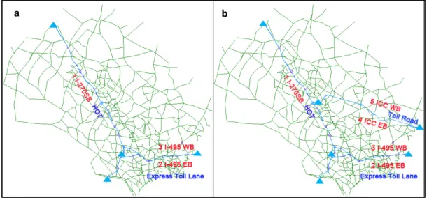
Fig. 1. Simulation network and toll road locations. (a) Base Year 2010; (b) Future Year 2030.
As shown in Fig. 1, this simulation road network covers the central and eastern Montgomery County and northwestern Prince George's County in Maryland. It includes all freeways, most major/minor arterials, and some local connectors/streets. Three major freeways: I-270, North I-495 and MD 200 (Inter-County Connector, ICC) are located in the middle of this study area. The network contains 449 traffic analysis zones, 5,480 links (totally 2,606.25
miles in length) and 1,978 nodes. There are 789 intersections directly cut from the traffic demand model of the Metropolitan Washington Council of Governments and imported into DTALite. In our case study, 268 pre-timed signals are coded into DTALite for all intersections that have signals in real world. Four modes of dynamic Origin-Destination (OD) matrices, i.e. SOV, HOV-2, HOV-3+, and trucks, were estimated based on the regional planning model and calibrated using field traffic counts data of 160 fixed sensors.
In Table 1, three scenarios are conducted for the morning peak period (6:00 AM to 9:00 AM), i.e. the base year (2010) without tolls (baseline), base year with tolls and future year (2030) with tolls. There are no pricing facilities in the baseline network. Since this case study aims to jointly optimize different types of road pricing strategies for a large-scale network, two optimal toll scenarios of the base year and the future year are designed for a comparison with the baseline. In the scenario of base year with tolls, specifically, we assume that an HOT lane is implemented on I-270 SB by the conversion of the existing inner HOV lane, and two extra express toll lanes are added to I-495 EB/WB, see Fig. 1(a). In addition to the base-year network, a new toll road (ICC) will be completed by 2015. ICC is implemented in the scenario of the future year with tolls, which is illustrated in Fig. 1(b).
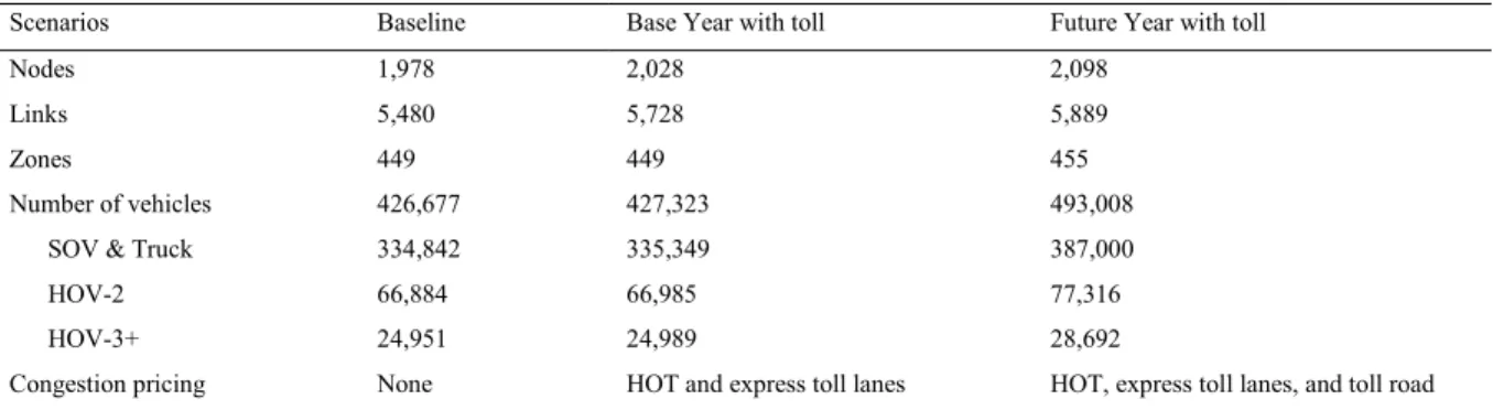
Table 1. Road networks and demand of three simulation scenarios.
Scenarios Baseline Base Year with toll Future Year with toll
Nodes 1,978 2,028 2,098
Links 5,480 5,728 5,889
Zones 449 449 455
Number of vehicles 426,677 427,323 493,008 SOV & Truck 334,842 335,349 387,000
HOV-2 66,884 66,985 77,316
HOV-3+ 24,951 24,989 28,692
Congestion pricing None HOT and express toll lanes HOT, express toll lanes, and toll road
3.2.Toll facilities
The objectives of the network congestion pricing problem include minimizing the average travel time for all finished trips and maximizing toll revenue during the 3-hour morning peak period. The decision variables are distanced-based toll rates of the HOT lane, express toll lanes, and the toll road. As shown in Table 1,
x
1 is the distance-based HOT toll rate of I-270 SB;x
2 andx
3 are distance-based rates on express toll lanes of I-495 EB and I-495 WB, respectively. Those three-dimensional decision variables are for the base-year scenario. In addition, we have five-dimensional decision variables for the future-year scenario, wherex
4 andx
5 are distance-based toll rates of the full toll road of ICC EB and WB, respectively. As shown in Table 2, the box constraints are xmin and xmax, which are thelower and upper boundaries, respectively.
Table 2. Toll facilities and decision variables.
Toll type Toll facilities Free access Decision variables Lower bound (US$/mile) Upper bound (US$/mile) Length (mile) Toll lane(s) Total lanes HOT I-270 SB HOV-2+ x1 0 0.50 23.04 1 6
Express toll lanes I-495 EB HOV-3+ x2 0 0.50 14.90 2 6
Express toll lanes I-495 WB HOV-3+ x3 0 0.50 14.30 2 6
Toll road ICC EB No free x4 0 0.50 15.42 3 3
Toll road ICC WB No free x5 0 0.50 15.43 3 3
We will briefly introduce the three major freeway corridors in these networks as follows.
Interstate 270 (I-270) is a 23.04-mile auxiliary Interstate Highway that travels between Gaithersburg, Rockville, and I-495 (the Capital Beltway) just north of Bethesda. It consists of a 20.94-mile mainline as well as a 2.10-mile spur
that provides access to and from southbound I-495. This portion of I-270 is up to twelve lanes wide and consists of a local-express lane configuration as well as HOV lanes that are in operation during peak travel times. I-270 heads southeast to an interchange with I-495 and MD 355 in suburban Bethesda, Montgomery County as a six-lane freeway with a 55 mph speed limit. The left lane on northbound is operated as a HOV lane between 3:30 and 6:30 PM weekdays and the same thing happens between 6:00 and 9:00 AM weekdays on southbound. In the simulation network, we assume I-270 SB utilizes the left lane as a HOT lane in the morning peak.
North Interstate 495 (I-495) is a 14.60-mile Interstate Highway that surrounds the north Washington, D.C., and the city's inner suburbs in adjacent Maryland. The Beltway passes through Prince George's County and Montgomery County in Maryland in the study area. We assume the express toll lanes to be a predictable option on the North I-495. Actually, they are already in operation on the Virginia side of the I-495. The express toll lanes operate alongside existing highway lanes to provide users with a faster and more predictable travel option. Carpools (HOV-3+), transit vehicles, motorcycles and emergency vehicles have free access to the express toll lanes. Drivers with fewer than three occupants shall pay to access. There are multiple entry and exit points to and from the express toll lanes.
The ICC lies at the north of the Capital Beltway and links several major north-south direction corridors in this area. It is a six-lane, toll highway that connects I-270 at I-370 in eastern Montgomery County to I-95 in northwestern
Prince George’s County. The construction of ICC is supposed to serve the traffic between the Montgomery County and the Prince Georges’ County, and alleviate the congestion on I-495 by diverting part of the traffic between the two counties. The ICC is an all-electronic toll facility that charges vehicles with E-ZPass directly when they travel through. The first segment of the ICC from I-370 at Shady Grove to MD 97 in Rockville/Olney opened in early 2011. The second segment from MD 97 to I-95 at Laurel opened in November 2011. In the simulation network, we assume the ICC EB/WB will be tolled for six lanes in both directions, while the peak distance-based toll rate is to be optimized.
4.Results and comparison
4.1.Simulation results
Applying the Latin hypercube sampling technique, we independently generate 100 sample vectors for the three-dimensional optimization problem of the base-year scenario, and 200 sample vectors for the five-three-dimensional optimization problem of the future-year scenario, respectively. As the cases of the minimum toll (zero toll; travelers with free access to toll roads), maximum toll are of interest to us, they’re also incorporated into the initial samples. For a comparison purpose, the baseline scenario (no implementation of any road pricing strategies) is also evaluated via simulation. Through our observation, the simulation noise generated by DTALite can be negligible in this study, in other words, the simulation results are stable if we run repetitions of the same road pricing strategy. For each evaluation of the initial samples, the DTA was conducted iteratively until convergence was achieved. We set the number of iteration to be 20, and found the percentage of travelers who switched routes was below 1.67% for all the experiments. Thus, we verify that for each simulation run, convergence is achieved after assignments and vehicular platoon simulations, and thus the simulator obtains valid results.
The average travel time is estimated by DTALite based on the experienced travel time of vehicles that finished their trips for every minute. On a 2-core, 24-CPU, 84-GB memory workstation, it takes around 20 minutes to finish a 20-iteration mesoscopic DTA for the Montgomery County network. Statistics of the initial sample and infill strategies are shown in Table 3 and Table 4, respectively.
4.2.Scenarios comparison
As the simulation of the Montgomery County network costs about 20 minutes for each network road pricing strategy, the surrogate models help reduce tremendous computation time compared to meta-heuristics that intensively recall objective evaluations, as well as traditional gradient-based methods that need to know the explicit form of the objective function. At the end of infill vectors (i.e. the 50th objective function evaluation for the base year, the 100th objective function evaluation for the future year), the best solutions are
* 2010
I-270 SB I-495 EB I-495 WB [HOT] [Express toll lanes] [Express toll lanes]
T [ ˆ 0.3041, 0.4978 , 0.3981 ] US$/mile x * 2030
I-270 SB I-495 EB I-495 WB ICC EB ICC WB
[HOT] [Express toll lanes] [Express toll lanes] [Toll road] [Toll T
road]
ˆ [0.4915, 0.3219 , 0.4998 , 0.4396 ,0.2106] US$/mile
x
The detailed comparison of the three scenarios are shown in Table 5. We then use both solutions as the simulation inputs. The best solution for the base year produces the network average travel time *
TT(ˆ2010) 16.20
f x min, which is
much smaller than the baseline f(xbaseline) 20.05 min. The base year optimal toll revenue is US$2,407.35, which is
of course more than the baseline of zero revenue. The best solution for the future year shows that the network average travel time is *
TT(ˆ2030) 23.30
f x min, and the toll revenue is US$32,250.56.
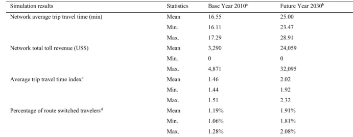
Table 3. Statistics of simulation results for initial design of experiments.
Simulation results Statistics Base Year 2010a Future Year 2030b
Network average trip travel time (min) Mean 16.55 25.00 Min. 16.11 23.47 Max. 17.29 28.91 Network total toll revenue (US$) Mean 3,290 24,059
Min. 0 0
Max. 4,871 32,095 Average trip travel time indexc Mean 1.46 2.02
Min. 1.44 1.92 Max. 1.51 2.32 Percentage of route switched travelersd Mean 1.19% 1.91%
Min. 1.06% 1.81% Max. 1.28% 2.08%
a The number of initial vectors in the base year is 100; b The number of initial vectors in the future year is 200; c Trip travel time index is the trip
travel time divided by free flow travel time; d At the end of 20 iterations of DTA, the percentage of switched routes of all travelers.
Table 4. Statistics of simulation results for infill vectors.
Simulation results Statistics Base Year 2010a Future Year 2030b
Network average trip travel time (min) Mean 16.54 25.00 Min. 16.17 23.47 Max. 17.16 28.91 Network total toll revenue (US$) Mean 3,504 28,595
Min. 1,239 13,213 Max. 4,829 33,377 Average trip travel time index Mean 1.46 1.99
Min. 1.44 1.92 Max. 1.51 2.21 Percentage of route switched travelers Mean 1.18% 1.92%
Min. 1.07% 1.74% Max. 1.29% 2.08%
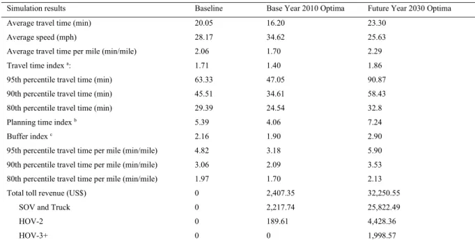
Table 5. Simulation results of the baseline and optimal solutions.
Simulation results Baseline Base Year 2010 Optima Future Year 2030 Optima Average travel time (min) 20.05 16.20 23.30
Average speed (mph) 28.17 34.62 25.63 Average travel time per mile (min/mile) 2.06 1.70 2.29 Travel time index a: 1.71 1.40 1.86
95th percentile travel time (min) 63.33 47.05 90.87 90th percentile travel time (min) 45.51 34.61 58.43 80th percentile travel time (min) 29.39 24.54 32.8 Planning time index b 5.39 4.06 7.24
Buffer index c 2.16 1.90 2.90
95th percentile travel time per mile (min/mile) 4.82 3.18 5.90 90th percentile travel time per mile (min/mile) 3.06 2.09 3.53 80th percentile travel time per mile (min/mile) 1.97 1.70 2.13 Total toll revenue (US$) 0 2,407.35 32,250.55
SOV and Truck 0 2,217.74 25,822.49
HOV-2 0 189.61 4,428.36
HOV-3+ 0 0 1,998.57
a Average travel time divided by free-flow travel time; b The 95th percentile travel time divided by free-flow travel time; c (The 95th percentile
travel time – average travel time) divided by average travel time.
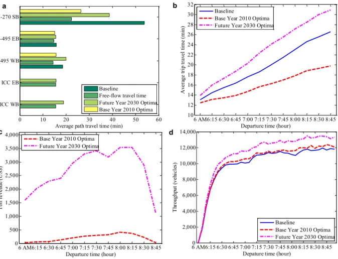
Fig. 2(a) compares the average experienced travel time of the toll facilities between the baseline and two optimal road pricing scenarios. The major performance improvement is on the freeway I-270 SB. The optimal result of the base year shows a significant reduction in travel time compared with the baseline in which no road pricing strategies or additional lanes are implemented. Though the future-year network-wide demand increases by 16%, travel time along I-270 SB is still much shorter than the baseline. Both directions of I-495 are improved as their path travel times slightly decrease in the base-year optimal pricing compared with the baseline. It is worthy to note that we compare path travel times on the general-purpose lanes of I-270 and I-495, because the capacities of the HOT lane or express
toll lanes are not fully utilized. Thus path travel time on toll managed lanes doesn’t change significantly due to the
toll. While for ICC, we compare its travel time with the free-flow travel time for the future year.
As the network average travel time fluctuates significantly at the one-minute interval, Fig. 2(b) illustrates the average travel time in 15-min interval for the entire network. It clearly shows that the network average travel time is reduced in the base-year optimal case compared to the baseline. It again verifies that the SBO solution significantly improves the network performance on congestion mitigation. In the last hour of the morning peak which is the most congested period, there are the most vehicles and the longest travel time in the study network. Thus the optimal design strategy successfully helps alleviate congestion. Furthermore, we can predict effects of the optimal road pricing strategy on the network for the future year. It is regular to see that the network becomes more congested because more demand is loaded, but the predicted travel time profile can be regarded as the benchmark for the future year traffic analysis.
Various other network wide performance measures are also compared between different scenarios. The toll revenue and vehicle throughput are illustrated in Fig. 2(c-d). In the future-year scenario, due to the significant increase of users in the network, toll revenue collected during the morning peak period is significantly higher than the base-year optima scenario. The overall increase of the toll revenue for the optimal toll case than the base-year optima during the three-hour peak period is about US$29,843. Moreover, when we compare the base-year optima and the baseline, the improvement in travel time brings in additional benefits. The throughput for the whole network increases significantly from 7:45 to 9:00 am, and the total throughput for the morning peak period increased by about 2.83% under the optimal road pricing. The adjustment of toll rates of three types of pricing policies in the large-scale network has successfully led to a more efficient usage of the road network capacity.
Fig. 2. Comparison of baseline and optima. (a) Average path travel time of toll facilities; (b) network-wide average trip travel time; (c) time-varying toll revenue; (d) network-wide time-time-varying throughput.
Overall, the optimal road pricing to the network supply improvement in the base year induces a 19.20% reduction in the average travel time of all users during the morning peak. The monetary savings are about US$408.12 thousands if we multiply the total saving time by the mean value of time (US$15/hour) for the 3-hour simulation. If we consider every hour of each day, and even consider over an entire year, such a combined network road pricing strategy would mean a huge saving from an operational and policy standpoint. Thus the optimal solution given by the surrogate model should be an encouraging policy option to enhance transportation system performance in the study areas.
In addition to the various time-varying network performance measures aforementioned, we explore the distributions of hundreds of thousands of individual travel time and travel distance, see Fig. 3. The travel time cumulative distribution shows the improvement of the base-year optima compared to the baseline, while the increase of travel time for the future year is inevitable, however, we show a benchmark of the optimal road pricing for the
future demand. The travel distance doesn’t change much because most travelers makes choices between toll lanes and
general-purpose lanes. Thus the travel distance cumulative distribution of the baseline is almost the same as the base-year optima. Fig. 3(b) omits the cumulative distribution of the baseline.
0 10 20 30 40 50 60 ICC WB ICC EB I-495 WB I-495 EB I-270 SB
Average path travel time (min) Baseline
Free-flow travel time Future Year 2030 Optima Base Year 2010 Optima
6 AM6:15 6:30 6:45 7:00 7:15 7:30 7:45 8:00 8:15 8:30 8:45 10 12 14 16 18 20 22 24 26 28 30 32
Departure time (hour)
A ve ra ge tr ip tra ve l t ime (mi n) Baseline
Base Year 2010 Optima Future Year 2030 Optima
6 AM6:15 6:30 6:45 7:00 7:15 7:30 7:45 8:00 8:15 8:30 8:45 0 500 1,000 1,500 2,000 2,500 3,000 3,500 4,000
Departure time (hour)
T oll r ev en ue (U S$ )
Base Year 2010 Optima Future Year 2030 Optima
6 AM6:15 6:30 6:45 7:00 7:15 7:30 7:45 8:00 8:15 8:30 8:450 2,000 4,000 6,000 8,000 10,000 12,000 14,000
Depature time (hour)
T hr ou ghp ut (ve hi cl es ) Baseline
Base Year 2010 Optima Future Year 2030 Optima
a b
d c
Fig. 3. (a) Cumulative distributions of trip travel time; (b) cumulative distributions of trip travel distance.
5.Conclusions
This paper builds a SBO framework and tests it with a real-world application. The basic idea of SBO is to construct a surrogate model to approximate the true objective function, and use the surrogate to search for optimal solutions. As the real optimization process is based on the surrogate model, a large number of function evaluations through simulations can be saved. The total computation time for the optimization is thus significantly reduced.
Applying the proposed SBO method to a real-world network with three types of toll facilities in Maryland, i.e. HOT lanes, express toll lanes, and toll roads, we optimize distance-based toll rates to jointly minimize the network wide average travel time and maximize the toll revenue. Three representative scenarios are selected to demonstrate the feasibility of surrogate models in solving the network road pricing problem in a large-scale network with multiple types of toll facilities, i.e. the baseline without toll facilities, optimal pricing for the base year (2010), and optimal pricing for the future year (2030). Overall, the simulation results show that implementing the optimal road pricing strategy predicted by the surrogate model benefits travelers in saving their average travel time to a remarkable extent and generates toll revenue for decision-makers. We find that the SBO with infill by expected improvement for the base year obtains a 19.20% reduction in the average travel time compared with the baseline, and generates US$2,407 on priced managed lanes during the morning peak. The toll revenue is even higher for the future year when the toll road ICC is open.
In the future, one research question we’d like to investigate is whether the willingness to pay of travelers for the priced managed lanes and toll roads impacts the network simulation results. Quantitative studies can be conducted by using field data such as stated preference surveys. Another research issue is the behavioral assumption in this paper is dynamic route choice, i.e. DUE, however, travelers have more dimensions of choice behavior that may influence the simulation outputs and thus the SBO results. Not every traveler stops searching the dynamic shortest route until the DUE conditions are satisfied, but in fact, travelers may stop searching routes halfway from the agent-based modeling perspective, which may accelerate simulation convergence as well as enhance the behavior realism. DUE can be replaced by behavioral user equilibrium in terms of departure time choice, en-route choice, mode choice, etc.
Acknowledgements
This research is financially supported by a National Science Foundation CAREER Award “Reliability as an Emergent Property of Transportation Networks”, and the U.S. Federal Highway Administration.
0 20 40 60 80 100 120 140 160 180 0 0.5 1 1.5 2 2.5 3 3.5 4 4.5 5x 10 5
Travel time (min)
C umu la tiv e v eh ic le s Baseline
Base Year 2010 Optima Future Year 2030 Optima
0 10 20 30 40 50 0 0.5 1 1.5 2 2.5 3 3.5 4 4.5 5x 10 5
Travel distance (mile)
C umu la tiv e v eh ic le s
Base Year 2010 Optima Future Year 2030 Optima
References
Barton, R. R., Meckesheimer, M., 2006. Metamodel-based simulation optimization. Handbooks in Operations Research and Management Science 13, 535-574.
Chen, X., Zhang, L., He, X., Xiong, C., Li, Z., 2014a. Surrogate-based optimization of expensive-to-evaluate objective for optimal highway toll charges in transportation network. Computer-Aided Civil and Infrastructure Engineering 29(5), 359-381.
Chen, X., Yin, M., Song, M., Zhang, L., Li M., 2014b. Social welfare maximization of multimodal urban transportation systems using metamodel: A simulation study of Tianjin Eco-City in China. Transportation Research Record, in press.
Chen, X., Xiong, C., He, X., Zhu, Z., Zhang, L., 2015a. Congestion pricing for improving network service: A simulation-based optimization approach, 94th Annual Meeting of Transportation Research Board. Washington, DC.
Chen, X., He, X., Xiong, C., Zhang, L., 2015b. A Bayesian stochastic Kriging metamodel for simultaneous optimization of travel behavioral responses and traffic management, 94th Annual Meeting of Transportation Research Board. Washington, DC.
Chen, X., Zhu, Z., He, X., Zhang, L.*, 2015c. Surrogate-based optimization for solving mixed integer network design problem, 94th Annual Meeting of Transportation Research Board. Washington, DC.
FHWA, 2006. Congestion Pricing: A Primer. Federal Highway Administration, Washington D.C.
Forrester, A., Sobester, A., Keane, A., 2008. Engineering Design via Surrogate Modelling: A Practical Guide. John Wiley & Sons. Fu, M., 2002. Optimization for simulation: Theory vs. practice. INFORMS Journal on Computing 14(3), 192-215.
He, X., Chen, X., Xiong, C., Zhu, Z., Zhang, L., 2015. Integrated optimization of transportation demand management and traffic operations using simulation: A bootstrapped support vector regression method considering the statistical distribution of simulation noise, 94th Annual Meeting of Transportation Research Board. Washington, DC.
He, X., Chen, X., Xiong, C., Zhang, L.*, 2013. Simulation-based optimization for highway toll charge using surrogate modelling, Conference on Agent-Based Modeling in Transportation Planning and Operations. Blacksburg, Virginia.
Hearn, D. W., Ramana, M. V., 1998. Solving congestion toll pricing models, in “Equilibrium and Advanced Transportation Modeling”. In: Marcotte,
P., Nguyen, S. (Ed.). Kluwer Academic Publishers, pp. 109-124.
Huang, D., Allen, T. T., Notz, W. I., Zeng, N., 2006. Global optimization of stochastic black-box systems via sequential Kriging meta-models. Journal of Global Optimization 34(3), 441-466.
Lu, C.-C., Mahmassani, H. S., Zhou, X., 2008. A bi-criterion dynamic user equilibrium traffic assignment model and solution algorithm for evaluating dynamic road pricing strategies. Transportation Research Part C 16(4), 371-389.
Montgomery, D. C., 2008. Design and Analysis of Experiments. John Wiley & Sons.
Perez, B. G., Fuhs, C., Gants, C., Giordano, R., Ungemah, D. H., 2012. Priced Managed Lane Guide. No. FHWA-HOP-13-007.
Shepherd, S., Sumalee, A., 2004. A genetic algorithm based approach to optimal toll level and locations problems. Network and Spatial Economics 2(4), 161-179.
Song, M., Yin, M., Chen, X., Zhang, L., Li, M., 2013. A simulation-based approach for sustainable transportation systems evaluation and optimization: Theory, systematic framework and applications, 13th COTA International Conference of Transportation Professionals. Shenzhen, China.
Verhoef, E. T., 1996. The Economics of Regulating Road Transport. Cheltenham, U.K.
Verhoef, E. T., 2002. Second-best congestion pricing in general static transportation networks with elastic demand. Regional Science and Urban Economics 32(3), 281-310.
Xiong, C., Zhu, Z., He, X., Chen, X., Zhu, S., Mahapatra, S., Chang, G., Zhang, L., 2015. Developing a 24-Hour Large-Scale Microscopic Traffic Simulation Model for the Before-and-After Study of a New Tolled Freeway in the Washington, DC–Baltimore Region. ASCE Journal of Transportation Engineering DOI. 10.1061/(ASCE)TE.1943-5436.0000767, 05015001.
Yang, H., Huang, H. J., 1999. Carpooling and congestion pricing in a multilane highway with high-occupancy-vehicle lanes. Transportation Research Part A 33(2), 139-155.
Yang, H., Lam, W., 1996. Optimal road tolls under conditions of queuing and congestion. Transportation Research Part A 30(5), 319-332.
Yang, H., Zhang, X. N., 2002. Determination of optimal toll levels and toll locations of alternative congestion pricing schemes, in “Proceedings of
the 15th International Symposium in Transportation and Traffic Theory”. In: Taylor, M. A. P. (Ed.), Pergamon, 519-540.
Yin, Y., 2002. Multiobjective bilevel optimization for transportation planning and management problems. Journal of Advanced Transportation 36(1), 93-105.
Zhang, L., Chen, X., He, X., Xiong, C., 2014. Bayesian stochastic Kriging metamodel for active traffic management of corridors, 2014 Industrial and Systems Engineering Research Conference and Expo. Montreal, Canada.