A Practical Model for Subsurface Light Transport
Henrik Wann Jensen
Stephen R. Marschner
Marc Levoy
Pat Hanrahan
Stanford University
Abstract
This paper introduces a simple model for subsurface light transport in translucent materials. The model enables efficient simulation of effects that BRDF models cannot capture, such as color bleeding within materials and diffusion of light across shadow boundaries. The technique is efficient even for anisotropic, highly scattering media that are expensive to simulate using existing methods. The model combines an exact solution for single scattering with a dipole point source diffusion approximation for multiple scattering. We also have designed a new, rapid image-based measurement tech-nique for determining the optical properties of translucent materi-als. We validate the model by comparing predicted and measured values and show how the technique can be used to recover the opti-cal properties of a variety of materials, including milk, marble, and skin. Finally, we describe sampling techniques that allow the model to be used within a conventional ray tracer.
Keywords: Subsurface scattering, BSSRDF, reflection models, light transport, diffusion theory, realistic image synthesis
1
Introduction
Accurately modeling the scattering of light by materials is funda-mental for realistic image synthesis. Even the most sophisticated light transport algorithms fail to produce convincing results if the local scattering models are too simple. Therefore a great deal of research has gone into describing the scattering of light from mate-rials.
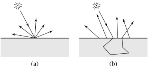
Previous research has focused on developing models for the bidirectional reflectance distribution function (BRDF). The BRDF was introduced by Nicodemus [14] as a simplification of the more general bidirectional surface scattering distribution function (BSSRDF). The BSSRDF can describe light transport between any two rays that hit a surface, whereas the BRDF assumes that light en-tering a material leaves the material at the same position (Figure 1). This approximation is valid for metals, but it fails for translucent materials, which exhibit significant transport below the surface. Even for many materials that do not seem very translucent, using the BRDF creates a hard, distinctly computer-generated appearance because it does not locally blend surface features such as color and geometry. Only methods that consider subsurface scattering can capture the true appearance of translucent materials, such as mar-ble, cloth, paper, skin, milk, cheese, bread, meat, fruits, plants, fish, ocean water, snow, etc.
1.1 Previous Work
Almost all BRDF models are derived exclusively from surface scat-tering, with any subsurface scattering approximated by a Lam-bertian component. An exception is the model by Hanrahan and Krueger [10] which includes an analytic expression for single scat-tering in a homogeneous, uniformly lit slab. However, all BRDF models ultimately assume that light scatters at one surface point and they do not model subsurface transport from one point to another.
Subsurface transport can be simulated accurately but slowly by solving the full radiative transfer equation [1]. Only a few papers in graphics have taken this approach to subsurface scattering. Dorsey et al. [5] simulated full subsurface scattering using photon mapping to capture the appearance of weathering in stone. Pharr and Han-rahan [15] used scattering functions to simulate subsurface scat-tering. These approaches, while capable of simulating all of the effects of subsurface scattering, are computationally very expen-sive compared to the simulation of opaque materials. Techniques based on path sampling are particularly inefficient for highly scat-tering materials, such as milk and skin, in which light scatters mul-tiple (often several hundred) times before exiting the material. For highly scattering media Stam [17] introduced the use of diffusion theory. He solved a diffusion equation approximation using a multi-grid method, and used this method to render clouds with multiple scattering.
Subsurface scattering is also important in medical physics, where models have been developed to describe the scattering of laser light in human tissue [6, 8]. In that context, diffusion theory is often used to predict as well as to measure the optical properties of highly scat-tering materials. We have extended this theory for use in computer graphics by adding exact single scattering, support for arbitrary ge-ometry, and a practical sampling technique for rendering.
In measurements of appearance for computer graphics, subsur-face scattering has rarely been considered. Debevec et al. [3] mea-sured light reflection from human faces, which included contribu-tions from subsurface scattering, but they did not relate the data to the physical properties of the material. Again building on medical physics research [8, 9], we have extended a methodology developed for measuring biological tissues into a rapid image-based appear-ance measurement technique for translucent materials. This method examines the radial reflectance profile resulting from a beam illu-minating the sample material. By fitting an expression derived from diffusion theory it is possible to estimate the absorption and scatter-ing properties of the material.
2
Theory
The BSSRDF,S, relates the outgoing radiance,Lo(xo, ~ωo)at the pointxoin direction~ωo, to the incident flux,Φi(xi, ~ωi)at the point
xifrom direction~ωi[14]:
dLo(xo, ~ωo) =S(xi, ~ωi;xo, ~ωo)dΦi(xi, ~ωi).
The BRDF is an approximation of the BSSRDF for which it is assumed that light enters and leaves at the same point (i.e.,
(a) (b)
Figure 1: Scattering of light in (a) a BRDF, and (b) a BSSRDF.
by integrating the incident radiance over incoming directions and area,A: Lo(xo, ~ωo) = Z A Z 2π S(xi, ~ωi;xo, ~ωo)Li(xi, ~ωi) (~n·~ωi)dωidA(xi). Light propagation in a participating medium is described by the radiative transport equation, often referred to in computer graphics as the volume rendering equation:
(~ω·∇~)L(x, ~ω) =−σtL(x, ~ω)+σs Z
4π
p(~ω, ~ω0)L(x, ~ω0)dω0+Q(x, ~ω).
In this equation, the properties of the medium are described by the absorption coefficientσa, the scattering coefficientσs, and the phase functionp(~ω, ~ω0). The extinction coefficientσt is defined as,σt =σa+σs. We assume the phase function is normalized, R
4πp(~ω, ~ω
0)dω0 = 1and is a function only of the phase angle, p(~ω, ~ω0) =p(~ω·~ω0). The mean cosine,g, of the scattering angle is
g=
Z
4π
(~ω·~ω0)p(~ω·~ω0)dω0.
Ifgis positive, the phase function is predominantly forward scat-tering; ifgis negative, backward scattering dominates. A constant phase function results in isotropic scattering (g= 0).
For an infinitesimal beam entering a homogeneous medium, the incoming radiance will decrease exponentially with distances. This is referred to as the reduced intensity:
Lri(xi+s~ωi, ~ωi) =e−σtsLi(xi, ~ωi).
The first-order scattering of the reduced intensity, Lri, may be treated as a volumetric source:
Q(x, ~ω) =σs Z
4π
p(~ω0, ~ω)Lri(x, ~ω0)dω0.
To gain insight into the volumetric behavior of light propaga-tion, it is useful to integrate the radiative transport equation over all directions~ωat a pointxwhich yields
~
∇ ·E~(x) =−σaφ(x) +Q0(x). (1)
This equation relates the scalar irradiance, or fluence,
φ(x) = R
4πL(x, ~ω)dω, and the vector irradiance,
~
E(x) = R4πL(x, ~ω)~ω dω. In the absence of loss due to ab-sorption or gain due to a volumetric light source(Q0 = 0), the
divergence of the vector irradiance equals zero. In this equation, we introduce a 0th-order source term,Q0, and later we will need
the 1st-order source term,Q~1, where
Q0(x) = Z 4π Q(x, ~ω)dω, Q~1(x) = Z 4π Q(x, ~ω)~ω dω. S BSSRDF Rd Diffuse BSSRDF Fr Fresnel reflectance Ft Fresnel transmittance
Fdr Diffuse Fresnel reflectance
~ E Vector irradiance φ Radiant fluence σa Absorption coefficient σs Scattering coefficient σt Extinction coefficient
σt0 Reduced extinction coefficient
σtr Effective extinction coefficient
D Diffusion constant
α Albedo
p Phase function
η Relative index of refraction
g Mean cosine of the scattering angle
Q Volume source distribution
Q0 0th-order source distribution
~
Q1 1st-order source distribution Figure 2: Selected symbols.
2.1 The Diffusion Approximation
The diffusion approximation is based on the observation that the light distribution in highly scattering media tends to become isotropic. This is true even if the initial light source distribution and the phase function are highly anisotropic. Each scattering event blurs the light distribution, and as a result the light distribution tends toward uniformity as the number of scattering events increases.
In this situation, the radiance may be approximated by a two-term expansion involving the radiant fluence and the vector irradi-ance:
L(x, ~ω) = 1 4πφ(x) +
3
4π~ω·E~(x).
The constants are determined by the definitions of fluence and vec-tor irradiance.
The diffusion equation follows from this approximation. Specif-ically, we substitute this two-term expansion of the radiance into the radiative transport equation and then integrate over~ω; for the algebraic details consult Ishimaru [12]. The result is
~
∇φ(x) =−3σ0tE~(x) +Q~1(x). (2)
Here we have used the reduced extinction coefficient,σt0, which is given by
σt0=σ0s+σa where σs0 =σs(1−g).
The reduced scattering coefficientσ0sscales the original scattering coefficient by a factor of(1−g). Intuitively, once light becomes isotropic, only backward scattering terms change the net flux; for-ward scattering is indistinguishable from no scattering.
In the case where there are no sources, or where the sources are isotropic,Q~1vanishes from Equation 2. Then the vector irradiance
is the gradient of the scalar fluence,
~
E(x) =−D ~∇φ(x).
HereD= 1 3σ0
t
is the diffusion constant. This equation makes pre-cise the intuitive notion that there is net energy flow (i.e., non-zero vector irradiance) from regions of high energy density (high flu-ence) to regions of low energy density.
Finally, substituting Equation 2 into Equation 1, we arrive at the classic diffusion equation
The diffusion equation has a simple solution in the case of a sin-gle isotropic point light source in an infinite medium.
φ(x) = Φ 4π D
e−σtrr(x)
r(x) ,
whereΦis the power of the point light source,ris the distance to the location of the point source, andσtr =
p
3σaσ0tis the effective transport coefficient. The point source results in an energy density in the volume with an exponential falloff.
In the case of a scattering medium in a finite region of space, the diffusion equation must be solved subject to the appropriate bound-ary conditions. The boundbound-ary condition is that the net inward dif-fuse flux is zero at each point,xs, on the surface
Z
2π−
L(xs, ~ω)(~ω·~n(xs))dω= 0.
Here,2π−denotes integration over the hemisphere of inward di-rections. Using the two-term expansion, the boundary condition is
φ(xs)−2D(~n·∇~)φ(xs) = 0. (3) The minus sign in the second term results from the convention that the surface normal points outward, whereas the integral is over in-ward directions.
Equation 3 covers the case where the two layers have matching indices of refraction, but another important case is where these in-dices differ. When an interface exists between media with different refractive indices, there is a reflection at the interface. AssumingFr is the Fresnel formula for the reflectance at a dielectric interface, the average diffuse Fresnel reflectance is
Fdr= Z
2π
Fr(η, ~n·~ω0)(~n·~ω0)dω0,
whereηis the relative index of refraction of the medium with the reflected ray to the other medium. Fdrmay be computed analyti-cally from the Fresnel formula [13]. However, we will use a rational approximation of the measured diffuse reflectance [7]:
Fdr=−
1.440 η2 +
0.710
η + 0.668 + 0.0636η.
The resulting boundary condition between two media with different indices of refraction is Z 2π− L(x, ~ω)(~ω·~n−)dω=Fdr Z 2π+ L(x, ~ω)(~ω·~n+)dω.
Here the+and−subscript means outward and inward directions respectively. This yields
φ(xs)−2D(~n·∇~)φ(xs) =Fdr
φ(xs) + 2D(~n·∇~)φ(xs)
.
Note that the difference in signs between the two sides of this equa-tion occurs because one integral is over outward direcequa-tions and the other is over inward directions. Rearranging terms,
φ(xs)−2AD(~n·∇~)φ(xs) = 0.
This boundary condition is the same as when the indices of refrac-tion match (Equarefrac-tion 3); the only difference is that2Dis replaced by2AD, where
A=1 +Fdr 1−Fdr
.
Finally, the boundary condition allows us to compute the diffuse BSSRDF,Rd. Rd is equal to the radiant exitance divided by the incident flux. The radiant exitance leaving the surface(~n·E~(xs))
is equal to the gradient of the fluence at the surface
Rd(r) =−D
(~n·∇~φ)(xs)
dΦi(xi)
,
wherer=||xs−xi||.
In the case of finite media, the diffusion equation does not in general have an analytical solution. In this paper we are interested in subsurface reflection, which is often modeled as a semi-infinite parallel medium. Several authors have analyzed the plane-parallel problem for simple source geometries, in particular, ap-proximations of a cylindrical beam entering the media. Exact for-mulas exist, but they involve an infinite sum of Bessel functions [9, 16]. We seek a simple formula suitable for modeling subsurface reflection that does not involve infinite sums or numerical solution of a partial differential equation.
Eason [6] and Farrell et al. [8] have developed a method for approximating the volumetric source distribution using two point sources; that is, a dipole. Eason introduced this idea and derived explicit formulae for the dipoles for various source geometries, such as a cylindrical beam, by expanding the source distributions in terms of their moments. Farrell et al. proposed using a single dipole to represent the incident source distribution. They found a single dipole to be as accurate as, or, in some cases, more accurate than using the diffusion approximation with the true source distri-bution.
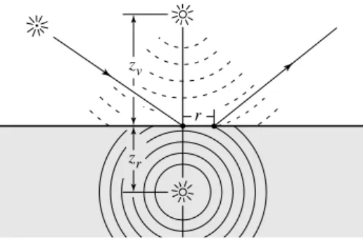
The dipole method consists of positioning two point sources near the surface in such a way as to satisfy the required boundary con-dition [6] (see Figure 3). One point source, the positive real light source, is located at the distancezr beneath the surface, and the other, the negative virtual light source, is located above the surface at a distancezv=zr+ 4AD. The resulting fluence is
φ(x) = Φ 4π D e−σtrdr dr − e−σtrdv dv ,
wheredr=||x−xr||is the distance fromxto the real source, and
dv =||x−xv||is the distance fromxto the virtual source. Far-rell et al. [8] proposed positioning the real light source at distance
zr = 1/σt, or one mean free path, below the surface. They only0 considered light parallel to the normal. For other light directions reciprocity can be enforced by still placing the light source1/σ0t straight belowxi.
The diffuse reflectance due to the dipole source can now be com-puted. Rd(r) =−D (~n·∇~φ(xs)) dΦi = α 0 4π (σtrdr+ 1) e−σtrdr σ0 td3r +zv(σtrdv+ 1) e−σtrdv σ0 td3v . (4) Lastly, we need to take into account the Fresnel reflection at the boundary for both the incoming light and the outgoing radiance.
Sd(xi, ~ωi;xo, ~ωo) =
1
πFt(η, ~ωi)Rd(||xi−xo||)Ft(η, ~ωo) (5)
whereSdis the diffusion term of the BSSRDF. This term represents multiple scattering (one scattering event is already included in the conversion to a point source). The next section explains how to compute the contribution due to single scattering.
zr zv
r
Figure 3: An incoming ray is transformed into a dipole source for the diffusion approximation.
2.2 Single Scattering Term
Hanrahan and Krueger [10] have derived a BRDF model for subsur-face reflection that analytically computes the total first-order scat-tering from a flat, uniformly lit, homogeneous slab. In this section, we show how their BRDF can be extended to a BSSRDF in order to account for local variations in lighting over the surface.
The total outgoing radiance, L(1)o , due to single scattering is computed by integrating the incident radiance along the refracted outgoing ray (see Figure 4):
L(1)o (xo, ~ωo) =σs(xo) Z 2π F p(~ω0i·~ωo0) Z ∞ 0 e−σtcsLi(xi, ~ωi)ds d~ωi (6) = Z A Z 2π S(1)(xi, ~ωi;xo, ~ωo)Li(xi, ~ωi) (~n·~ωi)dωidA(xi).
HereF = Ft(η, ~ωo)Ft(η, ~ωi)is the product of the two Fresnel transmission terms, and~ω0iand~ω0oare the refracted incoming and outgoing directions. The combined extinction coefficient σtc is given byσtc = σt(xo) +Gσt(xi), whereGis a geometry fac-tor; for a flat surfaceG= |~ni·~ω0o|
|~ni·~ω0i|. The single scattering BSSRDF, S(1)
, is defined implicitly by the second line of this equation. Note that there is a change of variables between the first line, which in-tegrates only over the configurations where the two refracted rays intersect, and the second line, which integrates over all incoming and outgoing rays. This implies that the distributionS(1)contains a delta function.
2.3 The BSSRDF Model
The complete BSSRDF model is a sum of the diffusion approxima-tion and the single scattering term:
S(xi, ~ωi;xo, ~ωo) =Sd(xi, ~ωi;xo, ~ωo) +S(1)(xi, ~ωi;xo, ~ωo) HereSdis evaluated using Equation 5 andS(1) is evaluated us-ing Equation 6. The parameters for the BSSRDF are: σa,σs,0 η, and possibly a phase function (without a phase function the scat-tering can be modeled as isotropic). This model accounts for light transport between different locations on the surface, and it simu-lates both the directional component (due to single scattering) as well as the diffuse component (due to multiple scattering).
Finally, note the distances involved in both the single scattering term and the diffusion approximations. The average exit point is approximately one mean free path from the entry point. However, these two mean free paths have quite different length scales. In the single scattering case, the mean free path equals1/σt; in the diffusion case, the mean free path equals1/σtr. For translucent materials whereσa σ0sand consequentlyσtr σt, the single scattering term decreases much faster than the diffusion term as the distance toxoincreases.
x s
i xo
Figure 4: Single scattering occurs only when the refracted incoming and outgoing rays intersect, and is computed as an integral over path lengthsalong the refracted outgoing ray.
2.4 BRDF Approximation
We can approximate the BSSRDF with a BRDF by assuming that the incident illumination is uniform. This assumption makes it pos-sible to integrate the BSSRDF over the surface. By integrating the diffusion term we find the total diffuse reflectanceRdof the mate-rial as: Rd= 2π Z ∞ 0 Rd(r)r dr= α0 2 1 +e−43A √ 3(1−α0) e− √ 3(1−α0) .
Notice how the diffuse reflectance only depends on the reduced albedo and the internal reflection parameterA.
The integration of the single scattering term results in the model presented in [10]. For a semi-infinite medium this gives:
fr(1)(x, ~ωi, ~ωo) =αF
p(~ωi0·~ω0o)
|~n·~ω0
i|+|~n·~ω0o|
.
The complete BRDF model is the sum of the diffuse reflectance scaled by the Fresnel term and the single scattering approximation:
fr(x, ~ωi, ~ωo) =fr(1)(x, ~ωi, ~ωo) +F
Rd
π .
This model has the same parameters as the BSSRDF. It is similar to the BRDF model presented in [10], but with the important differ-ence that the amount of diffusely reflected light is computed from the intrinsic material parameters. The BRDF approximation is use-ful for opaque materials, which have a very short mean free path.
3
Measuring the BSSRDF
To verify our BSSRDF model, and to determine appropriate pa-rameters for rendering different kinds of materials, we used the diffusion theory of Section 2 to make measurements of subsurface scattering in several media. Our measurement approach applies to translucent materials for whichσaσs, implying that far enough away from the point of illumination, we may neglect single scatter-ing and use the diffusion term to relate measurements to material parameters.
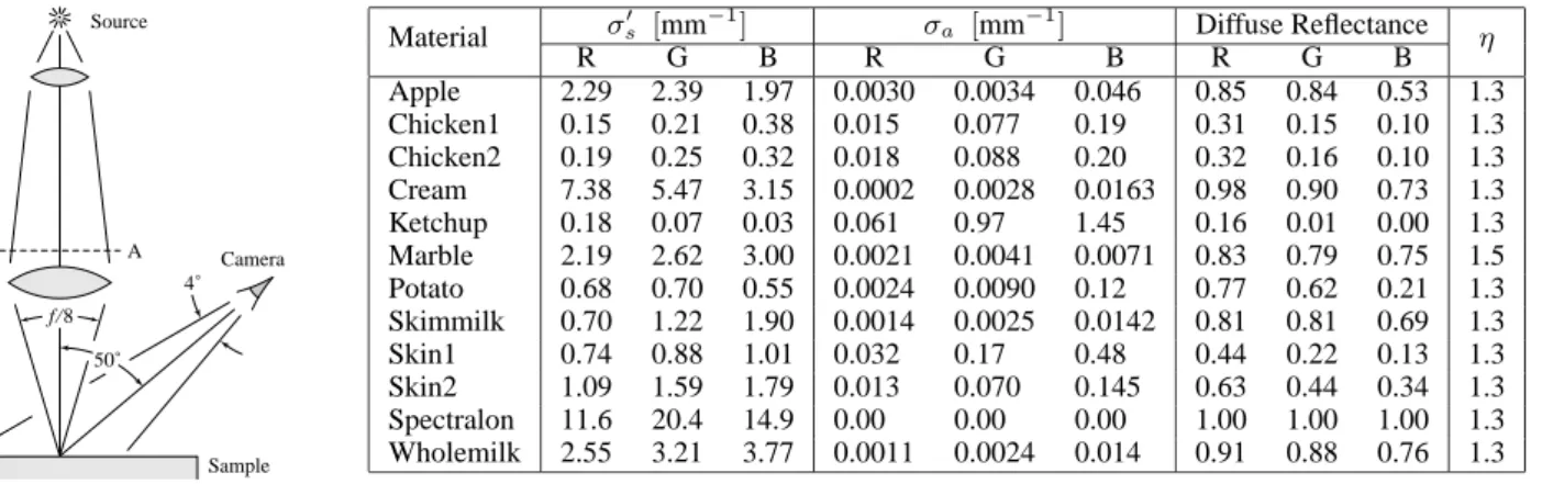
When multiple scattering dominates, Equation 4 predicts the ra-diant exitance per unit incident flux that will be observed due to a narrow incident beam, as a function of distance from the point of illumination. To make the corresponding measurement, we illumi-nate the surface of a sample with a tightly focused beam of white light and take a photograph using a 3-CCD video camera to observe the radiant exitance across the entire surface. We keep our obser-vations at constant angles so that the Fresnel term remains constant for all the measurements. Figure 5(a) illustrates our measurement setup.
50˚ 50mm 90cm A Camera Source Sample f/8 4 ˚ σs0 [mm−1] σa [mm−1] Diffuse Reflectance Material R G B R G B R G B η Apple 2.29 2.39 1.97 0.0030 0.0034 0.046 0.85 0.84 0.53 1.3 Chicken1 0.15 0.21 0.38 0.015 0.077 0.19 0.31 0.15 0.10 1.3 Chicken2 0.19 0.25 0.32 0.018 0.088 0.20 0.32 0.16 0.10 1.3 Cream 7.38 5.47 3.15 0.0002 0.0028 0.0163 0.98 0.90 0.73 1.3 Ketchup 0.18 0.07 0.03 0.061 0.97 1.45 0.16 0.01 0.00 1.3 Marble 2.19 2.62 3.00 0.0021 0.0041 0.0071 0.83 0.79 0.75 1.5 Potato 0.68 0.70 0.55 0.0024 0.0090 0.12 0.77 0.62 0.21 1.3 Skimmilk 0.70 1.22 1.90 0.0014 0.0025 0.0142 0.81 0.81 0.69 1.3 Skin1 0.74 0.88 1.01 0.032 0.17 0.48 0.44 0.22 0.13 1.3 Skin2 1.09 1.59 1.79 0.013 0.070 0.145 0.63 0.44 0.34 1.3 Spectralon 11.6 20.4 14.9 0.00 0.00 0.00 1.00 1.00 1.00 1.3 Wholemilk 2.55 3.21 3.77 0.0011 0.0024 0.014 0.91 0.88 0.76 1.3 (a) (b)
Figure 5: (a) Measurement apparatus, (b) measured parameters for several materials.
Because the signal falls off exponentially away from the point of illumination, the measurement must span a wide dynamic range. To this end we used a series of different exposure times, ranging from 1 millisecond to 4 seconds, and assembled a high-dynamic-range im-age using a modified version of Debevec and Malik’s technique [4]. To reduce the effects of stray light and fixed-pattern CCD noise, we subtracted a dark image, taken with the illumination beam blocked just before the focusing lens (point A in Figure 5(a)), from each measurement and reference image. The resulting images had a dy-namic range of around105(the small amount of total energy in the image reduces the effects of lens and camera flare, allowing higher dynamic range than might otherwise be possible).
To interpret the measurements, we examined only a 1D slice of each measurement image, corresponding to a line on the sur-face through the illumination point and perpendicular to the cam-era’s view direction. Under the assumption that light exits dif-fusely1, the pixel valuespi in this slice (see Figure 6 for an ex-ample) are measurements of radiant exitance as a function of dis-tance on the surface. SinceRdgives the ratio of this quantity toΦ,
pi =KΦRd(ri), whereKis an unknown constant. To eliminate the scale factor, we also took a reference image with the sample replaced by a white ideal diffuse reflector (Labsphere Spectralon, reflectance>0.99). By summing all the pixels in this image, we can integrate the radiant exitance to get the total flux exiting the sur-face, which for this special material is equal to the incident fluxΦ. With the same constantKas above, this sum isKΦ/A, whereA
is the (known) area on the sample’s surface subtended by one pixel. The measured value forRd(ri)can then be computed aspi/(KΦ). In principle, σa andσs0 can be determined by fitting the rela-tive reflectance curve with Equation 4 over a range of distances far enough from the illumination point to allow the use of diffu-sion theory [8]. However, we found this fitting problem to be ill-conditioned enough that the uncertainty in the resulting parameters led to too much uncertainty in the appearance of the material, espe-cially the total diffuse reflectance.
We remove this ill-conditioning by measuring the total diffuse reflectanceR(which is the sum of the measurement image divided by the sum of the reference image) and computing the least-squares fit subject to the constraintRRddA=R.
Figure 6 shows how these measurements confirm the diffusion theory for a sample of white marble (only the camera’s green chan-1We verified this assumption for marble by examining the reflectance for different outgoing angles, and it closely resembled a Lambertian material scaled by a Fresnel transmission term.
0 2 4 6 8 10 12 14 16 18 20 10-6 10-5 10-4 10-3 10-2 10-1 100 r (mm) R d ( m m – 2) d
ata not used in fit d
ata used in fit d
iffusion theory using fitted parameters Monte Carlo simulation using fitted parameters
Figure 6: Measurements for marble (green wavelength band) plot-ted with fit to diffusion theory and confirming Monte Carlo simula-tion.
nel is shown). Fitting the theory (solid line) to the data (points) led to the parametersσa= 0.0041/mm,σs0 = 2.6/mm. The reflectance computed by a Monte Carlo simulation using these values (dashed line) confirms the correctness of the computed parameters. Fitted values for several other materials appear in the table in Figure 5(b). Note, that we used empirical values for the index of refraction for most of the materials. Also note that the diffusion theory is assum-ing thatσs σa, and as such the parameters for the relatively opaque materials (such as the blue wavelength in ketchup) may be less accurate.
4
Rendering Using the BSSRDF
The BSSRDF model derived in the theory section only applies to semi-infinite homogeneous media. A similar derivation is not pos-sible in the presence of arbitrary geometry and texture variation. However, we can use some of the intuition behind the theory to ex-tend it to a practical model for computer graphics. Specifically, we need to consider:
(a) (b)
Figure 7: (a) Sampling a BRDF (traditional sampling), (b) sampling a BSSRDF (the sample points are distributed both over the surface as well as the light).
• Efficient integration of the BSSRDF including importance sampling
• Single scattering evaluation for arbitrary geometry
• Diffusion approximation for arbitrary geometry
• Texture (spatial variation on the object surface).
In this section we explain how to do this in a ray-tracing context. Integrating the BSSRDF: At each ray-object intersection tra-ditional lighting models (based on BRDFs) need just a point and a normal to compute the outgoing radiance (Figure 7(a)). For the BSSRDF it is necessary to integrate the incoming lighting over an area of the surface (Figure 7(b)). We do this by stochastically sam-pling the location of both endpoints of the shadow ray — this can be seen as an extension of the classical distribution ray tracing tech-nique for sampling area light sources [2]. To efficiently sample locations on the surface we exploit the exponential falloff in the diffusion term and the single scattering term. We sample the two terms of the BSSRDF separately, since the single scattering sam-ple locations must be along the refracted outgoing ray whereas the diffusion samples should be distributed aroundxo.
More specifically, for the diffusion term, we use standard Monte Carlo techniques to randomly sample the surface with density (σtre−σtrd) at some distancedfromxo.
Single scattering is reparameterized since the incoming ray and the outgoing ray must intersect. Our technique is explained in the following section.
Single scattering evaluation for arbitrary geometry: Sin-gle scattering is evaluated using Monte Carlo integration along the refracted outgoing ray. We pick a random distance, s0o =
log(ξ)/σt(xo), along the refracted outgoing ray. Hereξ ∈]0,1] is a uniformly distributed random number. For this sample location we compute the outscattered radiance as:
L(1)o (xo, ~ωo)=
σs(xo)F p(~ωi·~ωo)
σtc
e−s0iσt(xi)e−s0oσt(xo)
Li(xi, ~ωi). Heres0iis the distance that the sample ray moves through the mate-rial. Optimizing this equation to sample direct illumination (with shadow rays) is difficult for arbitrary geometry since it requires finding the point at the surface where the shadow ray is refracted. However, in practice a good approximation can be found by using a shadow ray that does not refract at the surface — this assumes that the light source is far away compared to the mean free path of the medium. We can use Snell’s law to estimate the true refracted distance through the medium of the incoming ray:
s0i=si | ~ ωi·~ni| q 1− 1 η 2 (1− |ω~i·~n(xi)|2) .
Heresiis the observed distance ands0iis the refracted distance.
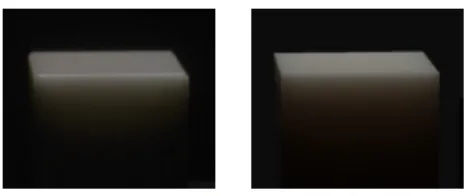
(a) (b)
Figure 8: Scattering of laser light in a marble block. The marble block is 40mm. wide and has a significant amount of subsurface scattering. The picture on the left is a photograph of the marble block, and the picture on the right is a synthetic rendering of a sim-ilarly sized cube using the BSSRDF model and the measured scat-tering properties of the marble. Note how the appearance of the two images is very similar.
Diffusion approximation for arbitrary geometry: An impor-tant component of the diffusion approximation is the use of the dipole source. If the geometry is locally flat we can get a very good approximation by using a similar dipole source configuration as that for flat materials (i.e., we always place the light source1/σ0t straight belowxi). Special care must be taken in the presence of highly curved surfaces; we handle this case by always evaluating the diffusion term with a minimum distance of1/σt0. In this way we eliminate singularities at sharp edges where the source can be placed arbitrarily close toxo. We found this approach to work very well in our experiments.
Texture: We approximate textured materials by making a few small changes to the usage of the BSSRDF. We only consider tex-ture variation at the surface — effects due to volumetric textex-ture variation would require a full participating media simulation. For the diffusion approximation we always use the material parameters atxi, which ensures a natural local blending of the texture proper-ties. For the single scattering term we useσs(xo)andσt(xo)along the refracted outgoing ray, andσt(xi)along the refracted incident ray. This variation is included in Equation 6.
5
Results
We have implemented the BSSRDF model in a Monte Carlo ray tracer, and in this section we will present a number of experimen-tal results obtained with this implementation. All simulations have been done on a dual 800MHz Pentium III PC running Linux and the images have been rendered with 4 samples per pixel and a width of 1024 pixels.
Our first simulation is shown in Figure 8, which compares a side photograph of a marble cube illuminated from above with a synthetic rendering. The synthetic image is rendered using the BSSRDF model and the measured parameters for marble (from the table in Figure 5). We only used a simple cube to approximate the rounded marble block, so there are natural visible differences along the edges. Nonetheless, the BSSRDF model faithfully renders the appearance including the scattered light exiting from the side of the marble cube.
Figure 9 shows several different simulations of subsurface scat-tering in a marble bust (1.3 million triangles) illuminated from be-hind. The BSSRDF simulation mostly matches the appearance of the full Monte Carlo simulation, yet is significantly faster (5 min-utes vs. 1250 minmin-utes). The hair at the back of the head is slightly darker in the BSSRDF simulation; we believe this is due to the forced1/σt0distance in the diffusion approximation. A similar ren-dering was done using photon mapping in [5] in roughly 12 min-utes (scaled to the speed of our computer). However, the photon mapping method requires a full 3D-description of the material, it requires memory to store the photons, and it becomes costly for
(a) (b) (c)
(d) (e) (f)
Figure 9: A simulation of subsurface scattering in a marble bust. The marble bust is illuminated from behind and rendered using: (a) the BRDF approximation (in 2 minutes), (b) the BSSRDF approximation (in 5 minutes), and (c) a full Monte Carlo simulation (in 1250 minutes). Notice how the BSSRDF model matches the appearance of the Monte Carlo simulation, yet is significantly faster. The images in (d–f) show the different components of the BSSRDF: (d) single scattering term, (e) diffusion term, and (f) Fresnel term.
highly scattering materials (such as milk and skin).
A particularly interesting aspect of the BSSRDF simulation is that it is able to capture the smooth appearance of the marble sur-face. In comparison the BRDF simulation gives a very hard ap-pearance where even tiny bumps on the surface are visible (this is a classic problem in realistic image synthesis where objects often look hard and unreal).
For the marble we used synthetic scattering and absorption co-efficients, since we wanted to test the difficult case when the av-erage scattering albedo is 0.5 (here the contribution from diffusion and single scattering is approximately the same). Figure 9 demon-strates how the sum of both single scattering and the diffusion term is necessary to match the Monte Carlo simulation.
Figure 10 contains three renderings of milk. The first render-ing uses a diffuse reflection model; the others use the BSSRDF model and our measurements for skim milk and whole milk. Notice how the diffuse milk looks unreal and too opaque compared to the BSSRDF images, even though multiple scattering dominates and the radiant exitance due to subsurface scattering is very diffuse. It is interesting that the BSSRDF simulations are capable of capturing the subtle details in the appearance of milk, making the milk look more bluish at the front and more reddish at the back. This is due to Rayleigh scattering that causes shorter wavelengths of light to be scattered more than longer wavelengths.
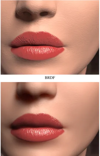
Skin is a material that is particularly difficult to render using methods that simulate subsurface scattering by sampling ray paths through the material. This is due to the fact that skin is highly scattering (typical albedo is 0.95) and also very anisotropic (typi-cal average cosine of the scattering angle is 0.85). Both of these properties mean that the average number of scattering events of a photon is very high (often more than 100). In addition skin is very translucent, and it cannot be rendered correctly using a BRDF (see Figure 11). A complete skin model requires multiple layers, but a
reasonable approximation can be obtained using just one layer. In Figure 11 we have rendered a simple face model using the BSSRDF and our measured values for skin (skin1). Here we also used the Henyey-Greenstein phase function [11] withg= 0.85as the esti-mated mean cosine of the scattering angle. The skin measurements are from an arm (which is likely more translucent than skin on the face), but the overall appearance is still realistic considering the lack of spatial variation (texture). The BSSRDF gives the skin a soft ap-pearance, and it renders the color bleeding in the shadow region below the nose. Here, the absorption by blood is particularly no-ticeable as the light that scatters deep in the skin is redder. For this simulation the diffusion term is much larger than the single scat-tering term. This means that skin reflects light fairly diffusely, but also that internal color bleeding is an important factor. The BRDF image was rendered in 7 minutes, the BSSRDF image was rendered in 17 minutes.
6
Conclusion and Future Work
In this paper we have presented a new practical BSSRDF model for computer graphics. The model combines a dipole diffusion ap-proximation with an accurate single scattering computation. We have shown how the model can be used to measure the scattering properties of translucent materials, and how the measured values can be used to reproduce the results of the measurements as well as synthetic renderings. We evaluate the BSSRDF by sampling the incoming light over the surface, and we demonstrate how this tech-nique is capable of capturing the soft and smooth appearance of translucent materials.
In the future we plan to extend the model to multiple layers as well as include support for efficient global illumination.
(a) (b) (c)
Figure 10: A glass of milk: (a) diffuse (BRDF), (b) skim (BSSRDF) and (c) whole (BSSRDF). (b) and (c) are using our measured values. The rendering times are 2 minutes for (a), and 4 minutes for (b) and (c); this includes caustics and global illumination on the marble table and a depth-of-field simulation.
BRDF
BSSRDF
Figure 11: A face rendered using the BRDF model (top) and the BSSRDF model (bottom). We used our measured values for skin (skin1) and the same lighting conditions in both images (the BRDF image also includes global illumination). The face geometry has been modeled by hand; the lip-bumpmap is handpainted, and the bumpmap on the skin is based on a gray-scale macro photograph of a piece of skin. Even with global illumination the BRDF gives a hard appearance. Compare this to the faithful soft appearance of the skin in the BSSRDF simulation. In addition the BSSRDF captures the internal color bleeding in the shadow region under the nose.
7
Acknowledgements
Special thanks to Steven Stahlberg for modeling the face. Thanks to the SIGGRAPH reviewers and to Maryann Simmons and Heidi Marschner for helpful comments on the manuscript. This research was funded in part by the National Science Foundation Information Technology Research grant (IIS-0085864). The first author was also supported by DARPA (DABT63-95-C-0085), and the second author was also supported by Honda North America, Inc.
References
[1] S. Chandrasekhar. Radiative Transfer. Oxford Univ. Press, 1960.
[2] R. L. Cook, T. Porter, and L. Carpenter. Distributed ray tracing. In ACM
Com-puter Graphics (SIGGRAPH’84), volume 18, pages 137–145, July 1984.
[3] P. Debevec, T. Hawkins, C. Tchou, H. Duiker, W. Sarokin, and M. Sagar. Acquir-ing the reflectance field of a human face. In Computer Graphics ProceedAcquir-ings,
Annual Conference Series, 2000, pages 145–156, July 2000.
[4] P. E. Debevec and J. Malik. Recovering high dynamic range radiance maps from photographs. In Computer Graphics Proceedings, Annual Conference Series,
1997, pages 369–378, August 1997.
[5] J. Dorsey, A. Edelman, H. W. Jensen, J. Legakis, and H. K. Pedersen. Modeling and rendering of weathered stone. In Computer Graphics Proceedings, Annual
Conference Series, 1999, pages 225–234, August 1999.
[6] G. Eason, A. Veitch, R. Nisbet, and F. Turnbull. The theory of the backscattering of light by blood. J. Physics, 11:1463–1479, 1978.
[7] W. G. Egan and T. W. Hilgeman. Optical Properties of Inhomogeneous
Materi-als. Academic Press, New York, 1979.
[8] T. J. Farell, M. S. Patterson, and B. Wilson. A diffusion theory model of spatially resolved, steady-state diffuse reflectance for the noninvasive determination of tissue optical properties in vivo. Med. Phys., 19:879–888, 1992.
[9] R. A. Groenhuis, H. A. Ferwerda, and J. J. Ten Bosch. Scattering and absorption of turbid materials determined from reflection measurements. 1: Theory. Applied
Optics, 22:2456–2462, 1983.
[10] P. Hanrahan and W. Krueger. Reflection from layered surfaces due to subsur-face scattering. In ACM Computer Graphics (SIGGRAPH’93), pages 165–174, August 1993.
[11] L. G. Henyey and J. L. Greenstein. Diffuse radiation in the galaxy. Astrophysics
Journal, 93:70–83, 1941.
[12] A. Ishimaru. Wave Propagation and Scattering in Random Media, volume 1. Academic Press, New York, 1978.
[13] G. Kortum. Reflectance Spectroscopy. Springer-Verlag, 1969.
[14] F. E. Nicodemus, J. C. Richmond, J. J. Hsia, I. W. Ginsberg, and T. Limperis. Geometric considerations and nomenclature for reflectance. Monograph 161, National Bureau of Standards (US), October 1977.
[15] M. Pharr and P. Hanrahan. Monte Carlo evaluation of non-linear scattering equa-tions for subsurface reflection. In Computer Graphics Proceedings, Annual
Con-ference Series, 2000, pages 75–84, July 2000.
[16] L. Reynolds, C. Johnson, and A. Ishimaru. Applied Optics, 15:2059, 1976. [17] J. Stam. Multiple scattering as a diffusion process. In Eurographics Rendering