5REXVWHVWLPDWLRQIRURUGLQDOUHJUHVVLRQ
&&URX[*+DHVEURHFNDQG&5XZHW
DEPARTMENT OF DECISION SCIENCES AND INFORMATION MANAGEMENT (KBI)
Robust estimation for ordinal regression
C. Crouxa,∗, G. Haesbroeckb, C. Ruwetb
a
KULeuven, Faculty of Business and Economics, Leuven, Belgium b
University of Liege, Department of Mathematics, Liege, Belgium
Abstract
Ordinal regression is used for modelling an ordinal response variable as a function of some explanatory variables. The classical technique for estimat-ing the unknown parameters of this model is Maximum Likelihood (ML). The lack of robustness of this estimator is formally shown by deriving its breakdown point and its influence function. To robustify the procedure, a weighting step is added to the Maximum Likelihood estimator, yielding an estimator with bounded influence function. We also show that the loss in efficiency due to the weighting step remains limited. A diagnostic plot based on the Weighted Maximum Likelihood estimator allows to detect outliers of different types in a single plot.
Keywords: Breakdown point, Diagnostic plot, Influence function, Ordinal regression, Weighted Maximum Likelihood, Robust distances.
1. Introduction
Logistic regression is frequently used for classifying observations into two groups. When dealing with more than two groups, this model needs to be
∗Corresponding author
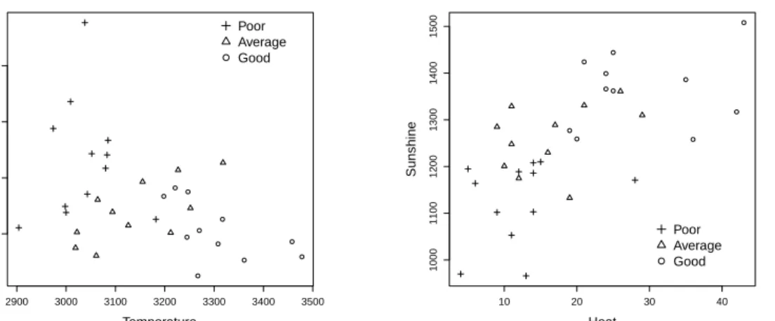
generalized. When the labels of these groups are naturally ordered, an ordi-nal regression model can be fitted to the data. The group label is then the ordinal response variable. Ordinal variables occur frequently in practice, e.g. in surveys where respondents have to specify whether they strongly disagree, disagree, are indifferent, agree or strongly agree with a given statement. As illustration in this paper, we use the wine data set of Bastien et al. (2005). These data characterize the quality of 34 years of Bordeaux wine, the qual-ity being assessed on the ordinal scale Poor-Average-Good. The qualqual-ity is assumed to be related to four explanatory variables: temperature (measured by the sum of average day temperatures in degrees celsius), sunshine (dura-tion of sunshine in hours), heat (number of very warm days) and rain (rain height in mm). In Figure 1, two scatter plots representing the data are given. One can see that the explanatory variables contain relevant information to characterize the quality of the wine. For example, rainy years correspond generally to poor wines as well as years with few sunshine and warm days.
Following Anderson and Philips (1981), we introduce the ordinal regres-sion model of interest via a latent, unobservable continuous variable Y∗.
This latent variable depends on a vector of explanatory variables X = (X1, . . . , Xp)t as
Y∗ =βtX+ε, (1)
where β is a p-vector of unknown regression parameters and ε is a random variable with cumulative distribution functionF. The observed ordinal vari-able Y takes as values the labels 1, . . . , J. We have
2900 3000 3100 3200 3300 3400 3500 300 400 500 600 Temperature Rain Poor Average Good 10 20 30 40 1000 1100 1200 1300 1400 1500 Heat Sunshine Poor Average Good
Figure 1: Scatter plots of Rain versus Temperature (left panel) and Sunshine versus Heat (right panel) for the Wine data categorized as Poor, Average or Good. The value of the dependent variable “quality of Wine” is represented by the corresponding symbol.
where the αj are unobserved thresholds with−∞=α0 < α1 < . . . < αJ−1 <
αJ =∞.Combining (1) and (2) yields
IP[Y =j|X =x] =F αj−βtx
−F αj−1−βtx
for j = 1, . . . , J. (3) We assume that F is strictly increasing and symmetric around zero, so
F(0) = 0.5. Standard choices for the distribution function F are the logistic link function, F(t) = 1/(1 +e−t), corresponding to the logistic distribution,
or the probit link function, F(t) = Φ(t), with Φ the cdf of the standard normal distribution.
Fitting an ordinal regression model requires the estimation ofJ−1+p pa-rameters, i.e. theJ−1 thresholdsα= (α1, . . . , αJ−1)t and thepcomponents
of β. Maximizing the log-likelihood function is the most common procedure to obtain these estimations (e.g. Anderson and Philips, 1981; Franses and Paap, 2001; Powers and Xie, 2008).
In general, when estimating parameters by means of Maximum Like-lihood, it is expected that outliers will have a devastating impact on the results. The lack of robustness of the Maximum Likelihood method in the logistic regression model has been already extensively studied in the litera-ture, e.g. breakdown points have been computed (e.g. Croux et al., 2002; M¨uller and Neykov, 2003) and influence functions have been derived (Croux and Haesbroeck, 2003). Also, robust estimation techniques have been intro-duced (e.g. Carroll and Pederson, 1993; Wang and Carroll, 1995; Bianco and Yohai, 1996; Gervini, 2005; Bondell, 2008; Hobza et al., 2008; Hosseinian and Morgenthaler, 2011). However, to our best knowledge, similar results are not yet available for the ordinal regression model.
In this paper, we investigate the lack of robustness of the ML procedure in the ordinal regression setting by computing breakdown points and influ-ence functions. A robust alternative consisting of a weighting step added to the ML methodology is then presented. Section 2 defines the Maximum Likelihood estimator and states the conditions under which this estimator exists. In Section 3, the breakdown point of the ML estimator is derived and shown to go to zero as the sample size tends to infinity. A robust alternative is introduced in Section 4. In Section 5, the influence functions of the clas-sical and robust estimators are computed and they are then used in Section 6 to construct a diagnostic plot detecting influential points. The statistical precision of the robust estimators is discussed in Section 7. Finally, Section 8 makes some conclusions.
2. Maximum likelihood estimation
2.1. Definition
Let Zn = {(xi, yi) : i = 1, . . . , n} be a sample of size n where the vector xi ∈ Rp contains the observed values of the p explanatory variables and yi,
with 1 ≤ yi ≤ J, indicates the membership to one of the J groups. The
Maximum Likelihood estimator is obtained by maximizing the log-likelihood function, i.e.
( ˆα,βˆ) = argmax
(α,β)∈RJ−1+p
l(α, β), (4) under the constraint α1 < . . . < αJ−1, with
l(α, β) = n X i=1 J X j=1 δijlog F αj −βtxi −F αj−1−βtxi , (5) and where the indicator function δij takes the value 1 when yi = j and 0
otherwise.
To explicitly take into account the ordering constraint in the maximiza-tion, Franses and Paap (2001) recommend to re-parameterize the log-likeli-hood function by replacing the vector of thresholds α by γ = (γ1, . . . , γJ−1)t
defined as α1 = γ1 αj = γ1+ j X k=2 γk2, for j = 2, . . . , J −1. (6) The parameterγ is uniquely identified by asking thatγj ≥0, for j >1. The
log-likelihood function (5) can be rewritten as l(γ, β) = n X i=1 J X j=1 δijlog F(γ1+ j X k=2 γ2k−βtxi)−F(γ1+ j−1 X k=2 γk2−βtxi) ! = n X i=1 ϕ(xi, yi,(γ, β)). (7)
The Maximum Likelihood estimators of γ and β are then given by (ˆγ,βˆ) = argmax
(γ,β)∈RJ−1+p
l(γ, β). (8) The advantage of the optimization problem in (8) is that no constraints need to be put on the parameters: the resulting estimates for the thresholds αwill be automatically ordered. Furthermore, equality of two thresholds implies a zero values for some γj, withj > 1, yielding minus infinity for the objective
functions in (7), and they can be excluded from the solutions set. 2.2. Existence
When working with a binary regression model, it is well known that an overlap between the two groups of observations is necessary and sufficient for existence and uniqueness of the Maximum Likelihood estimates (Albert and Anderson, 1984). For ordinal regression, the existence of the ML estimates has also been characterized by overlap conditions. Haberman (1980) states these conditions in algebraic terms. Proposition 1 below summarizes these conditions.
Proposition 1 (Haberman, 1980). Let the set Ij contain the indexes of the
observations for which yi = j, for j = 1, . . . , J. The Maximum Likelihood
(i) X
i
δij ≥1 for all j = 1, . . . , J
(ii) For all α and β, there exists an index j in {1, . . . , J}, and there exists an i in Ij such that xt
iβ < αj−1 or xtiβ > αj.
In words, these conditions state that the ML estimates exist if and only if (i) there is no empty group and (ii) there is overlap between at least two groups with consecutive labels. As only one overlap is necessary to ensure existence and uniqueness, the overlap condition is not more stringent than in the binary case.
3. Breakdown point of the Maximum Likelihood estimator
In the logistic regression setting, Croux et al. (2002) showed that the ML estimator never explodes when outliers are added to the data. On the other hand, the estimated slope goes to zero when adding 2pwell chosen outliers. This behavior also holds in ordinal regression, as Propositions 2 and 3 below prove.
Letzi = (xi, yi) denote the ith observation and Zn′+m ={z1, . . . , zn, zn+1,
. . . , zn+m}the initial sample withmoutliers, zn+1, . . . , zn+m,added. The ML
estimator of the thresholds and slope parameter is denoted by ˆθ(Zn) = ˆθn.
The notation k.krefers to the Euclidean norm.
Definition. The explosion breakdown point of ˆθn at the sample Zn is the
minimal fraction of outliers that needs to be added to the initial sample to get the estimator over all bounds, i.e.
ε+(ˆθn, Zn) = m+ n+m+ with m + = min m∈N0 zn+1sup,...,zn+mkθˆ(Zn′+m)k=∞ .
The above definition is the addition breakdown point of an estimator. Alternatively, once could consider the replacement breakdown point, where observations are replaced by outliers until the estimator goes over all bounds. The replacement breakdown point is less appealing in our setting, since one could make the overlap condition of proposition 1 fail, causing a breakdown of the estimator due to its non-existence. When adding outliers to the data, the overlap condition remains verified.
Assuming that overlap holds initially, Proposition 2 formally proves that the ML estimator in ordinal regression is uniformly bounded above when adding an arbitrary number of outliers in the data. The proof is given in the Appendix.
Proposition 2. Assume that kθˆ(Zn)k<∞, with θˆ(Zn) the Maximum
Like-lihood estimator computed on the sample Zn. Then ε+(ˆθn, Zn) = 1.
While Proposition 2 shows that the explosion breakdown point of the ML estimator is 100%, Proposition 3 derives an upper bound for the breakdown point of the slope estimator taking both implosion and explosion behaviors into account.
Definition. The breakdown point of ˆβn at the sample Zn is the minimal
fraction of outliers that needs to be added to the initial sample in order to make the estimator tend to zero or to infinity:
ε( ˆβn, Zn) = m∗
n+m∗
with m∗ = min(m+, m−) and
m+ = min m∈N0 zn+1sup,...,zn+m kβˆ(Zn′+m)k=∞
m− = min m∈N0 zn+1,...,zinfn+mk ˆ β(Zn′+m)k= 0 .
Proposition 3. At any sample Zn, the breakdown point of the slope of the
ML estimator for the ordinal regression model satisfies
ε( ˆβn, Zn)≤ pJ n+pJ,
where p is the number of explanatory variables and J the number of groups. Proposition 3 shows that the ML estimator is not robust since its asymp-totic breakdown point, i.e. limn→+∞ε( ˆβn, Zn), is zero. This lack of
robust-ness does not come from an explosion but rather from an implosion of the slope estimator toward zero. It is interesting to note that the implosion of the slope estimate does not imply implosion of the estimations of the thresh-olds. Indeed, as ˆβ goes to 0, ˆαj tends toF−1(p1+. . .+pj), wherepj is the
frequency of observations in the jth group. In general, this limit does not vanish to zero.
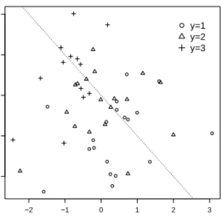
To illustrate the implosion breakdown of the slope estimator, let us con-sider the simulated data set pictured in Figure 2, with n = 50 observations classified into J = 3 ordered groups. The group membership depends on
p = 2 explanatory variables (simulated as independent standard normals) while the error term is distributed according to the logistic distribution. The true values of the parameters are set at β = (−1,1.5)t and α
1 =−α2 =−1.
This choice of thresholds leads to three groups of equivalent size. Based on this initial data set, the ML estimate of β is given by ˆβ = (−1.30,1.60)t,
yieldingkβˆk= 2.06. The ML estimator yields a misclassification rate (which is the proportion of observations for which ˆy6=y) equal to 28%.
−2 −1 0 1 2 3 −2 −1 0 1 2 X1 X2 y=1 y=2 y=3
Figure 2: Scatter plot of the simulated data set. The dotted line represents the shift of the additional observation ((s,−s),3).
Both the estimator and the misclassification rate may be completely per-turbed by the introduction of a single outlier in the data. Add one obser-vation with x = (s,−s) moving along the dotted line in Figure 2 and with
y = 3. This additional observation is most outlying when s is positive since it lies then in the region of observations associated with the smallest possi-ble y-score. When s is negative, the observation is outlying in the space of explanatory variable (if s is large) but it has the expected value as far as the
y-variable is concerned.
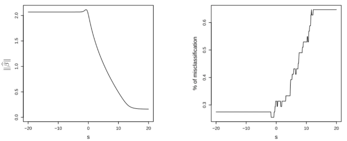
For each value of s, the parameters of the ordinal regression model are estimated by Maximum Likelihood and the corresponding misclassification rate is computed. The resulting norm of ˆβ and the rate of misclassification are represented in Figure 3 with respect tos.As expected, negative values ofs
yield an additional observation which does not bias too much the estimator. On the other hand, as soon as s gets positive, the impact of the added
−20 −10 0 10 20 0.0 0.5 1.0 1.5 2.0 s k bβk −20 −10 0 10 20 0.3 0.4 0.5 0.6 s % of misclassification
Figure 3: Simulated data set with ((s,−s),3) as additional observation. Left panel: Norm of the slope parameter. Right panel: Proportion of misclassified observations.
observation becomes apparent and gets even quite extreme as s increases. Not only the norm of the slope estimator goes to zero but the misclassification rate reaches a limit of about 66%, close to the classification performance of a random guess.
4. Weighted Maximum Likelihood Estimator
In this Section, we construct a robust alternative to the ML estimator. The most simple way to decrease the influence of outliers is to downweight them by adding weights into the log-likelihood function. As such, a weighted Maximum Likelihood estimator is obtained, as already suggested and studied in the simple logistic regression setting (e.g. Carroll and Pederson, 1993; Croux and Haesbroeck, 2003; Croux et al., 2008).
Many different types of weights could be designed. Here, the downweight-ing will be done usdownweight-ing robust distances computed in the space of the
ex-planatory variables. Let m and S denote robust estimates of the location and covariance matrix based on x1, . . . , xn. In this paper, the Minimum
Co-variance Determinant estimator (Rousseeuw and Van Driessen, 1999) with a breakdown point of 25% has been used. The weight wi attributed to theith
observation is then given by
wi =W(di) withdi = (xi−m)tS−1(xi−m), (9)
for a given weight functionW. The robust distances measure the outlyingness of each observation xi, for i = 1, . . . , n. They are only computed from the
continuous explanatory variables. In particular, dummy variables are not taken into account when computing the distances.
The Weighted Maximum Likelihood (WML) estimator is then the solu-tion of the following maximizasolu-tion problem
(ˆγ,βˆ) = argmax (γ,β)∈RJ−1+p n X i=1 wiϕ(xi, yi,(γ, β)), (10)
whereϕis the log-likelihood of an individual observations, as in equation (7). Obviously, if one takes a constant weight function, the usual ML es-timator is obtained again. A typical weight function is the step function
W0/1(d) = I(d ≤ χ2p(0.975)) where χ2(0.975) is the 97.5% quantile of the
chi-squared distribution withpdegrees of freedom. With such a weight func-tion, observations lying far away from the bulk of the data are discarded. As only extreme observations are discarded, one expects that in most cases the overlap condition of Proposition 1 will still hold. Nevertheless, to guarantee existence of overlap, a smoother weight function is prefered, as the Student weight function defined by Wν(d) = (p+ν)/(d+ν), where ν is the degree
of freedom. The larger ν, the less observations are downweigthed. We take
ν = 3. Far away observations do get small weights but are not discarded completely from the data set. Therefore, the weighted ML estimate using the W3 weight function exists as soon as the ML estimate exists.
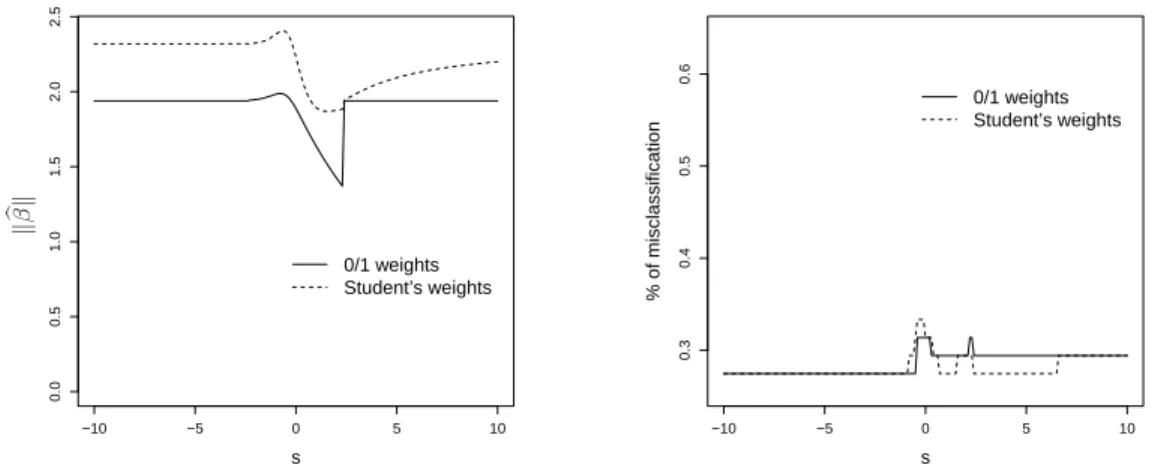
To illustrate numerically the robustness of the WML estimator, we repeat the experiment discussed in Section 3. Similar as Figure 3, Figure 4 shows how the norm of a robust estimate of the slope parameter depends on the position of a single added outlier with value x = (s,−s)t and y = 3. It
can be seen that the norm of the slope does not tend to zero anymore, and is only changing in the region where the added observation is not too different from the bulk of the data. We see that the curve corresponding to the Student weight function is smoother than the one based on the 0/1 weights, as expected. Figure 4 also shows that the misclassification rate is only slightly varying with the values of the outlier, and nowhere close to 66%, the misclassification rate corresponding to random guessing.
5. Influence function
5.1. Derivation
Breakdown points are global measures of robustness measuring robust-ness in presence of large amounts of contamination. On the other hand, influence functions are local measures of robustness, characterizing the im-pact of an infinitesimal proportion of contamination located at a point (x, y). The influence function of a statistical functional T at the model distribution
H0 is defined by
IF((x, y);T, H0) = lim
ε→0
T((1−ε)H0+ε∆(x,y))−T(H0)
−10 −5 0 5 10 0.0 0.5 1.0 1.5 2.0 2.5 s 0/1 weights Student’s weights k bβk −10 −5 0 5 10 0.3 0.4 0.5 0.6 s % of misclassification 0/1 weights Student’s weights
Figure 4: Simulated data set with ((s,−s),3) as additional observation. Left panel: Norm of the slope parameter. Right panel: Proportion of misclassified observations. Parameters are estimated with WML using 0/1 weights (solid line) or Student’s weights (dashed line).
where ∆(x,y) is the Dirac distribution having all its mass at (x, y) for given
x ∈IRp and y ∈ {1, . . . , J}. Contamination on y is restricted to its possible
values since any other choice for y would be easily detected.
We first derive the influence function of the statistical functionals related to the estimation of the parameters γ and β. They are the solutions of an unconstrained problem, see equation (8), and easier to deal with. Let θ
represent the joint vector (γ, β). The statistical functional relative to the ML estimator in ordinal regression is given by
θM L(H) = argmax θ∈RJ−1+p
EH[ϕ(X, Y;θ)],
for any distribution H of the variables (X, Y). The first order condition yields
EH[ψ(X, Y;θ)] = 0 with ψ(X, Y;θ) =
∂ϕ(X, Y;θ)
At the model distributionH0, equation (3) holds, and it follows thatθM L(H0) =
θ0, with θ0 the true parameter vector. We observe that θM L is simply a
M-type statistical functional for which the IF is readily available (Hampel et al., 1986, page 230) and given by:
IF((x, y);θM L, H0) =−EH0 " ∂2ϕ(X, Y;θ) ∂θ2 θ0 #−1 ψ(x, y;θ0). (12)
The first factor in (12) is a constant (J−1 +p)-square matrix, which we demote by M(ψ, H0), independent of x and y. Its explicit form is given in
the Appendix. The shape of the influence function is mainly determined by the second factor ψ with components (ψ1, . . . , ψJ−1, ψβ), and defined as
ψ1(x, y;θ) = J X j=1 I(y=j)f(αj−β tx)−f(α j−1−βtx) F(αj−βtx)−F(αj−1−βtx) , ψk(x, y;θ) = 2γk I(y =k) f(αk−β tx) F(αk−βtx)−F(αk−1−βtx) + J X j=k+1 I(y=j)f(αj−β tx)−f(α j−1−βtx) F(αj−βtx)−F(αj−1−βtx) # for k = 2, . . . , J −1 and ψβ(x, y;θ) =−x J X j=1 I(y=j)f(αj−β tx)−f(α j−1−βtx) F(αj−βtx)−F(αj−1−βtx) ,
with f =F′ the density function of the error term in (1).
It is easy to see that the influence function of ML is bounded iny, sincey
only enters the IF through the indicator functions I(y =j). The first J−1 components of ψ are also bounded in x, as f and F are bounded functions (at least for the logit and probit link functions). The slope component of ψ, however, is unbounded in the value of the covariate x, proving the lack of
robustness of the ML-estimator in presence of small amounts of contamina-tion.
Let us now turn to the derivation of the influence function of the WML statistical functional θW M L. It is defined as
θW M L(H) = argmax θ∈RJ−1+p
EH[W(DH(X))ψ(X, Y;θ)]
where (X, Y) ∼ H. With GH the marginal distribution of X, the distance
function DH is given by DH(x) = (x−µ(GH))tΣ(GH)−1(x−µ(GH)) where
(µ(GH),Σ(GH)) are the location and covariance functionals corresponding
to the MCD estimator.
Using the explicit expression of ψ given above, it is easy to check that conditional Fisher consistency holds, i.e. EH0[ψ(X, Y;θ0)|X =x] = 0 for
all x ∈ Rp. Lemma 1 of Croux and Haesbroeck (2003) leads then to the
following expression for the influence function, IF((x, y);θW M L, H0), of the
Weighted Maximum Likelihood estimator:
−EH0 " W(DH0(X)) ∂2ϕ(X, Y;θ) ∂θ2 θ0 #−1 W(DH0(x))ψ(x, y;θ0). (13)
Leaving aside the constant matrix, the impact of an infinitesimal con-tamination at (x, y) on WML is measured by means of the same function ψ
as before, now multiplied by the weight function. The influence function of WML remains therefore bounded in y but also becomes bounded with re-spect to outlying values of the explanatory variables as soon asx W(DH0(x))
is bounded. Both for the Student weight function and for the 0/1 weight function we get bounded influence functions.
From expressions (12) and (13), the influence functions of the functionals corresponding to the thresholds α1, . . . , αJ−1, are readily obtained. Denote
A1, . . . , AJ−1the statistical functionals corresponding to the estimators of the
components of the parameter α, andC1, . . . , CJ−1 the firstJ−1 components
of the statistical functional θM L or θW M L. Using definition (6), one gets
IF ((x, y) ;A1, H0) = IF ((x, y) ;C1, H0) IF ((x, y) ;Aj, H0) = IF ((x, y) ;C1, H0) + 2 j X k=2 γkIF ((x, y) ;Ck, H0) for j = 2, . . . , J −1. 5.2. Numerical Illustrations
Let us look at some graphical representations of the influence functions. We take for F the probit link but similar results hold for the logit link. We consider the model Y∗ =βtX+ε, where the covariates X follow a standard
normal distribution. The ordinal variable Y is then given by (2), where the thresholds are such that every group has equal probability of occurrence.
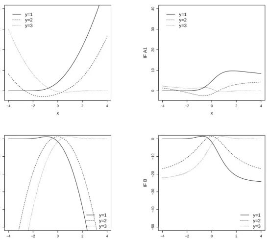
We focus here on the univariate case, p = 1, with J = 3 groups and we set β = 1.5. Figure 5 shows the influence functions of A1 (upper panels) and
of the functional B estimating the slope parameter β (lower panels) for the ML estimator (left panels) and for the WML estimator based on Student’s weights with ν = 3 (right panels), as a function of x. Several curves are drawn, one for each possible value of y. While the influence functions of the ML estimator are unbounded, adding weights yields bounded influence functions for the WML estimator. Bounded IF are also obtained for the WML estimator with the 0/1 weighting scheme (not reported) but jumps appear due to the discontinuity of the step weight function.
−4 −2 0 2 4 0 10 20 30 40 x IF A1 y=1 y=2 y=3 −4 −2 0 2 4 0 10 20 30 40 x IF A1 y=1 y=2 y=3 −4 −2 0 2 4 −50 −40 −30 −20 −10 0 x IF B y=1 y=2 y=3 −4 −2 0 2 4 −50 −40 −30 −20 −10 0 x IF B y=1 y=2 y=3
Figure 5: Influence functions for the first threshold A1 (upper row) and for the slope B (lower row) as functions of xwith y ∈ {1,2,3}, forp= 1 and with J = 3 groups. Left panels: ML estimator. Right panels: WML estimator based on Student weight function withν = 3.
It is worth to interpret in more detail these influence functions. First, as
β is positive, large negative values of the explanatory variable yield a fitted value of the ordinal variable, ˆy, equal to its smallest score (ˆy = 1) while large positive ones would correspond to the highest score (ˆy = 3). Looking now at the influence function of the first threshold (upper plots of Figure 5), one can observe that negative (resp. positive) x values have a zero influence when associated with y = 1 (resp. y = 3), showing that these points are not influential even on the ML estimator. The influence is smaller (in absolute value) for those x lying in the area corresponding to ˆy = y than elsewhere. The same remarks hold for the IF of the slope parameter (see lower panel of Figure 5). These influence functions also shows the expected symmetry.
This leads to the definition of several types of outliers in the ordinal regression setting. For outlying values of x, i.e. for leverage points, some couples (x, y) are influential, while others are not. If ˆy=y, the corresponding outlier has less influence on the estimation of the parameters. It can be labelled as a good leverage point, as in linear regression (Rousseeuw and Leroy, 1987). On the other hand, when ˆy 6= y, this outlier might be highly influential and can be considered as abad leverage point. It may happen that ˆ
y 6=y even if x is not outlying in the space of the explanatory variables. In that case, we talk about vertical outliers.
6. Diagnostic plot
It has been shown that atypical observations may have an important effect on the Maximum Likelihood estimator. In order to detect the potentially influential observations beforehand, diagnostic measures could be computed.
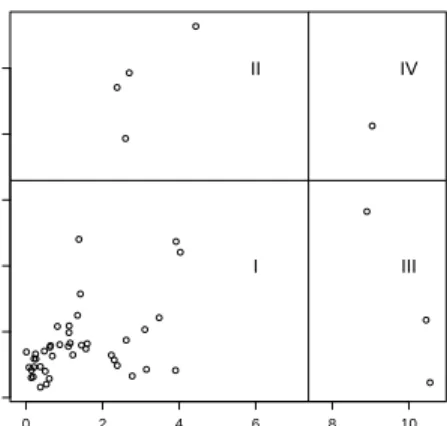
0 2 4 6 8 10 0 2 4 6 8 10 RD EIFB II IV III I
Figure 6: Illustration of the diagnostic plot detecting influential points (vertical axis) and leverage points (horizontal axis). The influence measure is plotted versus the robust distance (RD).
Here follow the approach of Pison and Van Aelst (2004), based on influence functions.
The influence of each observation on the classical estimator is measured and plotted with respect to the robust distances (RD) computed on the continuous explanatory variables in the data set. Figure 6 displays such a diagnostic plot. The vertical and horizontal lines correspond to cutoff values: a distance or influence measure larger than the cutoff value indicates an atypical observation. As shown on Figure 6, we get four parts: Part I contains the regular observations, Part II corresponds to the vertical outliers, part III to the good leverage points and Part IV to the bad leverage points. To compute the influence measures, we evaluate the influence function of the ML estimator at each observed couple (xi, yi). As expression (12) shows,
explanatory variables, G,and the true values of the parameters,θ0. To avoid
the masking effect, Pison and Van Aelst (2004) suggest to estimate G and
θ0 in a robust way. The parameter θ0 is estimated by WML. The
distribu-tion G is estimated by the empirical distribution based on the observations which are not detected as outliers in the space of explanatory variables, i.e. for which di ≤ χ2p(0.975). Recall that di are the robust distances defined
in (9). Since G and θ0 are replaced by estimates, we speak about empirical
influence functions (EIF). The overall influence measures for the threshold and regression slope estimators are then
EIFAi = k EIF((xi, yi), A)k √ J−1 and EIFBi = kEIF((xi, yi), B)k √p
where the factors 1/√J−1 and 1/√p scale the norms. As cutoff for the influence measure, the empirical 95% quantile of a set of simulated overall empirical influence functions is chosen, as in Pison and Van Aelst (2004).
Two examples will illustrate the usefulness of this diagnostic plot in prac-tice. The first one is based again on the simulated data set of Section 3. In this simple and simulated setting, the different types of outliers may be eas-ily detected by visual inspection of the data. We will show that the same detection may be obtained via the corresponding diagnostic plot.
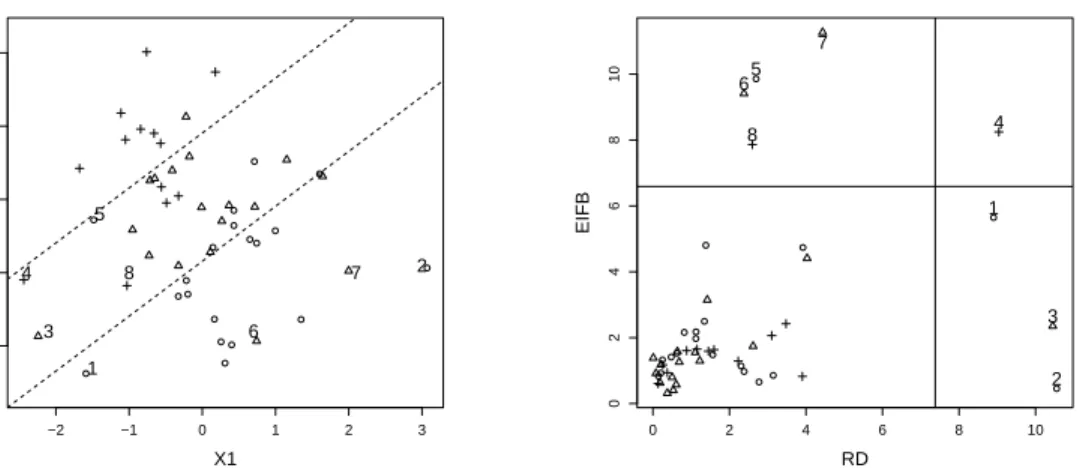
The left panel of Figure 7 displays the data together with the robust fit obtained with the Weighted Maximum Likelihood estimator. The dashed lines separate the plane in three parts, according to the fitted value of the respons variable. The diagnostic plot for the slope parameter is shown on the right panel (similar results hold for the thresholds). Some particular observa-tions (numbered from 1 to 8) are pinpointed on these two plots. Observaobserva-tions 1, 2, 3 and 4 are leverage points. Out of these four observations, only one
−2 −1 0 1 2 3 −2 −1 0 1 2 X1 X2 1 2 3 4 5 6 7 8 0 2 4 6 8 10 0 2 4 6 8 10 RD EIFB 1 2 3 4 5 6 7 8
Figure 7: Original simulated data set together with the fitted separating lines based on the WML estimator with 0/1 weights (left panel) and corresponding diagnostic plot (right panel).
(observation 4) is a bad leverage point. Observations labelled as 5, 6, 7 and 8 are not outlying in the space of explanatory variables but are misclassified. They are vertical outliers and lie indeed in Part II of the diagnostic plot.
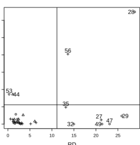
For the second illustration, let us come back to the wine data set presented in the Introduction. There are n = 34 observations and p = 4 explanatory variables; visual analysis of the data is no longer possible. Figure 8 gives the diagnostic plot based on the slope parameter. Several observations (num-bered by their index which gives the corresponding year of the production of the wine) lie in the outlying parts of the plot. Eight observations are out-lying in the space of explanatory variables. Two of them are bad leverage points (years 1928 and 1956) while the others (years 1927, 1929, 1932, 1935, 1947 and 1949) are not influential. Except for 1935, these years are known to be either disastrous or exceptional as far as their climatic conditions are
0 5 10 15 20 25 0 1 2 3 4 5 6 RD EIFB 27 28 29 32 35 44 47 49 53 56
Figure 8: Diagnostic plot for the Wine data set.
concerned. Years 1944 and 1953 are flagged as vertical outliers. They corre-spond indeed to wines for which the observed quality is not validated by the estimated model.
7. Simulation study
While adding weights in the log-likelihood function makes the ML es-timator robust, it also leads to a loss in statistical efficiency. By means of a modest simulation study, we show that this loss remains limited. For
m = 5000 samples of size n = 50 or n = 200, observations were generated according to the ordinal regression model, with F the probit link function, and the covariates following a N(0, Ip) distribution, for p= 2,3 and 5. The
thresholds α = (α1, . . . , αJ−1)t are selected such that every value of the
or-dinal variable Y has the same probability to occur. We present results for
J = 3 groups. The slope parameter is taken as β = (1,1, . . . ,1)t. For every
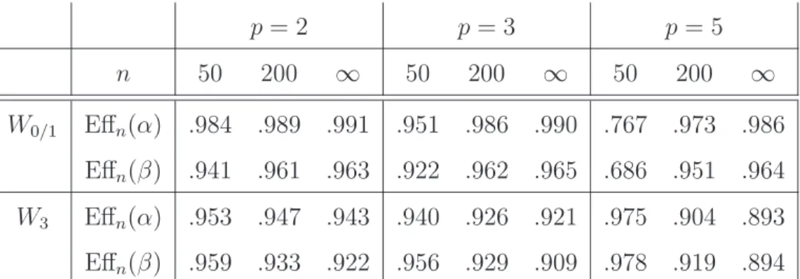
p= 2 p= 3 p= 5 n 50 200 ∞ 50 200 ∞ 50 200 ∞ W0/1 Effn(α) .984 .989 .991 .951 .986 .990 .767 .973 .986 Effn(β) .941 .961 .963 .922 .962 .965 .686 .951 .964 W3 Effn(α) .953 .947 .943 .940 .926 .921 .975 .904 .893 Effn(β) .959 .933 .922 .956 .929 .909 .978 .919 .894
Table 1: Relative efficiencies of WML w.r.t. ML for the threshold and slope estimators, using 0/1 weights (W0/1) and the Student weight function (W3).
both the 0/1 and the student weight functions.
For every component of α and β, we compute the Mean Squared Errors (MSE) of the estimators, and summarize the relative finite-sample efficiencies of the Weighted ML versus the ML estimator as
Effn(α) = 1 J −1 J−1 X k=1 MSE( ˆαk,M L) MSE( ˆαk,W M L) and Effn(β) = 1 p p X k=1 MSE( ˆβk,M L) MSE( ˆβk,W M L) .
The results are reported in Table 1. In the column n = ∞, we report asymptotic efficiencies computed using the rule
ASV(T, H0) = EH0
IF2((X, Y);T, H0)
,
with T the functional corresponding to the estimation of one component of
α orβ (Hampel et al., 1986, page 85). Using numerical integration and the expression for the influence functions derived in Section 5, we obtain the asymptotic variances and efficiencies.
Table 1 shows that the loss in efficiency remains very limited. When using the 0/1 weights, the efficiencies are above 90%, with the exception of
the setting where the sample size is low w.r.t. the dimension, i.e. p = 5 and n = 50. We also observe that the finite-sample efficiencies converge to their asymptotic counterparts. Using the smooth weight function W3
yields slightly lower efficiencies, but they are more stable with respect to the sample size. We observe again convergence to the asymptotic efficiencies. We conclude from this simulation study that the loss in statistical efficiency when using the WML is very limited, while, as shown in the previous section, it has much better robustness properties.
8. Conclusion
To the best of our knowledge, this is the first paper where robustness for ordinal regression is studied. First we study the robustness of the classical Maximum Likelihood Estimator, and show that the slope estimator is explo-sion robust but implodes toward zero when well-chosen outliers are added to the data. We also showed that the ML estimator has an unbounded in-fluence function, but the IF remains bounded with respect to contamination in the ordinal response variable. To obtain a bounded influence estimator, it therefore suffices to add weights based on the outlyingness of the values of the explanatory variables. The resulting Weighted Maximum Likelihood estimator has a bounded IF if the weight function is appropriately chosen. The price for the gain in robustness when using the WML is a loss in statisti-cal efficiency. However, as shown in Section 7, this loss in efficiency remains limited.
The influence functions are not only useful in their own right but may also be used to compute asymptotic variances of the classical and robust
estimators, as was done in Section 7. Furthermore, the influence functions can be used in a diagnostic context, as shown in Section 6: combining robust distances with influence measures, one can detect different types of outliers (vertical outliers, good and bad leverage points) in a single diagnostic plot.
Appendix
Expression for the constant matrix M(ψ, H0) in (12)
The matrix M(ψ, H0) can be decomposed as
m11 m12 m13 m14 . . . m1(J−1) M1B m12 m22 2γ2m13 2γ2m14 . . . 2γ2m1(J−1) M2B m13 2γ2m13 m33 2γ3m14 . . . 2γ3m1(J−1) M3B ... ... . .. ... ... m1(J−1) 2γ2m1(J−1) 2γ3m1(J−1) . . . m(J−1)(J−1) M(J−1)B Mt 1B M2tB . . . M(tJ−1)B MBB .
Let X ∼GH, then m11 =−EGH " J X j=1 (f(αj −βtX)−f(αj−1−βtX))2 F(αj −βtX)−F(αj−1−βtX) # , m1k =−2γk EGH f(αk−βtX)(f(αk−βtX)−f(αk−1−βtX)) F(αk−βtX)−F(αk−1−βtX) + J X j=k+1 EGH (f(αj −βtX)−f(αj−1−βtX))2 F(αj−βtX)−F(αj−1−βtX) ) , M1B =EGH " X J X j=1 (f(αj −βtX)−f(αj−1−βtX))2 F(αj−βtX)−F(αj−1−βtX) # , MkB = 2γk EGH X f(αk−βtX)(f(αk−βtX)−f(αk−1−βtX)) F(αk−βtX)−F(αk−1−βtX) + J X j=k+1 EGH (f(αj −βtX)−f(αj−1−βtX))2 F(αj−βtX)−F(αj−1−βtX) ) ,
for k = 2, . . . , J −1. Furthermore, the diagonal elements are given by
mkk =−4γk2 EGH f(αk−βtX)2 F(αk−βtX)−F(αk−1−βtX) + J X j=k+1 EGH (f(αj −βtX)−f(αj−1−βtX))2 F(αj−βtX)−F(αj−1−βtX) ) for k = 2, . . . , J −1, and MBB =−EGH " XtX J X j=1 (f(αj −βtX)−f(αj−1−βtX))2 F(αj−βtX)−F(αj−1−βtX) # .
To obtain the constant matrix in (13), we add the weight W(DH(X)) in all
the expectations.
Proofs of the Propositions
Proof of Proposition 2 In order to prove this, let us show that for every
such that
sup
zn+1,...,zn+m
kθˆ(Zn′+m)k< M(Zn, m).
For every θ = (α1, . . . , αJ−1, βt)t, define
δ(θ, Zn) = inf{ρ >0| ∃j ∈ {1, . . . , J −1}and ∃i∈Ij+1:xtiβ ≤ −ρ+αj
ori∈Ij :xitβ ≥ρ+αj}.
The existence conditions stated in Proposition 1 imply that 0 < δ(θ, Zn)<
+∞. This can also be written as max j=1,...,J−1{rj0(θ),−rj1(θ)}, whererj0 = min Ij max(x t iβ−αj,0) andrj1 = max Ij+1 min(x t iβ−αj,0). Thus, the
mapping θ→δ(θ, Zn) is continuous. Then, withSp+J−2 denoting the sphere
in Rp+J−1 centered at the origin, one getsδ∗(Z
n) = inf θ∈Sp+J−2
δ(θ, Zn)>0.
Denote the log-likelihood function on the contaminated sample Z′
n+m as l. Let l0 be this log-likelihood computed for the vector θ∗ = (α∗, β∗) with
α∗
j = F−1(j/J), j = 1, . . . , J −1 and β∗ = 0. It is easy to check that l0 =−(n+m) logJ. Take ˜z = exp(l0) and define
M(Zn, m) =
F−1(1−z˜)
δ∗(Z
n) ,
which only depends on the original sample Zn and on the number m of
outliers added to Zn. Let us suppose that ˆθn+m satisfies
kθˆn+mk> M(Zn, m). (14)
For all ˆθn+m ∈ RJ−1+p, there exist at least one j0 ∈ {1, . . . , J −1} and
one 1≤i0 ≤n such that
i0 ∈Ij0 and xt i0βˆn+m−αcj0n+m kθˆn+mk ≥δ θˆn+m kθˆn+mk , Zn ! ≥δ∗(Zn)>0 (15)
or i0 ∈Ij0+1 and xt i0βˆn+m−αcj0n+m kθˆn+mk ≤ −δ θˆn+m kθˆn+mk , Zn ! ≤ −δ∗(Zn)<0. (16) Case 1: Wheni0 verifies (15), the log-likelihood is such that
l(ˆθn+m;Zn′+m) = nX+m i=1 L(ˆθn+m;zi)≤L(ˆθn+m;zi0) since L(θ;zi) = J X j=1 δijlog F(αj−βtxi)−F(αj−1−βtxi) is always nega-tive. Thus, l(ˆθn+m;Zn′+m)≤log h F αcj0n+m−x t i0βˆn+m −F α[j0−1 n+m−x t i0βˆn+m i ≤loghF αcj0n+m−x t i0βˆn+m i ≤loghF −kθˆn+mkδ∗(Zn) i = logh1−F kθˆn+mkδ∗(Zn) i <log [1−F (M(Zn, m)δ∗(Zn))] = log(˜z) =l0
using the inequalities in (15), the symmetry and strict increasing behavior of
F, the hypothesis thatkθˆn+mk> M(Zn, m) and the definitions ofM(Zn, m)
and ˜z.
Case 2: When i0 verifies (16), one also gets l(ˆθn+m;Zn′+m) < l0. Here
the inequality log(y−x)<log(1−x) for 0 < x < y <1 is used.
The inequality l(ˆθn+m;Zn′+m)< l0 implies that ˆθn+m cannot be the
ML-estimate. Therefore, equation (14) does not hold and the theorem is proven.
Proof of Proposition 3As in the previous proof, letlbe the log-likelihood
function on the contaminated sample Z′
Let δ > 0 be fixed. It is always possible to find ξ > 0 s.t. log(F(−ξ)) = l0.
Let us define M = max
1≤i≤nkxik, N = ξ/δ and A =
√p(2N +M). Take {e1, . . . , ep} the canonical basis of Rp and add to the initial sample Zn the m =pJ outliers
zij = (vit, j) withvi =A ei, i= 1, . . . , p and j = 1, . . . , J.
Take kβk > δ, α arbitrarily and θ = (α, β). The aim is to show that
l(θ;Z′
n+m) < l0 as soon as kβk > δ which will imply that kβˆn+mk ≤ δ.
Since this reasoning holds for all δ >0, ˆβ can be made as small as possible by adding m =pJ outliers.
For j fixed in {1, . . . , J − 1}, define the hyperplane Hδj = {x ∈ Rp : αj −xtβ = 0}. The distance between a vector x∈Rp and Hδj is
dist(x, Hδ) = xtkββk − kαβjk .
First, suppose that∃i0 ∈ {1, . . . , p}s.t. dist(vi0, H
j
δ) is bigger than N. If αj−vti0β > 0, then take the outlierz
j+1 i0 . Sinceαj−v t i0β = dist vi0, H j δ kβk> Nkβk> Nδ =ξ, one has l(θ, Zn′+m)≤L(θ, zji0+1) = logF αj+1−vit0β −F αj−vti0β ≤log1−F αj −vit0β <log(1−F(ξ)) = log(F(−ξ)) =l0.
On the other hand, if αj − vti0β < 0, then take the outlier z
j i0. Since − αj−vti0β > Nkβk> Nδ =ξ, one has l(θ, Zn′+m)≤L(θ, zij0) = logF αj −vit0β −F αj−1−vit0β ≤logF αj −vit0β <log(F(−ξ)) =l0.
Now, suppose that the distance between the hyperplane Hδj and vk is
smaller thanN for allk = 1, . . . , p. Letk0 be the index s.t. |βk0|= max 1≤k≤p|βk|.
If βk0 >0, it follows that βk0A−αj = dist(vk0, H
j δ)kβk ≤ Nkβk and βk0 ≥ kβk/√pleading to αj ≥ kβk A √p−N = (M +N)kβk.
Therefore, take an observation zi0 fromZn with yi0 =j+ 1. Now,
αj −βtxi0 ≥αj − kβkkxi0k ≥(M +N)kβk −Mkβk> Nδ =ξ and l(θ, Zn′+m)≤L(θ, zi0) = log F αj+1−βtxi0 −F αj −βtxi0 ≤log1−F αj −βtxi0 <log(1−F(ξ)) = log(F(−ξ)) =l0
On the other hand, if βk0 < 0, then αj −βk0A ≤ |αj −βk0A| ≤ Nkβk and
βk0 ≤ −kβk/ √p which leads to αj ≤ kβk N − √A p =−(M +N)kβk.
Therefore, take an observation zi0 fromZn with yi0 =j. Now,
αj −βtxi0 ≤ −(N +M)kβk −β tx i0 ≤ −(M +N)kβk+Mkβk<−Nδ=−ξ and l(θ, Zn′+m)≤L(θ, zi0) = log F αj−βtxi0 −F αj−1−βtxi0 ≤logF αj −βtxi0 <log(F(−ξ)) =l0.
References
Albert, A., Anderson, J.A., 1984. On the existence of maximum likelihood estimates in logistic regression models. Biometrika 71, 1–10.
Anderson, J.A., Philips, P.R., 1981. Regression, discrimination and measure-ment models for ordered categorical variables. J. Roy. Statist. Soc. Ser. C 30, 22–31.
Bastien, P., Esposito Vinzi, V., Tenenhaus, M., 2005. PLS generalised linear regression. Comput. Statist. Data Anal. 48, 17–46.
Bianco, A.M., Yohai, V.J., 1996. Robust estimation in the logistic regression model, in: Robust statistics, data analysis, and computer intensive meth-ods (Schloss Thurnau, 1994). Springer, New York. volume 109 of Lecture Notes in Statist., pp. 17–34.
Bondell, H.D., 2008. A characteristic function approach to the biased sam-pling model, with application to robust logistic regression. J. Statist. Plann. Inference 138, 742–755.
Carroll, R.J., Pederson, S., 1993. On robustness in the logistic regression model. J. Roy. Statist. Soc. Ser. B 55, 693–706.
Croux, C., Flandre, C., Haesbroeck, G., 2002. The breakdown behavior of the maximum likelihood estimator in the logistic regression model. Statist. Probab. Lett. 60, 377–386.
Croux, C., Haesbroeck, G., 2003. Implementing the Bianco and Yohai esti-mator for logistic regression. Comput. Statist. Data Anal. 44, 273–295.
Croux, C., Haesbroeck, G., Joossens, K., 2008. Logistic discrimination using robust estimators: an influence function approach. Canad. J. Statist. 36, 157–174.
Franses, P.H., Paap, R., 2001. Quantitative Models in Marketing Research. Cambridge University Press.
Gervini, D., 2005. Robust adaptive estimators for binary regression models. J. Statist. Plann. Inference 131, 297–311.
Haberman, S.J., 1980. Discussion of McCullagh (1980). J. Roy. Statist. Soc. Ser. B 42, 136–137.
Hampel, F.R., Ronchetti, E.M., Rousseeuw, P.J., Stahel, W.A., 1986. Robust statistics: The approach based on influence functions. Wiley Series in Probability and Mathematical Statistics, John Wiley & Sons Inc., New York.
Hobza, T., Pardo, L., Vajda, I., 2008. Robust median estimator in logistic regression. J. Statist. Plann. Inference 138, 3822–3840.
Hosseinian, S., Morgenthaler, S., 2011. Robust binary regression. J. Statist. Plann. Inference 141, 1497–1509.
M¨uller, C.H., Neykov, N., 2003. Breakdown points of trimmed likelihood estimators and related estimators in generalized linear models. J. Statist. Plann. Inference 116, 503–519.
Pison, G., Van Aelst, S., 2004. Diagnostic plots for robust multivariate methods. J. Comput. Graph. Statist. 13, 310–329.
Powers, D.A., Xie, Y., 2008. Statistical methods for categorical data analysis. Emerald.
Rousseeuw, P., Van Driessen, K., 1999. A fast algorithm for the minimum covariance determinant estimator. Technometrics 41, 212–223.
Rousseeuw, P.J., Leroy, A.M., 1987. Robust regression and outlier detection. Wiley Series in Probability and Mathematical Statistics, John Wiley & Sons Inc., New York.
Wang, C.Y., Carroll, R.J., 1995. On robust logistic case-control studies with response-dependent weights. J. Statist. Plann. Inference 43, 331–340.