Diabetic Reinopathy Classification using Deep Learning

DIABETIC RETINOPATHY CLASSIFICATION USING DEEP LEARNING BY

SARAH OBAID SHEIKH

A Thesis Submitted to the College of Engineering

in Partial Fulfillment of the Requirements for the Degree of Masters of Science in Computing

June 2020

ii The members of the Committee approve the Thesis of

Sarah Obaid Sheikh defended on 28/04/2020.

Dr Uvais Qidwai Thesis/Dissertation Supervisor

Dr Abdelaziz Bouras Committee Member

Approved:

iii SHEIKH, SARAH, OBAID., Masters : June : [2020],

Masters of Science in Computing

Title: Diabetic Reinopathy Classification using Deep Learning Supervisor of Thesis: Uvais, Qidwai.

With diabetes growing at an alarming rate, changes in the retina of diabetic patients causes a condition called diabetic retinopathy which eventually leads to blindness. Early detection of diabetic retinopathy is the best way to provide good timely treatment and thus prevent blindness. Many developed countries have put forward well-structured screening programs which screens every person diagnosed with diabetes at regular intervals. However, the cost of running these programs is increasing with ever increasing disease burden.

These screening programs require well trained opticians or ophthalmologist which are expensive especially in developing countries. A global shortage of health care professionals is putting a pressing need to develop fast and efficient screening methods. Using artificial intelligent screening tools will help process and generate a plan for the patients thus skipping the health care provider needed to just classify the disease and will lower the burden on health care professional’s shortage significantly. A plethora of research exists to classify severity of diabetic retinopathy using traditional and end to end methods. In this thesis, we first trained and compared the performance of lightweight architecture MobileNetV2 with other classifiers like DenseNet121 and VGG16 using the Retinal fundus APTOS 2019 Kaggle dataset. We experimented with different image reprocessing techniques and employed various

iv MobileNetV2 to give better results in terms of AUC score which defines the ability of the classifier to separate between the classes.

We then trained MobileNetV2 using handpicked custom dataset which was an amalgamation of 3 different publicly available datasets viz. the EyePacs Kaggle dataset, the APTOS 2019 Blindness detection dataset and the Messidor2 dataset. We enhanced the retinal features using bio-inspired retinal filters and tuned the hyper-parameters to achieve an accuracy of 91.68% and AUC score of 0.9 when tested on unseen data. The macro precision, recall, and f1-scores are 77.6%, 83.1%, and 80.1% respectively. Our results demonstrate that our computational efficient light weight model achieves promising results and can be deployed as a mobile application for clinical testing.

v

…for my little daughter

…for my husband who helped me at every step to make this a possibility

vi I would like to thank my family for their utmost support and understanding. I am grateful to them for their moral support and understanding at all times. I thank my parents for their love, blessings and support.

A big word of thanks to my supervisor Dr Uvais Qidwai for his knowledge, key insights, timely support and advice, in every stage of this thesis. Without his help and guidance this thesis wouldn’t have been possible.

I would like to thank all my friends and extended family members for their continuous moral support and encouragement at all times. Additionally, I would like to thank the university for giving me the opportunity to conduct this research. I thank the university for giving me this valuable opportunity to learn and grow my skills with this thesis.

vii DEDICATION ... v ACKNOWLEDGMENTS ... vi LIST OF TABLES ... x LIST OF FIGURES ... xi CHAPTER 1: INTRODUCTION ... 1

1.1 An Overview of Diabetic Retinopathy ... 3

1.1.2 Diabetic Retinopathy Stages Classifications ... 4

1.1.3 Fundus Photography ... 7

1.2 Motivation ... 8

1.3 Research Questions ... 8

1.4 Research Aims and Objectives ... 9

Summary ... 9

CHAPTER 2: BACKGROUND ... 10

2.1 Artificial Intelligence ... 10

2.2 Machine Learning ... 11

2.3 Deep Learning ... 12

2.3.1 Convolutional Neural Networks ... 15

2.3.1.1 DenseNet161 architecture ... 16

viii

2.4 Transfer Learning using Convolution Neural Networks ... 23

Summary ... 24

CHAPTER 3: RELATED WORK ... 25

3.1 Related work on DR screening... 25

3.1.1 Crowdsourcing... 25

3.1.2 Computer-aided retinal image Analysis ... 26

3.1.2.1 DR Screening Using Traditional Methods ... 26

3.1.2.2 DR Screening Using Deep Learning & Transfer Learning technique . 28 3.1.2.3 DR screening using MobileNetV2 ... 28

Summary ... 30

CHAPTER 4: METHODOLOGY ... 31

4.1 Datasets ... 31

4.2 Image Pre-processing and Augmentations ... 33

4.3 Model Architecture and Training ... 36

4.4 Training and Hyperparameter tuning ... 38

4.5 Performance Evaluation ... 38

Summary ... 40

CHAPTER 5: RESULTS AND DISCUSSIONS ... 41

ix

Summary ... 46

CHAPTER 6: CONCLUSION ... 47

6.1 Future Research Directions ... 47

6.2 Related Publications ... 48

x Table 1. Stages of DR……….6 Table 2. Depthwise Separable vs Full Convolution MobileNet reproduced from [8] on ImageNet dataset……….20 Table 3. MobileNetV2 vs MobileNetV1 reproduced from [9] on ImageNet

dataset.………..23 Table 4. The structure of MobileNetV2 architecture used for DR

Classification…….…….…….…….…….…….…….…….…….…….…….…….37 Table 5. Performance of DenseNet121, VGG16 and MobileNetV2 on APTOS Dataset………..42 Table 6. Confusion matrix - Test set Messidor2 dataset – MobileNetV2.………...45 Table 7. Performance metrics per class - MobileNetV2.……….45 Table 8. Performance measures for MobileNetV2………..45

xi

Figure 1. Annotated Diabetic Retinopathy image showing lesions………...4

Figure 2. Stages of DR - UK equivalence for Diabetic retinopathy stages…...6

Figure 3. The scope of Fundus imaging………7

Figure 4. Relationship between AI, ML and DL………12

Figure 5. The basic structure of a neural network………...13

Figure 6. A Neuron. ………...13

Figure 7. A Convolution Neural Network. ………16

Figure 8. Schematic diagram of DenseNet architecture, reproduced from [35]………..……….………...28

Figure 9. VGG-16 Layer Architecture. ………..19

Figure 10. Inverted Residual (left) and Linear Bottleneck (right), Convolution blocks of MobileNetV2 reproduced from [9]. ………...22

Figure 11. Diagrammatic overview of the methodology – Part 1. ……….31

Figure 12. Diagrammatic overview of the methodology – Part 2. ……….34

Figure 13. Schematic representation of Classification with DenseNet121……….37

Figure 14. Validation and Testing accuracy improves over 20 epoch. …………..42

Figure 15. Graphical representation of accuracy. ………..43

Figure 16. Graphical representation of AUC – Score. ………...43

xii

AI Artificial Intelligence

AMT Amazon Mechanical Turk

ANN Artificial Neural Networks

APTOS Asia Pacific Tele-Ophthalmology Society

AUC Area under curve

CNN Convolution Neural Networks

DESP Diabetic Eye Screening Programme

DM Diabetes Mellitus

DNN Deep Neural Network

DR Diabetic retinopathy

IDF International Diabetes Federation

MAC Multiply-accumulate operations

NHS National Health System

NPDR Non-proliferative diabetic retinopathy

PDR Proliferative diabetic retinopathy

POCT Point-of-care technology

ROC Receiver Operating Characteristics

SVM Support Vector Machines

UK United Kingdom

1 CHAPTER 1: INTRODUCTION

Diabetes is a disease in which glucose metabolism is impaired leading to several complications. Diabetic retinopathy (DR) is one such condition which is characterized by damaged blood vessels at the back of the retina. According to the statistics provided by the International Diabetes Federation (IDF)nearly 463 million people suffer from diabetes globally and nearly one third have signs of DR [1]. Physicians have categorized DR into five different stages based on the severity viz. No DR, Mild, Moderate, Severe and Proliferative DR, characterized by symptoms shown in the retinal fundus photography images or retinal fundus images. Micro-aneurysms, Exudates, and Hemorrhages are considered indications of the presence of DR and are detected using these retinal fundus scans. In addition to that, the formation of abnormal blood vessels, called neovascularization is the characteristic for later stages of DR [2]. DR can be effectively managed in the early stages, however DR detected at later stages may cause irreversible loss of vision.

For an early diagnosis of DRs, ophthalmologists regularly advise diabetic patients to periodically undergo medical screening of their fundus. Nevertheless, retinopathies resulting from diabetes are usually undetected until considerable damage has occurred in a patient’s fundus (usually noticed by deteriorating / loss-of vision) [2]. The adequate identification / grading of DR stages can aid physicians in determining suitable intervention procedures. Diabetic patients worldwide need regular screening for the early detection which aids timely treatment to be administered quickly.

Several developed countries have already put forward a well-structured screening system to effectively manage the disease and provide quality timely treatment. The adequate identification/grading of DR aids physicians in identifying suitable intervention procedures, allowing timely treatment to be administered quickly.

2 The cost of running these screening programs is high and the lack of sufficient trained healthcare providers has forced the medical community to look for alternative ways to save time and resources in the grading of DR. Also, less developed nations are looking to reduce the cost of grading DR. Using automated computerized approach involving artificial intelligence is the current state-of- the-art approach to solve this issue [3][4]. Artificial Intelligence (AI) is the simulation of human intelligence with the help of complex algorithms by a software/machine where the algorithms learn to detect patterns in the data and then predict/detect patterns in unseen data.

With the rise in the users of smartphone-based technology, mobile based retinal imaging is the need of the hour providing cheap, faster and smarter point-of-care technology (POCT) for screening. Classifying the stages of DR using mobile technology screening would help generate a treatment plan for the patients, thus reducing the global disease burden and provide budget friendly, cost effective tool. Some recent studies have evaluated the performance of smartphone-based retinal imaging in the research community [5] [6] [7]. High-risk patients, will then be referred to the appropriate medical center for treatment. As the patients requiring treatment would be less than 5% of the screened patients, smartphone based automated screening tools will significantly be a stepping stone in effective management of DR.

Smartphone-based AI to detect Diabetic retinopathy severity has been studied previously in a couple of studies [5] [6]. Since mobile devices have less memory capacity and less computation efficiency, and most of the state-of-the art research work focusses on using architectures which are dense, heavy and computationally expensive, there is a need to look for alternatives. In this research we try to accomplish the task of developing a mobile based classification system for grading the severity of retinal fundus images. The system uses a much more efficient and light weight architecture of

3 MobileNetV2 which is known to give better performance than its predecessor MobileNetV1 without compromising on the key desired characteristics of the developed model viz. low latency and increased efficiency [8] [9]. We trained and tested the model on a custom-made dataset which is an amalgamation of 3 publicly available retinal fundus images datasets viz. the EyePACS, Kaggle APTOS dataset, and the Messidor2 dataset. We used bio-inspired retinal filters and fine-tuned the hyperparameters to achieve promising results.

The following sections are organized as follows. Section 1.1 gives an overview of Diabetic Retinopathy. The next few chapters are organized as follows: Chapter 2 highlights the related background necessary to understand the concepts presented in the thesis work and Chapter 3 presents the related work in the domain of DR grading using convolution neural network especially transfer learning giving a brief insight into MobileNetV2 architectures used in related studies. Chapter 4 presents the methodology used i.e. the dataset, pre-processing methods employed to the digital fundus images of our custom dataset, and the hyperparameter tuning of our model. Chapter 5 presents the experimental settings, the results, and a comparison of the results to previous related studies and finally Chapter 6 finally concludes the work with a list of contributions and future directions for research.

1.1 An Overview of Diabetic Retinopathy

Understanding Diabetic Retinopathy (DR), what causes it and the characteristic changes in the retina are imperative to building good artificial intelligent systems for screening purposes. Diabetic Retinopathy is a long-term condition seen in Diabetic patients. Diabetes Mellitus (DM), commonly known as Diabetes, is a chronic disease characterized by high blood sugar levels over a long-term period [10]. Uncontrolled diabetes may lead to many long-term conditions such as diabetic foot disease, diabetic

4 kidney disease or diabetic retinopathy. DR is a complication which slowly damages the retina and is estimated to affect nearly 191 million people by 2030 [11]. High blood glucose levels damage or bock the blood vessels which nourish the retina and thus cause lasting harm. In response to this harm, the body then develops new blood vessels to maintain the nourishment which are weak and can easily lead to leakage and bleeding. [12]. This causes medical disorders like blurred vision and in some sever cases may lead to vision loss [13]

1.1.2 Diabetic Retinopathy Stages Classifications

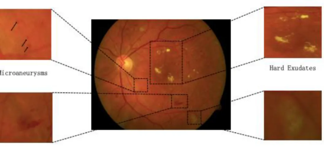
The physicians have laid out the stages of DR by pointing out the symptoms. A sample retinal image with the manually annotated common DR lesions [14] is shown in Figure 1.

5 The typical lesions of DR are briefly discussed below:

 Hard Exudates: Hard exudates are one of the retinal lesions that define DR. Hard exudates usually appear in the retinal images as tiny yellow-white spots with sharp edges and different sizes [15].

 Soft Exudates: Soft exudates, also known as cotton wool spots, appear as white patches with blurred and hazy edges [16]. Exudates, including soft exudates and hard exudates, are one of the most common early lesions of DR [17].

 Microaneurysms: Microaneurysms are the earliest clinically visible signs of non-proliferative diabetic retinopathy (NPDR) and are caused by dilatations of thin blood vessels. Microaneurysms usually appear as small red dots with sharp edges (20 to 200 microns) in clusters [18].

 Haemmorhges: As microaneurysms rupture in the deeper layers of the retina, they form hemorrhages.

In the United Kingdom (UK), the National Health System (NHS) is the publicly funded healthcare system and they have laid out the Diabetic Eye Screening Programme (DESP) According to them, for grading the retinal fundus images usually up to three human graders are required. These graders must meet the NHS DESP quality assurance standards and should be able to assess the images to determine a disease severity grade. They should then use these grades to produce a ‘final grade’ for each eye according to the highest level of severity observed. The stages of DR can be classified based on the presence of clinical features. The four widely used DR levels are defined in the table below [19] in Table 1.

6 Table 1. Stages of DR [19].

Figure 2. Stages of DR - UK equivalence for Diabetic retinopathy stages [20].

Figure 2 shows the various stages of Diabetic Retinopathy and the UK equivalence scale. The normal fundus equates to R0. The stage characterized by microaneurysms only is the Mild non-proliferative DR stage and the next stage where there are distortions in the blood vessels surrounding the retina causing swelling and degradation in the ability of blood transportation. Both mild and moderate non-proliferative DR equate to R1 in the UK equivalence scheme. Severe Non-non-proliferative DR are characterized to the blockage of more blood vessels and are depicted by more than 20 intra retinal hemorrhages in each quadrant along with venous beading. It equates to R2 in UK equivalence standards. Proliferative Diabetic retinopathy is

Levels Description

R0 No DR

R1 Presence of Microaneurysms, retinal hemorrhages and any exudates R2 Presence of Intra-retinal microvascular abnormalities, venous loop,

venous beading

R3 Presence of new blood vessels (neovascularization), pre-retinal or vitreous hemorrhage

7 characterized by vitreous hemorrhage and/or Neovascularization (new blood vessels formation) which are prone to bleed and leak more often. They equate to R3 stage in the UK equivalence standards [21] [22].

1.1.3 Fundus Photography

Color Fundus Retinal Photography which is widely used for screening the retina of patients uses a fundus camera to record the conditions of the eye focusing a 3D eye retina structure into a 2D plane. They record color images of the retina. The camera is basically a microscope with low power and has a camera attached to photograph the interior of the eye. The camera can clearly picturize the internal retinal features including the retinal vasculature, optic disc, macula, etc. The image is formed by the amount of light reflected by the interior of the eye. The imaging light is sent to the retina via the pupil to form the image by the reflected rays from the retina (Figure 3).

Figure 3. The scope of fundus imaging [32].

Lack of appropriate intervention causes DR to progress from mild to severe stages and thus it is important to recognize the stages when referral for treatment may be most beneficial. DR is broadly classified into two categories: non-proliferative

8 diabetic retinopathy (NPDR) and proliferative diabetic retinopathy (PDR). Management of NPDR involves close monitoring by an ophthalmologist or optometrist and optimization of the patient’s glycemic control by an internist. Treatment at the proliferative stages involves laser photocoagulation, intravitreal injections of anti-vascular endothelial growth factor (VEGF) agents, or surgery to repair a retinal detachment.

1.2 Motivation

DR is a major cause of blindness and manual diagnosis of DR from retinal images is a time-consuming process and cumbersome process. Further it requires expertise of trained healthcare professionals which are often scarce, thus making it a challenging process. As a result, several studies have used deep CNN models to diagnose DR automatically. However, these methods employed very deep CNN models (e.g., ResNet-based method [23], Inception Net-based method [24], InceptionNet-ResNet-based model [25]) which require vast computational resources. Research on DR screening using computationally efficient CNN models has a great practical significance. This thesis is therefore focused on applying accurate and computationally efficient CNN model of MobileNetV2 for automatic DR classification that h can be deployed in mobile environments with scare resources like memory and computation power.

1.3 Research Questions In this research we aim to research the following questions:

 Can lightweight architectures like MobileNetV2 effectively classify the severity of DR using retinal images and give comparable results to the commonly used heavy and dense architectures like DenseNet, VGG etc. using transfer learning?

9

 Can transfer learning model built using MobileNetV2 architecture give a good performance using a custom dataset of handpicked retinal fundus images employing various image processing and finetuning techniques?

 Does the developed model give satisfactory results when compared to other related work in the literature and does it hold a good scope of deploying in real-time mobile applications for clinal testing?

1.4 Research Aims and Objectives

The aim of this research is to classify the severity of Diabetic Retinopathy (DR) using retinal fundus images using light weight mobile networks.

The Objectives are as below:

1. To compare the performance of models built using light weight mobile networks like MobileNetV2 with the commonly used heavy and dense transfer learning algorithms on retinal fundus images.

2. To train and test a lightweight mobile-friendly classifier using MobileNetV2, using a custom-made dataset which can be deployed in mobile-based screening systems to classify the severity of DR.

3. To compare the developed model with existing work in the literature and assess the scope of real time deployment of the model in a mobile environment for testing in a clinical setting.

Summary

In this chapter we have laid forth the foundations of the study, the problem, the motivations behind the study, giving an overview of Diabetic Retinopathy and the various stages and classifications used in the medical community. We further put down the objectives of the study which has been described further in the following chapters.

10 CHAPTER 2: BACKGROUND

This chapter is a brief overview of various necessary background concepts that are needed to understand the contents of the thesis. The chapter highlights the concept of Artificial Intelligence (AI), the basic intuition of Machine Learning (ML), foundations of Deep Learning and its relationship to ML. Further, we explain the Convolution Neural Networks (CNNs) which are popularly used in the field of Computer Vision. We further understand the architectures of the CNNs which were used in this thesis. We also understand the intuition behind transfer learning and how we have leveraged it for our experiments. We also present the structure of the light weight, computationally efficient MobileNetV2 architecture.

2.1 Artificial Intelligence

Artificial Intelligence (AI) is a field of computer science where the machines demonstrate intelligence just like the natural intelligence displayed by humans and animals. AI research has seen a resurgence, following the phase of AI winter, after being founded in 1955, as an academic discipline. This was mostly due to the availability of large amounts of computational power, the enormous amounts of data and the theoretical understanding that was necessary to simulate the human intelligence. The field of AI includes many subfields like knowledge representation, reasoning, learning, planning, natural language processing, perception and the ability to move and manipulate objects. Automated reasoning is an area which involves knowledge representation and reasoning to help computers acquire the ability of reasoning. Natural language Processing deals with the development of computers ability to process large amounts of natural language data and analyze it. Machine perception deals with developing the ability of the computer to absorb the sensory inputs and be able to see, feel and perceive the way humans do by gathering information

11 from the world using machine vision, hearing and touch. Fields of computer vision, machine hearing and machine touch fall under this category. Hence, learning which is formally termed as Machine Learning (ML) is a subset of AI where the machine learns from data by identifying patterns in the data and forming inferences using several algorithms and statistical techniques.

2.2 Machine Learning

It is a subset of AI which allows the machine to learn from data implicitly without being actually programmed. The machine learns from the data by identifying patterns and making predictions. The popular machine learning algorithms include, the decision tree, k-nearest neighbors, naïve bayes, neural networks and kernel methods like support vector machines (SVMs). The task of these learning algorithms is to learn from data. In machine learning the algorithms essentially learns from an experience E with respect to some class of tasks T and performance measure P, if its performance at tasks in T, as measured by P, improves with experience E [70]. Examples of these tasks are classification, regression, anomaly detection etc. Examples of the performance measure P is accuracy, error rate etc. Examples of the learning experience are supervised, unsupervised and reinforcement. The learning experience basically denotes the type of learning that the algorithms are allowed to have during the learning process. In supervised learning experience the algorithm has a dataset which has labels while unsupervised learning experiences are based on data which don’t have labels. Reinforcement learning experience deals with the model learning from the environment through feedback loops. A dataset is a collection of examples which is in turn a collection of features. The entire collection of steps that make up the ML pipeline include data collection, data cleaning, splitting the dataset into training, validation and testing data, feature selection and engineering, model building, hyperparameter tuning,

12 and model optimization.

2.3 Deep Learning

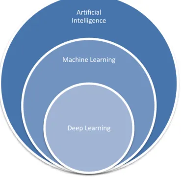
Deep Learning is a subset of Machine Learning which comprises of architectures that use Deep Neural Networks (DNN). Figure 4. depicts the relationship of Artificial Intelligence, Machine Learning and Deep Learning.

Figure 4. Relationship between AI, ML and DL.

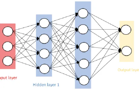
Deep Neural Networks trace their origins back to the 1940s and 1950s and are inspired by the biological neural networks of the brain [26]. A typical neural network consists of 3 layers called input layer, the hidden layers and the output layers. The input layer takes the input from the data and passes it to the hidden layers which perform a non-linear combination of the information from the previous (input or hidden) layers. All these layers are composed of a neuron which is similar to structure of the biological neuron of the human brain. The building block of a neural network is a neuron which

Artificial Intelligence

Machine Learning

13 is depicted in the figure 5.

Figure 5. The basic structure of a neural network.

.

14 A neuron (Figure 6) is basically a placeholder for a mathematical function called as the activation function which activates this neuron by specific degrees based on the inputs and fires and output. Each layer of a neural network is a collection of neurons which take inputs and provide an output. The neural network in figure 4 has an input layer which takes the input and feeds it forward to the hidden layers which are activated based on the specific activation functions and which then produce an output based on their activations. The parameters are the weights, denoted by w (also a [nx1] vector), and a bias scalar, denoted by b. An activation, denoted by a, is a scalar defined by:

A point-wise non-linear function, denoted by σ (·), is then applied to generate the output, y = f(a) = σ( ∑𝑛_𝑖=1𝑥𝑖𝑤𝑖 + b). Some choices for the non-linearity function σ includes, sigmoid function, Tanh function, ReLU or the Leaky ReLU.

Other terminology used in the literature for this type of structure includes Artificial Neural Networks (ANN), Multi-layer Perceptron (MLP), and a fully-connected network. By convention, the number of layers is equal to the number of hidden layers plus the output layer (i.e., excludes the input layer).

Once a model architecture has been selected, the next step is to train the model as denoted by the steps below:

 Given the dataset of input x and output y, pick an appropriate cost function, C.

 Forward pass the input examples through the model to arrive at the predictions. Here the neurons are fired based on the activation’s functions.

 Calculate the error using the cost function C to compare the predictions.

 Apply back-propagation to pass the error back through the model, adjusting the parameters to minimize the loss L.

15

 Once the gradients are established, use Stochastic Gradient Descent (SGD) to update the network weights.

In SGD, we start with some initial set of parameters, denoted by θ0_{, and the updates} are defined by θ k+1 _{← θ} k _{+ η ∆θ, where k is an iteration index, η is the learning rate,} and the gradients ∆θ = ∂ L /∂ θ.

The backpropagation algorithm involves:

1. A forward pass where for each training example we compute the output for all the layers, xi = Fi (xi−1, wi);

2. A backwards pass where we compute cost derivatives iteratively from top to bottom ∂C/∂xi−1 = ∂C/ ∂xi · ∂Fi (xi−1, wi) / ∂xi−1

3. Compute gradients and update the weights.

A constant learning rate η is typically not optimal. Techniques to optimize the learning rate are AdaGrad, RMSProp and ADAM. A momemtum term can be added to the weight update to encourage updates to follow the previous direction. This usually helps speed up convergence. The update then become θ k+1 ← θ k + α(∆θ) k−1 – η ∆θ, where α is typically around 0.9.

2.3.1 Convolutional Neural Networks

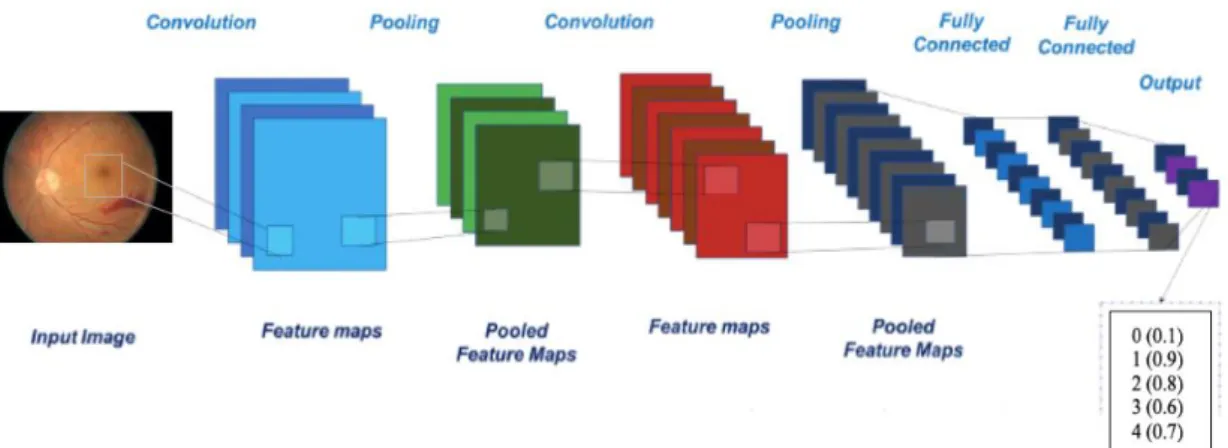
A popular class of Neural Networks are the Convolution Neural Networks (CNNs) which have shown exceptional performance in the field of image classification and recognition. The CNN network architecture has a number of hidden layers which help in the extraction of useful features and a fully connected layer at the end used for the classification. The CNN model is feed-forward, where input images are fed to convolution layer(s), non-linearities, pooling layers, and finally to feature maps. The CNN architecture, as shown in Figure 7, comprises of alternating convolution and pooling operation to reduce computation time and to understand the spatial details more

16 effectively [27] [28] [29].

Figure 7. A convolution neural network.

The optimization process of the network is done by the backpropagation algorithm and the stochastic gradient descent algorithm. The convolutional layers apply a convolution operation with a fixed sized filter, e.g. 3x3 or 5x5, across the image. The filter is learned during training, and options such as the stride, padding, and dilation can be set. The pooling layer helps to reduce the spatial size of the representation, thus reducing the number of parameters and computation, and to prevent overfitting.

ImageNet [69] is a large-scale image database with over 14 million labeled images and over 20K classes. The ImageNet Large Scale Visual Recognition Challenge (ILSVRC) is an annual competition, where teams compete to build high performing networks. In 2012 major breakthrough was achieved via the AlexNet CNN of Krizhevsky et al. [30], achieving a top-1 and top-5 error rates of 39.7% and 18.9% which was considerably better than the previous state-of-the-art results.

2.3.1.1 DenseNet161 architecture

DenseNet (Densely Connected Convolutional Networks) is one of the latest neural networks for visual object recognition [35]. It’s considerably similar to ResNet

17 [34] but has some fundamental differences. It addresses the issue of “vanishing gradients”. Specifically, the DenseNet authors point out that with increasingly deep CNNs as information about the input or gradient passes through many layers, it can vanish and “wash out” by the time it reaches the end (or beginning) of the network. ResNet architecture proposed Residual connection, from previous layers to the current one. This is exactly how the DenseNet layers deal with this issue. DenseNet created an architecture to ensure maximum information flow between layers in the network, by connecting all layers (with matching feature-map sizes) directly with each other. In contrast to ResNet, DenseNet never combines features through summation before they are passed into a layer, rather it combines features by concatenating them. The “denseness” occurs because this network introduces L(L+1) 2 connections in an L-layer network, instead of just L in traditional architectures [35]. Figure 8 depicts a 5-layer dense block with a growth rate of k = 4. Each layer takes all preceding feature maps as input.

18 Figure 8. Schematic diagram of DenseNet architecture, reproduced from [35].

The biggest advantage of DenseNets is the improved flow of information and gradients throughout the network as each layer has direct access to the gradients from the loss function and the original input signal, leading to an implicit deep supervision.

2.3.1.2 VGG16 architecture

VGG16 is a deep CNN used for object recognition which was developed and trained by Oxford's renowned Visual Geometry Group (VGG) and gave 92.7% top-5 test accuracy in ImageNet in the Large-Scale Visual Recognition Challenge 2014 (ILSVRC2014) [33]. ImageNet is a huge database of images for academic researchers with 14 million hand-annotated images of what is in the picture. The main contribution of VGG is to show that classification/localization accuracy can be improved by increasing the depth of CNN in spite of using small receptive fields in the layers. (especially earlier layers). Neural networks prior to VGG used bigger receptive fields (7*7 and 11*11) as compared to 3*3 in VGG, but they were not as deep as VGG. There are few variants of VGG, the deepest one is with 19 weight layers. In this research, the

19 model with 16 layers has been used which is popularly known as VGG-16.

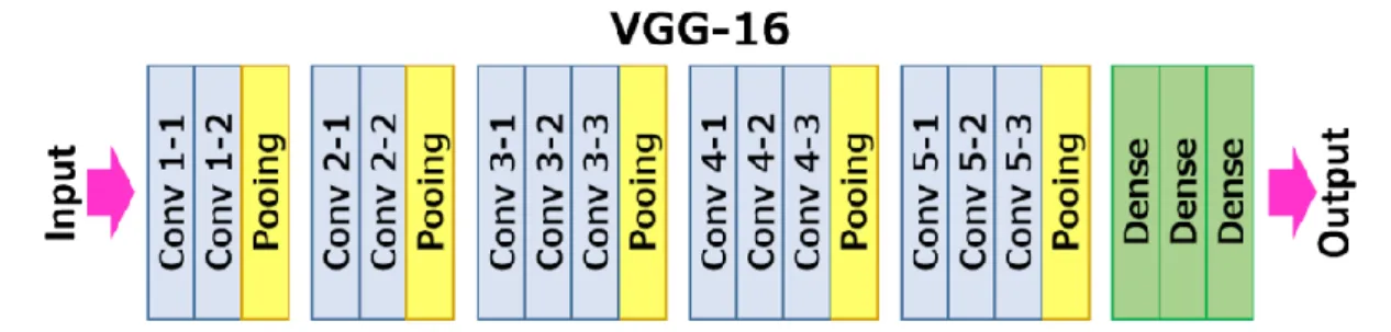
VGG-16 is named so as it has 16 layers as shown in figure 9. It consists of Convolutional layers, Max Pooling layers, Activation layers, Fully connected layers arranged together as shown in figure 9 below which gives an overview of the layers in a VGG-16 network.

Figure 9. VGG-16 Layer Architecture.

There are 13 convolutional layers in the VGG-16 network, 5 Max Pooling layers to down sample the size of the network and 3 Dense layers which sums up to 21 layers but since only 16 weight layers, are there the network is named as VGG-16.

2.3.1.3 MobileNetV2 architecture

Transfer learning using Image net weights on MobileNetV2 has been taken into consideration for this thesis as this network is the state-of-the-art approach in the most mobile compatible networks. The biggest drawback of the commonly used CNNs such as DenseNets and VGG etc. is that they are computationally expensive. MobileNets are neural networks which are very efficient for mobile devices. MobileNetV2 is an enhancement of MobileNetV1 and is much more efficient and powerful than its predecessor. The original MobileNetV1 is a CNN which uses depthwise separable convolutions and basically splits the convolution layer into two sub tasks i.e. The input

20 is filtered by a depthwise convolution layer and then a pointwise convolution of size 1x1 combines these filtered values to create new features. These two layers are together termed as ‘depthwise separable convolution block’ which performs the tasks of a normal CNN but much faster, almost about 9 times as fast as other neural networks giving about the same accuracy [11]. The structure of the MobileNetV1 has these layers followed batch normalization and the ReLU6 activation function is used which is known to give better performance than the regular ReLU. At the end, there is a global average pooling layer, followed by a fully connected layer or a 1x1 convolution, and a softmax. The depth multiplier which is also known as the width multiplier is a hyperparameter which can be tuned and controls the number of channels in each layer [8].

Table 2. Depthwise Separable vs Full Convolution MobileNet reproduced from [8] on ImageNet dataset.

Network ImageNet Accuracy Million Mult-Adds Million Parameters

Conv MobileNet 71.7% 4866 29.3

MobileNet 70.6% 569 4.2

Table 2 clearly demonstrates the effect of depth wise separable convolutional layer. Conv MobileNet, which uses the standard convolutional layer gives an accuracy of 71.7% while MobileNet which is based on the depth wise separable convolutional layers gives an accuracy of 70.6%, when trained on the ImageNet dataset. Additionally, the Mult-Adds operations and the learnable parameters are reduced significantly due to the depth wise separable layer. Hence significant improvement in the efficiency is

21 observed by reducing the parameters and Mult-Adds significantly while trading off the accuracy only by approximately 1%. This explains the contribution of depthwise separable layer which make up the MobileNet architecture, thus making them highly efficient for mobile devices.

According to Sandler et.al. [9] MobileNetV2 s similar to MobileNetV1, with differences in the architecture which contribute to its effectiveness. It also uses depthwise separable convolutions but the structure of the building block has residual skip connections and the expansion and projection layers, in addition. The building block consists of three convolution layers i.e. an expansion layer in which a 1x1 convolution layer expands the number of channels, a second layer which called the depthwise convolution layer and filters the inputs, followed by a third layer which is called the projection layer (and is a 1x1 pointwise convolution) which makes the number of channels smaller [9]. The expansion factor gives the factor by which the data gets expanded in the expansion layer and is a hyperparameter with a default value of 6. The network also has residual connections which helps with the flow of gradients through the network. Similar to MobileNetV1, every layer has batch normalization and the activation function is ReLU6 but the output of the projection layer in MobileNetV2 does not have an activation function applied to it. The complete MobileNetV2 architecture consists of 17 such building blocks followed by a regular 1×1 convolution, and a global average pooling layer, and a classification layer which is a 1x1x N layer where N is the number of classes in our problem [9].

Sandler et.al. mention that MobileNetV2 performs 300 million MACs which are the multiply-accumulate operations for an RGB image of 224x224, while MobileNetV1 performs 569 million MACs [12]. Additionally, V2 has nearly 20% less

22 parameter counts than V1 has and this explains why V2’s is more computationally efficient that V1 for mobile devices which have low memory access and less computation power [9].

Sandler et al. [9] termed the 2 building blocks as the inverted residual building block with linear bottlenecks which is fact the expansion layer and the reduction building block with linear bottlenecks which is the projection layer. Table 3 shows the architecture of the MobileNetV2 network and figure 10 shows the building blocks of the network. Similar to MobileNetV1 architecture, a hyperparameter α is introduced to trade off performance and computational cost. It is found that MobileNetV2 achieves an Accuracy of 0.720 compared to an Accuracy of 0.706 achieved by MobileNetV1 while using 19% fewer parameters and 48% fewer MAdds on ImageNet dataset [9].

Figure 10. Inverted Residual (left) and Linear Bottleneck (right), Convolution blocks of MobileNetV2 reproduced from [9].

23 Table 3. MobileNetV2 vs MobileNetV1 reproduced from [9] on ImageNet dataset.

Network ImageNet Accuracy Million Mult-Adds Million Parameters

MobileNetV1 70.6% 575 4.2

MobileNetV2 72.0% 300 3.4

2.4 Transfer Learning using Convolution Neural Networks

Transfer learning is a technique developed to address the issue of applying deep learning for domains with limited data [31]. The basic idea is to leverage the fundamental learning blocks built with a particular Deep Neural Network (DNN), such as ResNet, and to “re-train” the DNN for a particular domain of interest. Thus, one can utilize the strong “fixed feature extractor” capabilities of a DNN built on the millions of training examples from ImageNet to detect features common to all domains, such as object edges, and then re-train just the “top layer” for classification with the limited training data from a particular target domain.

Transfer Learning reduces the training time significantly. It also reduces the size of the dataset used for learning and this makes it very useful in domains which have little data. Training the final layers means that we transfer the knowledge that the classifiers learned from the its original training and can now apply it the smaller dataset from a different domain without the need for extensive training, thus saving training time and computational resources, and building models which give accurate results.

In this study, we have tried experimenting with the famous DenseNet121, VGG16, and MobileNetV2. We have tried to classify retinal images into respective categories using the original pretrained network which was trained on image net weights and we modified those networks by removing the top classification layers and by replacing them with pooling layers, dense layers and the final classification layer of

24 5 x1 nodes for the 5 output classes. This section of the overview of deep learning will briefly review 3 DNNs that were evaluated in this report. These networks are DenseNet121, VGG16, and the lightweight MobileNetV2.

Summary

In this chapter we have discussed in detail the basics behind the deep neural networks, the feed-forward process and the backpropagation algorithm which is used to update the weights learned from the input. We have also looked at Convolution Neural Networks and have discussed the various CNN architectures used in this thesis. The following chapter presents the related work done in the field of DR severity grading using artificial intelligence.

25 CHAPTER 3: RELATED WORK

In this chapter we present the related work highlighting key studies which have worked on the problem of diabetic retinopathy grading using computerized approach. We will study the various techniques and approaches used by the previous studies and how our study stands out from them.

3.1 Related work on DR screening

DR screening is based on retinal examinations by trained ophthalmologist or optometrist, or by digital retinal images which can detect early stages of DR. [36]-[44]. Manual screening for DR using digital imaging is known to give satisfactory results, however with the rise in DR prevalence coupled with the limited number of trained eye care professionals or certified readers, current DR screening programs that rely on expensive labor-intensive manual assessment may fail to address the rising screening demand, especially in the rural or non-developed nations which lack access to qualified screeners. To address such issues two alternative methods, exist in the literature i.e. crowdsourcing and automated computer aided retinal image analysis. The following sections gives some insights into the methods.

3.1.1 Crowdsourcing

Amazon’s Mechanical Turk (AMT) is a crowdsourcing platform which lets us hire remote workers to do specific jobs which computers may be unable to do. One study [45] used Amazon Mechanical Turk to find an accuracy of 81.3% for distinguishing between normal and abnormal images while another study [46] found an accuracy of greater than 90% in distinguishing normal and severely abnormal images. Both the studies indicated a sensitivity of greater than 93% indicating that this screening modality has a good potential to address the increasing volume of images that will need to be screened with increasing diabetes prevalence rates. However, this technique has

26 its obvious limitations i.e. there is no control over who is the “the crowd” in such platforms as it is counter to the spirit of crowdsourcing, but in reality, it is indeed necessary to know and have control over who is performing the analysis to validate the quality of image analysis [47].

3.1.2 Computer-aided retinal image Analysis

There is a plethora of studies which are focused on DR grading via automated mechanisms based on machine learning algorithms. The studies can be grouped into two very broad categories i.e. one which uses traditional approaches and the other which follow end to end methods.

3.1.2.1 DR Screening Using Traditional Methods

The traditional methods comprise of different phases which are distinct and separate. The phases usually are (1) feature extraction, (2) training and (3) classification/grading. The feature extraction phase depends on one or more of the DR symptoms. Usually the target is to extract the features of DR such as changes in the blood vessels which usually requires blood vessel segmentation and/or detection of lesion and classification which includes exudates, microaneurysms, hemorrhages, etc. For example, Nijalingappa and Sandeep [2] used traditional techniques to detect Microaneurysm in digital fundus images on a local dataset and achieved an accuracy of 87%. Microaneurysms are localized capillary dilations in circular shape and appear like small red dots often in clusters. Similarly, Seoud et al. [48] conducted experiments for detecting red lesions (i.e., Microaneurysm and Hemorrhages) in 2016 and achieved a sensitivity of 96%. They built a traditional model based on both Random Forests and Decision Trees algorithms.

In [49], Support Vector Machines (SVMs) have been used to detect and classify the exudates and predict the severity of DR. In the research conducted by Acharya et

27 al, an automated system was developed for identifying the five classes using the features extracted. Some studies [50], [51] extracted exudates as features to classify the retinal images while some others used number of microaneurysms [52] while some other studies focused on retinal blood vessels [53] to identify diabetic retinopathy. Hence within the literature there are various trends and techniques to classify the severity of diabetic retinopathy and these techniques are heavily varied.

There is variation in the type of image processing techniques used as well. Rakshitha et al. [54] used several image transformation methods to enhance the images. She used contourlet transform, curvelet transform and wavelet transform and compared the performances of the classifiers. Another study [55] experimented with discriminant texture features to detect diabetic retinopathy. Most of these image processing techniques aim at identifying the lesions (exudates, hemorrhages, microaneurysms etc.) and the blood vessels to detect diabetic retinopathy.

Medical doctors and/or domain experts are required to put in their expert knowledge in the case of feature-based classification methods. This process of feature selection and extraction manually is often time consuming and varies vastly. Current trends in the literature point towards the DL based systems which use CNN’S. these models have been able to outperform the traditional approaches which use extraction of features. Hence end to end methods which primarily use the state-of-the-art deep learning models depend on pixel locations, correlations between the pixels, the color intensities and/or the combination of these features to create more sophisticated features. Over the last few years this step led to the automation of the feature extraction phase without any manual investigation or selection of the features. CNNs have demonstrated encouraging results in both the identification and grading of DR symptoms. Deep Learning algorithms are mainly used for classification based either

28 from scratch or for transfer learning.

3.1.2.2 DR Screening Using Deep Learning & Transfer Learning technique

Transfer learning uses the technique of transferring the weights from a pre-trained model to adjust to our learning dataset. Maninis et al. [56] used VGG-16 for transfer learning for optic disk and blood vessel segmentation and achieved good results. Mohammadian et al. [57] used the Inception-V3 algorithm and fine-tuned the parameters and also used the Xception pre-trained models and achieved promising results. In addition to balancing the dataset they used data augmentation techniques and achieved an accuracy of 87.12% using Inception-v3 algorithm.

The study published in [58] demonstrated how transfer learning could solve the issue of insufficient training data. The authors in this paper use transfer learning for retinal vessel segmentation. Along similar lines studies like [59] and [60] used transfer learning and in [60] the best model was developed using VggNet-16 which achieved a 78.3% accuracy. Hence, we see a number of recent studies are targeting transfer learning to solve the inadequacy of data in the domain and also reducing the training time.

With the increase in smartphone usage, smartphone-based Point-Of-Care-Technology (POCT) is becoming popular. Rajalakshmi et. al. [5] and Xu et. al. [61] in two separate studies have used smartphone-based applications coupled with a fundus camera hardware for diabetic retinopathy grading. We lay forth the foundations of our study based on the related literature existing in the domain.

3.1.2.3 DR screening using MobileNetV2

MobileNetV2 is similar to MobileNetV1, with differences in the architecture which contribute to its effectiveness. It also uses depth wise separable convolutions, like its predecessor but the structure of the building block has residual connections and

29 the expansion and projection layers, in addition. MobileNetV1 are a neural network architecture which are very efficient for mobile devices. MobileNetV2 is an enhancement of MobileNetV1 and is extremely powerful for mobile devices which are targeting models which give low latency and high computational efficiency.

In [62] the authors experimented with MobileNet and MobileNetV2 among other transfer learning approaches on the problem of diabetic retinopathy grading. They used MobileNetV2 which is an improvement of the MobileNetV1 architecture in terms of speed and computational efficiency and also gave good performance. They achieved an accuracy of 78.1% using MobileNetV2 and an accuracy of 58.3% using MobileNetV1.

Further, we see that Gao et.al. in [63] divided the problem into a 2-class problem of DR and RDR which is referable DR. According to them, grade 0 and 1 of the Messidor dataset form the DR category while grade 2 and 3 are considered the referable DR category which needs urgent attention. Their MobileNetV2 model has achieved an accuracy of 90.8% for class DR and 92.3% for class RDR [63]. Due to a difference in the annotation scales used in the datasets Gao et.al. [63] transformed the problem into a binary classification task of referable vs non- referable.

To the best of our knowledge no other study has first validated the performance of pre-trained DNNs on retinal fundus image and then built a custom dataset of handpicked images to build a light weight mobile friendly model using MobileNetV2 to classify retinal images for DR retinal screening. In this study, we used a custom-made dataset of handpicked retinal fundus images from 3 different publicly available datasets and then trained and tested our classifier using MobileNetV2 on these images after using several preprocessing techniques. In this study we present the methodology

30 and the results of applying transfer learning algorithms to retinal fundus datasets and then using MobileNetV2 on a custom dataset to fine tune the model and build models specifically for the needs of mobile devices which has the potential to be used for screening DR using mobile devices.

Summary

In this chapter we have analyzed the various studies in the literature which have done similar work and laid forth the methodology used in our study in the next chapter. We have tried to cover the broad areas where automated diabetic retinopathy severity classification was being carried out. The nest chapter will explain the methodology followed in this research.

31 CHAPTER 4: METHODOLOGY

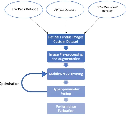
In this chapter we lay forth the foundations of the research by explaining the dataset used in the study, the architecture of our model, the preprocessing techniques and the hyperparameter tuning that was done to achieve the optimal performance. Figure 11 and Figure 12 explain the methodology diagrammatically.

Figure 11. Diagrammatic overview of the methodology – Part 1.

4.1 Datasets

For the first part of our study we trained our models using pretrained networks on a publicly available Diabetic retinopathy dataset from Kaggle i.e. the APTOS 2019 Blindness Detection dataset from Kaggle [64]. The dataset comprised of retinal fundus images which were split first into train and validation where 10% of the data was randomly chosen for validation. The train data was split into training and testing data using train_test_split from sklearn with the test_size being 15% of the remaining data. The dataset has retinal fundus images which are rated by a clinician for the presence of diabetic retinopathy in each image on a scale of 0 to 4. The five classes are as follows:

32

0 - Negative or No DR: Patient has no disease.

1 - Mild DR (Stage 1): Patient has mild level of disease.

2 - Moderate DR (Stage 2): Patient has moderate level of disease.

3 - Severe DR (Stage 3): Patient has severe level of disease, the most part of the retina is damaged, can lead to complete blindness.

4 - Proliferative DR (Stage 4): Patient has proliferative level of disease. The patient’s eye is damaged to an extent where treatment is elusive, about 80 percent of blindness exists.

Further in order to build an accurate, computationally efficient and robust system, we prepared a custom dataset using 3 different publicly available datasets to train and test our model using the light-weight MobileNetV2 architecture. The final dataset that we used in our experiments is an amalgamation of retinal fundus images from the three datasets mentioned below:

1. EyePacs dataset: EyePacs has provided a large dataset of retinal images from diabetic screening programmes [65]. The dataset is sponsored by the California Health care Foundation and was used in the Kaggle DR Detection Challenge. This dataset comprises a large set of high-resolution retina images taken under a variety of imaging conditions. It has a total of 88,702 JPEG images. The competition sponsors pre-allocated 31,615 (35.6%) of these images for training, 3,511 (4.0%) for validation, and 53,576 (60.4%) for testing. Class labels were provided by the competition for the training, validation, and test images. The dataset is labelled with a severity grade of DR from 0 to 4. All images were rated by a certified reader according to a standard diabetic retinopathy grading scale.

2. APTOS 2019 dataset: APTOS stands for Asia Pacific Tele-Ophthalmology Society [64]. It is a subset of the EyePacs dataset obtained after performing some

33 preliminary operations and available in different image formats. It consists of 3000+ images.

3. Messidor 2 dataset: The Messidor 2 is an extension of the original Messidor dataset for diabetic retinopathy [66]. It contains 1500+ retinal fundus images which are labelled with 4 classes from 0 to 4.

We performed data normalization on images from the 3 datasets in a way that each of the 5 classes has relatively the same number of images. This was done to ensure that the dataset is not biased towards any one particular class. We used partial datasets from EyePacs and APTOS 2019 dataset and used 50% of the Messidor2 dataset to create this custom dataset for training our classifier in our experiments and we only choose images which were of a good quality and would contribute good features to the classifiers. The other 50% of Messidor2 dataset was kept aside and was used for testing the performance of our classifier. The testing dataset has 961 images belonging to the 5 classes, explained above.

4.2 Image Pre-processing and Augmentations

For testing the performance of the 3 classifiers we experimented with a few preprocessing techniques. For each image we have applied the following transformations i.e. horizontally flip 50% of all images, vertically flip 20% of all images, scaled images to 80-120% of their size, individually per axis, translated by -20 to +20 percent (per axis), rotated by -45 to +45 degrees, shear by -16 to +16 degrees, used nearest neighbor or bilinear interpolation (fast). We further converted images into their super pixel representation and blurred the images with a sigma between 0 and 3.0. We add further processing by blurring the image using local means and medians with kernel sizes between 2 and 7. We added gaussian noise to the images and randomly remove up to 10% of the pixels. We experimented with using inverted color channels

34 and changed the brightness of the images (by -10 to 10 of original value) and also with changing the hue and saturation. We have also removed any ovals from the dataset and kept only the circular ones so that we can remove any bias and train the algorithms with images where every image contributes equally to the learning process. We used these transformations on the images based on our literature survey that we conducted and chose the techniques which gave promising results.

Figure 12. Diagrammatic overview of the methodology – Part 2.

Further when we worked on building a lightweight mobile friendly MobileNetV2 model which gave promising results. We employed certain image

35 preprocessing techniques to improve the quality of the images. We changed the luminous intensity of the image which altered the brightness and made the details of the image more visible. We considered changing alpha, beta and gamma channels which are the important channels which control the amount of the light. We checked for images which were too dark or over-bright and could be augmented by altering the alpha, beta and gamma channels and controlled the light by using alpha = 2.5, beta = 40 and gamma = 1.44. These values were obtained using trial and error method on several dim images using OpenCV’s ConvertscaleAbs function [67].

In order to transform the image to perform texture analysis with an enhanced signal to noise ratio and provide better luminance ranges to the input images we used OpenCV’s Bioinspired_retina functionon some of the retrieved dim images andthen augmented some particular parameters [68]. This function helps in performing texture analysis and improves the signal to noise ratio. We particularly altered the default values of the following parameters in the function using retina configurations:

 photoreceptorsLocalAdaptationSensitivity: 0.69  photoreceptorsTemporalConstant: 8.9999997615814209e-01  photoreceptorsSpatialConstant: 5.2999997138977051e-01  horizontalCellsGain: 0.75  hcellsSpatialConstant: 7.0  ganglionCellsSensitivity: 0.75

These preprocessing steps helped us in bringing up enriched features from the images, following which, we applied data augmentation using horizontal and vertical flips and rotation using -20 to +20-degree rotation. We were able to bring 3400+ images in each class with a total of 17,121 images in the final dataset. 80 % of the images were used for training, and 20 % were used for validation. We tested the performance of the

36 dataset on unseen data, which was 50% of the messidor2 dataset kept aside specifically for this purpose.

4.3 Model Architecture and Training

We compared 2-different models for our experimentation which were heavily used in the literature i.e. DenseNet121, VGG16 and a light weight MobileNetV2. We used pretrained weights on ImageNet dataset. The last layer was modified and we introduced Global Average Pooling (GAP layers). This was done to reduce the total number of parameters and thus reduce overfitting. The GAP layers are used to reduce the spatial dimensions of a 3-d tensor just like the Max pooling layers. And then Dropout with 0.5 as regularizer. During training we freeze the first layers and trained the last 4 layers including classifier for transfer learning. Feature extractor was trained on ImageNet. These experiments were conducted with an intuition to compare the performance of the lightweight architecture of MobilenetV2 with the other heavy and dense architectures and record their results. Architecture of one of the transfer learning algorithms - the DenseNet121 is depicted in Figure 13 below.

Since the aim of the study was to build a light weight mobile friendly architecture using MobileNetV2, transfer learning using Image net weights on MobileNetV2 has be taken into consideration in this work as this is the state-of-the-art approach in the most mobile compatible networks. MobileNetsV1 are a neural network architecture which are very efficient for mobile devices. MobileNetV2 is an enhancement of MobileNetV1 and is much more efficient and powerful than its predecessor. According to Sandler et.al. [9] MobileNetV2 is similar to MobileNetV1, with differences in the architecture which contribute to its effectiveness which have been explained in Chapter 2 (section 2.2.3). The structure of our final model tested on the custom dataset is given in Table 4.

37 Figure 13. Schematic representation of Classification with DenseNet121.

Table 4. The structure of MobileNetV2 architecture used for DR Classification. Input Dimension Operator

t c n S 2242 x 3 Conv2D - 48 1 2 1122 _{x 48 Residual Module 1 24 1 1} 1122 x 24 Residual Module 6 32 2 2 562 x 32 Residual Module 6 48 3 2 282 _{x 48 Residual Module 6 88 4 2} 142 x 88 Residual Module 6 136 3 1 142 x 136 Residual Module 6 224 3 2 72 _{x 224 Residual Module 6 448 1 1} 72 x 448 Conv2D 1x1 - 1792 1 1 72 x 1792 AvgPool 7x7 - - 1 - 12 _{x 1024 Dense 1 1024 2 1} 12 x 512 Dense 1 512 1 1 12 x 5 Dense - Final 1 5 1 -

38 4.4 Training and Hyperparameter tuning

We trained our final model on the custom dataset and validated its performance using the validation set. The 80% of our custom dataset was used as training set and the other 20% was used for validation.

We chose a learning rate of 0.00015 where the network converged faster. We used Adam with AMSGrad as our optimizer after trying several other optimizers and used a batch size of 32 for CPU training. We used a Dropout of 0.1. We ran a grid search on number of unfreezing layers and found that when we unfreeze half of the MobileNetV2 layers the model accuracy is more and the learning is very fast and the model converges very fast.

We freezed the first 80 layers and unfreezed the rest of the layers for better training. We tested unfreezing of different layers and found that unfreezing from the 80th layer learned better features from the dataset.

4.5 Performance Evaluation

We used a number of metrics to measure the performance of our model. Evaluation metrics are tied to machine learning tasks. There are different metrics for different tasks. This experimentation is based on classification, so the focus will be on metrics that can evaluate a classification task.

A confusion matrix is an N x N matrix, where N is the number of classes being predicted. For the problem in hand, there are 3 classes, and a 3 x 3 matrix. The following are the values represented in confusion matrix

-True Positive (TP) - An outcome where the model correctly predicts the positive class.


-True Negative (TN) - An outcome where the model correctly predicts the negative class

39 -False Positive (FP) - An outcome where the model incorrectly predicts the positive class.


-False Negative (FN) - An outcome where the model incorrectly predicts the negative class.

4. Accuracy: Accuracy in a classification problem is the number of correct predictions made by the model over all kind’s of predictions made.

Accuracy = (TP + TN) / (TP + FP + FN + TN)

5. Precision: Precision calculates the rate of actual positives out of those predicted positive. It is given by the formula:

Precision = TP / (TP + FP)

6. Recall/Sensitivity: Recall measures the rate of actual positives over all predicted values that are actually positive. It is given by the formula:

Recall = TP / TP + FN)

7. Specificity: Specificity measures the True negatives over the sum of true negatives and false positives.

Specificity = (TN) / (TN + FP)

8. f1-score: f1-score is the harmonic mean of the precision and recall and conveys the balance between the precision and the recall. It is calculated by the formula:

f1-score = 2* [(Precision*Recall)/ (Precision+ Recall)]

9. Kappa Score: The Kappa statistic (or score) compares an observed accuracy with an expected accuracy (random chance). Observed Accuracy is the number of correctly classified instances throughout the entire confusion matrix. Expected accuracy is defined as the accuracy that any random classifier would be expected to achieve based on the confusion matrix and hence the Kappa score is given by

40 accuracy)

10.AUC ROC: which stands for Receiver Operating Characteristics curve is plotted with recall along the y-axis and the false positive rate (which is given by 1-Specificity) along the x-axis. Area under the ROC Curve also called AUC gives the degree of separability of classes which means it tells how much the model is capable of distinguishing between the classes. Higher value of AUC denotes a better model. 11.Macro-Precision, Macro-Recall and Macro-F1 measure: A macro-average will compute the metric independently for each class and then take the average (hence treating all classes equally). We find the precision and recall for each class separately and then find the average of all of the values, to get the Macro-Precision and Macro-Recall. Macro – F1 score is the harmonic mean of macro precision and macro recall.

Summary

In this chapter we try to explain the methodology adopted for conducting this research. We explain the dataset used, the preprocessing techniques and the model architecture of our network. We then highlight the hyperparameter tuning and the performance metrics used for our research.

41 CHAPTER 5: RESULTS AND DISCUSSIONS

In this chapter, we present the results of our experiments to get an understanding of the performance of our model on unseen data. We then compare them to previous related work and give our insights as discussions.

5.1 Experimental Setting

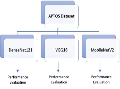
We first trained and validated MobileNetV2, DenseNet121 and VGG16 models using the APTOS dataset. We evaluated the models using accuracy, AUC and Kappa score. We found that MobleNetV2, even though is a lightweight network gives the best performance in terms of distinguishing between the classes (Figure 15, 16 and 17). Hence, we decided to conduct further experiments using MobileNetV2, since this is a multiclass classification problem.

We trained our MobileNetV2 network using 12 GB of RAM, 10 GB swap memory having i5 processor. We trained our MobileNetV2 model, applied the preprocessing and hyperparameter tuning settings mentioned earlier and achieved an accuracy of 91.68% on the test set mainly due to the good quality images that we fed into the network. The accuracy rapidly improved over the 20 epochs. (Figure 14)

We used a width multiplier of 1.4 and an input size of 224 x 224 x 3 for each input image. Table 4 shows the architecture of our network.