Chapter 5
Example 5.2-2. 6---
A tray tower is to be designed to absorb SO2 from an air stream by using pure water at 20oC. The entering gas contains 20 mol % SO2 and that leaving 2 mol % at a total pressure of 101.3 kPa. The inert gas flow rate is 150 kg air/h⋅m2, and the entering water flow rate is 6000 kg water/h⋅m2. Assuming an overall tray efficiency of 25%, how many theoretical trays and actual trays are needed? Assume that the tower operates at 20oC. Equilibrium data for SO2 – water system at 20oC and 101.3 kPa are given:
x 0 .0001403 .000280 .000422 .000564 .000842 .001403 .001965 .00279
y 0 .00158 .00421 .00763 .01120 .01855 .0342 .0513 .0775
x .00420 .00698 .01385 .0206 .0273
y .121 .212 .443 .682 .917
Solution --- The vapor and liquid molar flow rates are calculated first
L XA b, + V YA t, = L XA t, + V YA b, V = 150/29 = 5.18 kmol inert air/h⋅m2
L = 6000/18 = 333 kmol inert water/h⋅m2
We have yb = 0.20, yt = 0.02, and xt = 0. For the solute-free basis
A X = 1 A A x x − , YA = 1 A A y y − , A t X = , , 1 A t A t x x − = 0 1 0− = 0 , A t Y = , , 1 A t A t y y − = 0.020 1 0.020− = 0.0204 , A b Y = , , 1 A b A b y y − = 0.20 1 0.20− = 0.250 , A b
X can be determined from the component balance (A = SO2): L XA b, + V Y = A t, L XA t, + V YA b,
6
Geankoplis, C.J., Transport Processes and Separation Process Principles, 4th edition, Prentice Hall, 2003, p. 663
, A b X = XA t, + V L YA b, − V L YA t, , A b X = 0 + 5.18 333 ×0.250 − 5.18 333 ×0.0204 = 0.00357
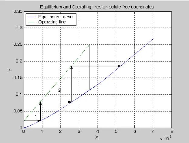
The operating line and the equilibrium curve can be plotted using the following Matlab codes: % Example 5.2-2 xe=[0 .0001403 .000280 .000422 .000564 .000842 .001403 .001965 .00279 .00420 .00698]; ye=[0 .00158 .00421 .00763 .01120 .01855 .0342 .0513 .0775 .121 .212]; Xe=xe./(1-xe);Ye=ye./(1-ye); X=[0 .00357];Y=[.0204 .25]; plot(Xe,Ye,X,Y,'--')
legend('Equilibrium curve','Operating line',2) xlabel('X');ylabel('Y')
Title('Equilibrium and Operating lines on solute free coordinates') grid on
Figure E-1 Theoretical number of trays.
The number of theoretical trays is determined by simply stepping off the number of trays as shown in Figure E-1. This gives 2.4 theoretical trays. The actual number of trays is 2.4/.25 = 10 trays.
Example 5.2-3. 6---
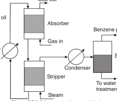
A waste airstream from a chemical process flows at the rate of 1.0 m3/s at 300 K and 1 atm, containing 7.4% by volume of benzene vapors. It is desired to recover 85% of the benzene in the gas by a three-step process. First, the gas is scrubbed using a non-volatile wash oil to absorb the benzene vapors. Then, the wash oil leaving the absorber is stripped of the benzene by contact with steam at 1 atm and 373 K. The mixture of benzene vapor and steam leaving the stripper will then be condensed. Because of the low solubility of benzene in water, two distinct liquid phases will form and the benzene layer will be recovered by decantation. The aqueous layer will be purified and returned to the process as boiler feedwater. The oil leaving the stripper will be cooled to 300 K and returned to the absorber. Figure E5.2-3 is a schematic diagram of the process.
Figure E5.2-3 Schematic diagram of the benzene-recovery process.
The wash oil entering the absorber will contain 0.0476 mole fraction of benzene; the pure oil has an average molecular weight of 198. An oil circulation rate of twice the minimum will be used. In the stripper, a steam rate of 1.5 times the minimum will be used.
Compute the circulation rate and the steam rate required for the operation. Wash oil-benzene solutions are ideal. The vapor pressure of oil-benzene at 300 K is 0.136 atm, and is 1.77 atm at 373 K.
Solution ---
For calculations in this example, subscript “a” will be used to indicate absorber and subscript “s” will be used to indicate stripper.
Molar rate of the gas entering the absorber is
Va,bot = 101, 300 1.0 8.314 300
×
× = 40.61 mol/s
6 Benitez, J. Principle and Modern Applications of Mass Transfer Operations, Wiley, 2009, p. 183
Gas out Gas in Absorber Stripper Steam Cooler Wash oil Condenser Separator Benzene product To water treatment plant
Molar rate of the carrier gas is given by a
V = Va,bot(1 −ya,bot) = 40.61×(1 − 0.074) = 37.61 mol/s
Converting the entering-gas mole fraction to mole ratio:
Ya,bot = a,bot a,bot 1 y y − = 0.074 1 0.074− = 0.0799
Converting the entering-liquid mole fraction to mole ratio:
Xa,top = a,top a,top 1 x y − = 0.0476 1 0.0476− = 0.0500
Since the absorber will recover 85% of the benzene in the entering gas, the concentration of the gas leaving will be
Ya,top = 0.15×0.0799 = 0.0120
The equilibrium data for the conditions prevailing in the absorber can be generated in the solute free basis from the following equation:
ya = 0.136xa [ From yaP = (Pbenzene)vapxa⇒ya(1 atm) = (0.136 atm) xa] a a 1 Y Y + = 0.136 a a 1 X X +
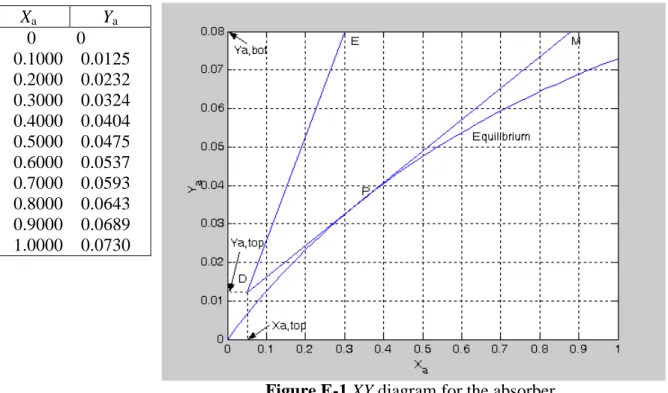
The following Matlab codes generate and plot the equilibrium data for the conditions in the absorber: X=0:0.02:1; a=0.136*X./(1+X); Y=a./(1-a); plot(X,Y) xlabel('X_a');ylabel('Y_a'); grid on line([0.05 0.3], [0.012 0.0799]) line([0.05 0.88], [0.012 0.08]) Gas out Gas in Absorber 85% recovery Liquid in Liquid out ya,top ya,bot xa,top = 0.0476 xa,bot = 0.074
The following table shows some of the equilibrium values generated from the Matlab codes. Xa Ya 0 0 0.1000 0.0125 0.2000 0.0232 0.3000 0.0324 0.4000 0.0404 0.5000 0.0475 0.6000 0.0537 0.7000 0.0593 0.8000 0.0643 0.9000 0.0689 1.0000 0.0730
Figure E-1 XY diagram for the absorber
Figure E-1 shows the equilibrium curve and the operating line for the absorber. Starting with any operating line above the equilibrium curve, such as DE, rotate it toward the equilibrium
curve using D as a pivot point until the operating line touches the equilibrium curve for the
first time. In this case the operating line DM touches the equilibrium curve at point P, a
location between the two end points of the operating line. The operating line DM corresponds
to the minimum solvent (oil) rate. From the diagram Xa,bot(max) = 0.88. Then a(min)
a
L
V =
a,bot a,top
a,bot(max) a,top
Y Y X X − − = 0.0799 0.012 0.88 0.050 − − = 0.0818
The minimum solvent rate is then: a
L (min) = 0.818×37.61 = 3.08 mol oil/s
For an actual oil flow rate which is twice the minimum La= 6.16 mol/s. The actual concentration of the liquid phase leaving the absorber is
Xa,bot = Xa,top + a a V L (Ya,bot− Ya,top) = 0.050 + 37.61 6.16 (0.0799 − 0.012) = 0.4646
We now consider the conditions in the stripper. Figure E5.2-3 shows that the wash oil cycles continuously from the absorber to the stripper, and through the cooler back to the absorber. Therefore Ls = La= 6.16 mol/s. The concentration of the liquid entering the stripper is the same as that of the liquid leaving the absorber (Xs,top = Xa,bot = 0.4646 mol of benzene/mol oil), and the concentration of the liquid leaving the stripper is the same as that of the liquid
entering the absorber (Xs,bot = Xa,top = 0.05 mol of benzene/mol oil). The gaseous phase entering the stripper is pure steam, therefore Ys,bot = 0.
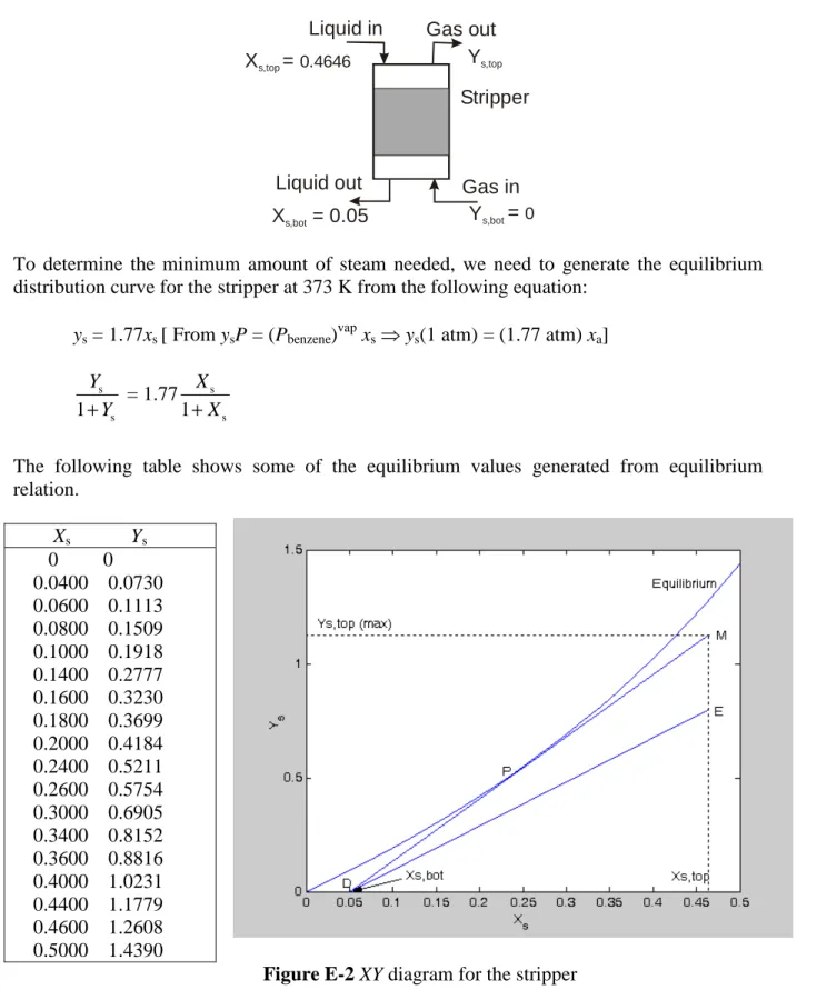
To determine the minimum amount of steam needed, we need to generate the equilibrium distribution curve for the stripper at 373 K from the following equation:
ys = 1.77xs [ From ysP = (Pbenzene)vap xs ⇒ ys(1 atm) = (1.77 atm) xa] s s 1 Y Y + = 1.771 s s X X +
The following table shows some of the equilibrium values generated from equilibrium relation. Xs Ys 0 0 0.0400 0.0730 0.0600 0.1113 0.0800 0.1509 0.1000 0.1918 0.1400 0.2777 0.1600 0.3230 0.1800 0.3699 0.2000 0.4184 0.2400 0.5211 0.2600 0.5754 0.3000 0.6905 0.3400 0.8152 0.3600 0.8816 0.4000 1.0231 0.4400 1.1779 0.4600 1.2608 0.5000 1.4390
Figure E-2 XY diagram for the stripper
Figure E-2 shows the equilibrium curve and the operating line for the stripper. Starting with any operating line below the equilibrium curve, such as DE, rotate it toward the equilibrium curve using D as a pivot point until the operating line touches the equilibrium curve for the
Gas out Gas in Stripper Liquid in Liquid out Ys,top Ys,bot Xs,top = 0.4646 Xs,bot = 0.05 = 0
first time. In this case the operating line DM touches the equilibrium curve at point P, a location between the two end points of the operating line. The operating line DM corresponds to the minimum steam rate. From the diagram Ys,top(max) = 1.13. Then
s (min) s L V = s,top s,bot s,top s,bot (max) Y Y X X − − = 1.13 0 0.4646 0.050 − − = 2.726
The minimum steam rate is then:
s
V (min) = 6.16
2.726= 2.26 mol steam/s
For an actual steam flow rate which is 1.5 times the minimum Vs= 1.5×2.26 mol/s = 3.39 mol/s. The actual concentration of the gas stream leaving the stripper is
Ys,top = Ys,bot + s s L V (Xs,top − Xs,bot) = 0 + 6.16 3.39(0.4646 − 0.05) = 0.753