Truly agent-oriented coupling of an activity-based demand generation with a multi-agent
traffic simulation
Marcel Rieser
Transport Systems Planning and Transport Telematics (VSP) TU-Berlin Salzufer 17-19, Sekr. SG 12 10587 Berlin Germany Phone: +49-30-314-25258 Fax: +49-30-314-26269 Email: [email protected] Ulrike Beuck
Transport Systems Planning and Transport Telematics (VSP) TU-Berlin
Phone: +49-30-314-29521 Fax: +49-30-314-26269 Email: [email protected] Jens Rümenapp
Gertz Gutsche Rümenapp Stadtentwicklung und Mobilität Büro Berlin Postfach 120361 10593 Berlin Germany Phone: +49-30-617-49430 Fax: +41-30-617-49433 Email: [email protected] Michael Balmer
Institute for Transport Planning and Systems (IVT) ETH Zurich 8093 Zürich Switzerland Phone: +41-1-633 27 80 Fax: +41-1-633 10 57 Email: [email protected] Kai Nagel
Transport Systems Planning and Transport Telematics (VSP) TU-Berlin
Germany
Phone: +49-30-314-23308 Fax: +49-30-314-26269 Email: [email protected]
1 ABSTRACT
The typical method to couple activity-based demand generation (ABDG) and dynamic traffic assignment (DTA) are time-dependent origin destination matrices. With that coupling method, the individual traveler's information gets lost. Delays at one trip do not affect later trips.
It is, however, possible to retain the full agent information from the ABDG by writing out all agents' “plans”, instead of the OD matrix. A plan is a sequence of activities, connected by trips. Since that information is typically already available inside the ABDG, this is fairly easy to achieve.
MATSim takes such plans as input. It iterates between the traffic flow simulation (sometimes called network loading) and the behavioral modules. The currently implemented behavioral modules are route finding, and time adjustment. Activity re-sequencing or activity dropping are conceptually clear but not yet implemented. Such a system will react to a time-dependent toll by possibly re-arranging the complete day; in consequence, it goes far beyond DTA (which just does route adaptation).
Our paper will report the status of our current Berlin implementation. The initial plans are taken from an ABDG, originally developed by Kutter; to our knowledge, this is the first time that traveler-based information (and not just OD matrices) is taken from an ABDG and used in a multi-agent simulation. The simulation results are compared against real world traffic counts from about 100 measurement stations.
2 INTRODUCTION
The arguably most advanced state-of-the-practice method for transport forecasting consists of the following three pieces:
• The process starts with an activity-based demand generation (ABDG). These do typically start from a synthetic population (1), and then add, to every potential traveler in the synthetic population, status (work/school/other), full activity patterns, activity locations, activity times, and possibly mode choice. Other sequences to add these elements are possible, and some or all of them may be generated jointly. Examples of practical applications of activity-based models can be found in San Francisco (2), Portland/Oregon (3), Florida (4), Toronto (5), or The Netherlands (6, 7). The typical outputs of an ABDG are time-dependent, e.g. hourly, origin-destination (OD) matrices.
• These hourly OD matrices are then taken and fed into a dynamic traffic assignment (DTA). A DTA assigns routes to time-dependent OD flows such that the routes in conjunction with their resulting traffic pattern fulfill some pre-defined criterion. For example, the routes may fulfill a Nash Equilibrium, meaning that at no time-of-day any OD flow can find a faster path. An often-used alternative criterion is a time-dependent Stochastic User Equilibrium (SUE), meaning that each OD flow is distributed across possible routes following a pre-specified distribution function at each point in time. – The typical way to solve the DTA problem is to use iterations between a router and a traffic simulation (also called network loading algorithm). Flows on routes that do not fulfill the pre-specified criterion are slowly adjusted into the right direction. The iterations stop when no more adjustments are necessary, i.e. when the iterations have reached a fixed point (8). Examples of DTA projects are Dynasmart (9), Dynamit (10), or a dynamic version of Visum (11).
• In order to close the feedback loop, spatial impedances – often in the form of inter-zonal travel times – are fed back from the DTA to the ABDG, and the feedback is iterated until a self-consistent solution is found. Although this feedback has been postulated a long time ago (12), it is, to our knowledge, usually implemented manually by the analyst, i.e. the analyst manually goes back and forth between ABDG and DTA until the solution is satisfying.
Unfortunately, this approach of coupling the ABDG and the DTA via OD matrices / link travel times can have several disadvantages:
• If a traveler is delayed in the morning, this may have temporal repercussions throughout the whole day. Such an effect is not picked up when travelers are converted into OD-streams.
• The traffic may have temporal patterns that go beyond hourly resolution (e.g. in reaction to a time-dependent toll). Hourly OD matrices cannot pick up such effects. In fact, even when feeding back 15-minute-averaged link travel times, the resulting travel time map can be highly distorted (13).
• When tolls are charged on certain links, the routing decision may depend on the travelers’ attributes, e.g. on income and/or on time pressure given by activities later during the day. Access to such information gets lost through the OD matrix.
• Some “higher level” decisions, such as mode choice or secondary activity location choice, may depend on relatively small details of the trip, such as walking distance to the public transit stop. Alternatively, mode choice may depend on one element of a complete tour, such as one location being not reachable by public transit. Such effects are straightforward to include when the DTA still knows about individual agents, but are impossible to pick up once travelers are aggregated into OD matrices.
In contrast, multi-agent simulations (MASim) of traffic process information about individual travelers at every level. Every modeled agent is assigned at least one “plan”, a series of activities and connecting
trips. The plan is made complete step by step by behavioral modules, inserting, say, activity patterns, activity locations, a mode choice decision, and finally precise routes and times. Since these processes occur in the travelers’ heads, we call this the “mental layer” of the MASim. Once all plans are complete, they are submitted to the traffic flow simulation, which attempts to execute them as faithfully as possible, given physical constraints caused by the system or by other travelers (e.g. congestion). Since the traffic flow simulation models physical processes, we call this the “physical layer” of the MASim. The distinction between the physical and the mental layer is taken from Multi-Agent Systems (14).
During the traffic flow simulation, the performance of every agent is recorded, e.g. by noting departure and arrival times at activity locations. From that performance information, the score (e.g. utility) of every plan is computed. During repeated iterations between the mental and the physical layer, every agent attempts to modify its plan so that it obtains a larger score. The choice dimensions along which the agents can learn are configurable. In this way, the simulation system can emulate dynamic traffic assignment (by only allowing the routes to adapt), or it can, say, simulate a system where agents’ residences, status, and primary activity locations are fixed, but everything else (secondary activity types and locations, mode, route, time scheduling) is adapted. Similarly, the scoring function is configurable, its only requirement being that it needs to allow to rank plans. In this way, not only standard utility functions (15) but also, say, prospect theory (16) can be included in a conceptually straightforward way.
An early attempt to use “true” agents that maintain their identity throughout the system (i.e. from the synthetic population generation through the activity-based demand generation and the router to the traffic flow simulation) was Transims (17). Its main shortcoming for a couple of years was that it was difficult to obtain and to use; now it is open source. Further differences between Transims and our approach are described below.
Another attempt to approach the problem is Metropolis (18). Metropolis uses one single OD matrix for the morning peak, and generates the temporal structure inside the DTA. That is, the time choice dimension is added to the route choice dimension inside the DTA.
Our own approach, MATSim (19), is based on Transims. It differs from Transims in several aspects, including: using just one hierarchical (XML) file format for the coupling between the behavioral modules (instead of several plain ASCII files); giving performance scores to full 24-hour plans based on the execution of those plans in the physical layer and using these scores for agent learning (instead of assuming that each new solution generated by a behavioral module is better than the solution before – an assumption that we found destructively invalid in certain situations (13)); and the use of a more lightweight, less data-hungry, and faster simulation of the physical layer – the queue simulation (20). In order to start the learning iterations of any MASim for traffic, initial conditions are needed. The most reasonable initial condition is a set of agents (synthetic population), where every agent has at least one plan where at least those elements that are not supposed to adapt during the learning iterations are defined.
It makes sense to look if existing methods can provide initial conditions for a MASim. The first thing to consider here are OD matrices, since they are so abundant in the community. Indeed, it is straightforward to extract individual trips from OD matrices, and to generate for each trip a “pseudo”-agent, whose complete plan consists of that single trip. This means, however, that trips that in reality belong together, since they are executed by a single traveler throughout the course of a day, are now completely decoupled. Therefore, no consistent adaptation between these trips is possible (e.g. time choice, location choice, tours mode choice); the only things that can be sensibly modified within the MASim are the routes.
Generating complete agents’ plans from OD matrices has also been tried, but is a complex and cumbersome process (21).
Fortunately, many implementations for ABDG (3, 4, 5, 6, 7, 22) internally use concepts that are much closer to agents, and aggregate the results to OD matrices only as their final step. It does, therefore, make sense to investigate if it is possible to output some other information from the ABDG that is easier to use by the MATSim.
In this paper we describe the steps taken to transform the individuals’ data from an existing ABDG into agents’ plans. The ABDG is based on the Kutter-Model (also known as Berliner Personenverkehrs-Modell) (23, 24, 25) for the region of Berlin, Germany. The plans are then used as input for our multi-agent traffic simulation MATSim (26). We will then compare the results of the simulation to real world data.
3 CREATING PLANS FROM ACTIVITY CHAINS
The Kutter-Model is a disaggregated, actvitiy- and behavior-oriented traffic demand generation model. It simulates the traffic demand using so-called “behaviorally homogeneous person groups (verhaltenshomogene Gruppen)” with the help of expectation values (23, 24, 25). This model is currently used to calculate daily OD-matrices for strategic planning, and was modified to output the internally used activity chains (27). The remainder of the paper describes how the ABDG data is used in our multi-agent simulation.
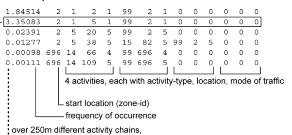
Each activity chain contains information about the start location (reference to a zone), up to four activities (limitation of the Kutter-Model), and the frequency of occurrence of the activity chain. The four activities are each described by their type, their location, and the transportation mode used to reach that location. Additionally, the activity chains are grouped, each group corresponding to one of 72 behaviorally homogenous groups with similar demographic attributes (see figure 1). The activity chains always describe trips that end at the same place as where they start (tours), while all activities between the first and the last activity take place somewhere else. The sum of all frequencies corresponds to the total number of tours accomplished by the people in the study area. There is no special provision for people who perform more than one tour per day – i.e. those tours are just listed separately; this leads to problems, as we will see later.
3.1 Time information
As one can see, much information needed for agents’ plans like activities and locations is available, with only the time information missing. Since the typical downstream applications of the Kutter model are 24-hour static assignments, this is not important, since all trips are just added up. MATSIM, however, deals with traffic as it unfolds over the day. Fortunately, MATSIM can generate its own timing information, which is generated and optimized over several iterations by a special module (28). Initially, all activities are assigned a random activity duration within a range, where the range depends on the type of the activity. These random durations are replaced, during the iterations, by more convenient durations by the mentioned module (see below).
3.2 From tour frequencies to agents
Based on the given description it seems possible to use all the information from the activity chains and transform them into agents’ plans. This would work without problems if the frequency of occurrence of each activity chain were an integer value. But the Kutter model does, in fact, output activity chain
frequencies which are often far below one: The model generates 7 million tours per day in our study area, but more than 250 million different activity chains are used to describe those tours.
This is not a problem in conventional assignment, where origin-destination-flows can be real numbers. It is also not a problem for certain types of DTA. It is, however, a problem for agent-based approaches such as MATSIM, where the smallest unit of flow is one agent. Thus, a way had to be found to deal with the fractional frequencies of activity chains.
FIGURE 1 The structure of activity chains generated by the Kutter-Model. There is one such file
for each “behaviorally homogeneous group”, i.e. 72 such files overall.
A simple approach would be to just round the frequencies to the next integer value and let that be the number of agents with that activity chain. Because of the special distribution of the frequencies (values range from less than 0.0001 up to the lower tens with an average value below 0.1), creating agents based on the rounded frequencies results in too few agents.
An alternative would be to accept each activity chain with a probability given by its frequency. (For frequencies larger than one, the probabilistic approach would only be used for the fractional part of the frequency.) This approach, however, suffers from strong fluctuations. For example, a start location that contains 10 activity chains with a frequency of 0.01 each may obtain 10 agents by such an approach. It was therefore decided to use the following approach: Tour frequencies are summed up one after the other. Every time the sum reaches 1.0 or any higher value, an agent with a plan based on the current activity chain is generated, and the sum is reduced by 1.0. If the activity chains were in a random sequence, then our method would corresponds to a weighted random draw without replacement, where the number of draws corresponds to the number of agents. Since, however, our files are sorted by starting location, multiple agents with the same starting location can only be generated if the frequencies for all tours with that starting location sum up to more than one. This stratification effect is desired, but we find the exact consequences difficult to assess.
Finally, over 7 million agents with each one plan assigned were generated, representing the 7 million tours undertaken by the people in the study area.
It is quite important to note that the number of agents created does not represent the number of inhabitants in the area, but the number of tours performed in one day by the inhabitants. This means we have more agents in the simulation than there are in the real world, but the agents have shorter day plans than their real world counterparts. This causes problems with the automatic activity timing feature of Matsim: If there is no temporal relationship between two tours of one person on the same day, then it is possible and likely that the times the two activities are performed will overlap. Because of the missing information that one activity can only take place after another, there is currently no need to perform activities late in the day. Instead, the agents try to accomplish the activities during regular work-hours, starting in the morning.
3.3 Mode choice
MATSim, our multi-agent traffic simulation, is currently only able to simulate individual car traffic. Therefore, only agents using the car for transportation were considered for the simulation. Since the Kutter model contains the mode, this was straightforward to implement. All tours that did not use exclusively the car were excluded; there are, however, relatively few (<1%) intermodal trips that use the car. Erroneously, all trips that use the car as a passenger were included as car trips. This overestimates the car trips by about 13%. This will be corrected in future versions.
3.4 From zones to links
Every trip starts and ends at a link in MATSim. However, most ABDG, including the Kutter-Model, generate demand on the level of traffic zones. Thus we had to assign links to activity locations, respectively to the location where trips start and end.
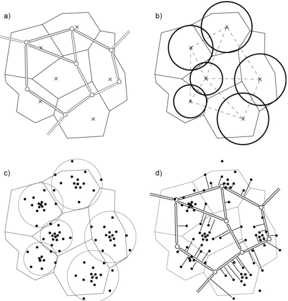
The following procedure was used to assign links to activity locations. In a first step, each activity is assigned a coordinate. In a second step, the nearest link to this coordinate is searched for and assigned to the activity. This 2-step procedure allows reusing the plans with different networks, as long as the coordinates are maintained. The coordinate is drawn randomly around the “centroid” of the traffic cell using polar coordinates. (In our data set, these points are not really “centroids” in the technical sense, but we use the term anyway.) By randomly choosing an angle and randomly choosing the distance, the density around the center of the circle is higher than it is on the border of the circle. This corresponds to the different population densities in the center of a village and the rural areas. The maximal distance a point can be located away from the centroid is 0.7 times the distance from the centroid to its nearest neighbor. The factor 0.7 has proved to lead to a good coverage of the circle areas while keeping overlaps low. Figure 2 gives a graphical overview how links are assigned to activity locations.
FIGURE 2 Assignment of links to activity locations. (a) Given a region consisting of zones, each zone having a “centroid”, and a network with nodes and links. (b) Circles are defined around zones’ centroids. (c) Activity locations are randomly chosen within the circle for each zone. (d) The activity locations are assigned to the nearest link.
4 SIMULATION AND SCORING
Once the agents’ plans are available, the simulation process can start. MATSim (19, 26) iterates between the traffic flow simulation (physical layer; sometimes called network loading) and the behavioral modules (mental layer). The traffic flow simulation moves the agents through the network according to their plans and generates events (e.g. vehicle entered or left a link, agent departs or arrives at an activity location) from which travel times, travel speeds, link densities, and other characteristics can be calculated. At the end of an iteration, each plan is evaluated regarding how successful the agent was performing the (planned) activities, resulting in a score for the plan (29). Scoring a plan is a precondition so that agents learn and react toward congestions or tolling. Different plans can be compared and an agent can pick the one with the highest value. A higher score implies that the agent makes better use of its day.
As scoring function, the traditional utility function based on the Vickrey bottleneck model is used (30), but modified to be consistent with complete day plans. Scoring is based on events information from the physical layer. Performing an activity is rewarded; travel times and late arrival are punished. The overall equation is:
!
!
!
+ + = i latei i travi i acti plan U U U U , , , (1)We assume the utility of performing an activity as increasing logarithmically:
! ! " # $ $ % & '' ( ) ** + , -= 0 ,( ) max 0, ln t x x Uacti . (2)
where x is the duration that the agent spends at the activity. We take
! "=#dur$t *, where ! "dur is uniformly
the same for all activities and only
!
t* varies between activity types. With this formulation,
!
t* can be interpreted as a “typical” duration, and
!
"dur as the marginal utility at that typical duration:
dur dur t x i act t t x U ! ! " " = = # # = * * , 1 * (3)
t0 can be seen as a minimum duration of an activity, but is better interpreted as a priority: All other things
being equal, activities with large t0 are less likely to be dropped than activities with small t0 (29).
The utilities of traveling and of being late are both seen as disutilities, which are linear in time:
x x
Utrav,i( )="trav! (4)
(where x is the time spent traveling) and
x x
Ulate,i( )="late! (5)
(where x is the time an agent arrives late at an activity).
!
"trav is set to -6 €/h, and
!
"late is set to -18 €/h. In principle, arriving early or leaving early could also be punished. There is, however, no immediate need to punish early arrival, since waiting times are already indirectly punished by foregoing the reward that could be accumulated by doing an activity instead (opportunity cost). In consequence, the effective (dis)utility of waiting is already -6 €/h. Similarly, that opportunity cost has to be added to the time spent traveling, arriving at an effective (dis)utility of traveling of -12 €/h. No opportunity cost needs to be added to late arrivals, because the late arrival time is already spent somewhere else. In consequence, the effective (dis)utility of arriving late remains at -18 €/h. These effective values are the standard values of the Vickrey model (30).
It would make sense to consider an additional punishment (negative reward) for leaving an activity early. This would describe, for example, the effect when there are, on a specific day, better things to do than to continue to work, but some kind of contract (e.g. shop opening hours) forces the agent to remain at work. A fixed percentage of agents will re-plan its day plan with one of the behavioral modules. The currently implemented behavioral modules are route finding and time adjustment. Using route finding, agents try to find better routes, but do not change their departure times or the duration of activities. To find better routes, they make use of the events to calculate actual link travel times and thus recognize jammed links. Using time adjustment, the departure times and activity durations are modified with the goal to optimize the individuals’ plans score (Balmer et al, in press). Additional behavioral modules are conceptually clear, but not yet implemented: Activity re-sequencing would change the order of activities (e.g. shopping
after work instead of before work), activity dropping would remove certain activities in an overloaded plan, or activity re-location would change an activity’s location.
When re-planning, an agent keeps its original plan and modifies a copy of it. Thus, an agent collects more and more variants of plans it can perform. Each agent can remember a configurable number of plans. If a behavioral module generates more than that, the plan with the worst score will be removed to store the new one.
Such a system with several different behavioral modules and adjusted scoring algorithms will react to a time-dependent toll by possibly re-arranging the complete day; in consequence, it goes far beyond DTA, which just does route adaptation.
The simulation is stopped when the agents’ average score does no longer significantly improve. 5 SCENARIO SETUP
5.1 Study area
The chosen study area of Berlin and its surroundings—namely the federal state of Brandenburg—covers an area of 150 x 250 km and has a population of about 6 million inhabitants. We focus on the urban area of Berlin; therefore this part of the region is represented with a much higher level of detail and accuracy than Brandenburg regarding network and demand.
5.2 Road network
The road network was originally developed by the planning department of the city of Berlin (Senatsverwaltung für Stadtentwicklung). It has been used as part of the city’s forecast model representing the supply side of the year 2015. Manual changes were necessary in order to exclude modifications of the road network planed until 2015.
Nodes are described by their coordinates, and links connecting these nodes form the network. The network links are described by their major attributes like length, free flow speed, number of lanes, and capacity. These network attributes are sufficient for our queue simulation. Unfortunately, the number of lanes is not needed for traditional assignment, and in consequence the quality of the data is often poor. In addition, capacity is in fact just a calibration factor in static assignment, and may be quite unrelated to the “hard” capacity needed by the queue simulation. Both issues will be discussed in a bit more detail below. The network has been used for mid term or long term transportation planning in Berlin with a scope of 24 hours. The demand is described by daily OD-matrices, which are based on defined traffic analysis zones (TAZ), and where the different matrices refer to different types of traffic (passenger, freight, …). Such demand is assigned to the network using static assignment according to defined capacity speed functions. As stated above, the official transport model has a scope of 24 hours; no further level of detail like time-dependent matrices is used. Thus, further modifications were necessary in order to use the input data for our multi-agent simulation.
The most crucial attribute of a network link is its (flow) capacity, which is interpreted differently by the aggregated model used by the planning department of Berlin and the multi-agent simulation used by us. In our simulation, capacity is understood as maximum outflow of a link in a given time period, while the model of the planning department does not treat capacity values as hard constraints The traffic assignment method uses suitable functions to relate capacity and flow with the resulting cost in terms of
travel times. Thus, we had to adapt the theoretical capacity values that were the basis for a 24 hours static assignment. That was achieved by considering some of the larger streets and their maximum flow rates in reality, and comparing those to the numbers in the data file. From this, a capacity period of 12 hours was derived, i.e. the capacity numbers from the assignment file were divided by 12 in order to obtain the hourly capacities for our model. In addition, capacities were multiplied by 1.3 to compensate for the overestimation of the demand as explained earlier. This will be corrected in future versions.
Additionally, the storage of a link is constrained. The storage of a link can be calculated as length times the number of lanes divided by the space a vehicle occupies in a jam (7.5 m). Unfortunately, the number-of-lanes attribute is set to be one on all links of the original network. Since the number of lanes is not necessary for static assignment, such a network error is tolerated in the aggregated model. In our simulation, we currently set the number of lanes to two in order to calculate maximum storage, but a better solution has to be found in the near future.
The final road network representation consists of more than 10,000 nodes and almost 30,000 links connecting those nodes. As stated above, the demand data that is available for Berlin does only consist of daily OD-matrices. This kind of demand data is only sufficient for strategic long term transportation planning. Multi-agent based simulations require the demand to be given on the individual level as day-plans containing the activities with the scheduling and location information and the trips between them. 5.3 Scaling
In order to speed up the Berlin scenario, the demand and the network capacities where scaled down to 10 % of the actual values.
6 RESULTS
The average score of all agents’ plans gives usually a good overview of the iterations’ progress. In the first iterations, the average score is low as the system is far away from being relaxed. With ongoing iterations, the agents learn how to avoid traffic jams by choosing different routes or starting their trips at different times of day. Figure 3 shows the average score of the first 80 iterations. The improvement of the average score is enormous in the beginning, but slows down later as more and more agents find better times and routes for their plans. After iteration 50, the behavioral module for time adjustment is deactivated, while the behavioral module for route finding is deactivated after iteration 60. As can be seen in figure 3, the score improves slightly both times when a behavioral module is switched off. This can be explained by the reduction of the amount of re-planning agents. In the first few iterations, a high amount of re-planning agents is desirable to quickly move to a better solution than the initial one. But after some iterations, a too large number of planning agents can lead to instabilities: When every re-planning agent searches for the fastest or shortest route from one activity to another, new traffic jams can be initiated as many of the agents will select the same link for similar route-sections. By switching off behavioral modules and thus reducing the amount of re-planning agents, the probability of such traffic jams is reduced, leading to shorter travel times for the agents and thus to a higher average score. After iteration 60, each agent selects in each iteration one of its remembered plans for simulation. Assuming a relaxed state was reached before iteration 60, this usually leads to a simulation of traffic in a relaxed network with small fluctuations as can also be observed in the real world.
FIGURE 3 The agents’ average score of the first 80 iterations.
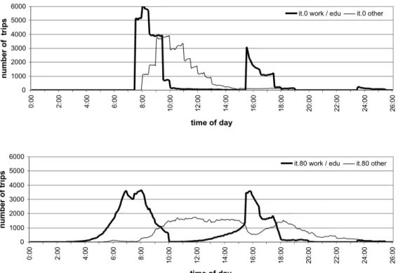
Adjusting trip departure times and activity durations are the most efficient ways to get a relaxed system. Initially, all agents are assigned random start time for the first activity and random activity durations, each within a certain range of time. The range depends on the type of the activity. Each time an agent re-plans, the agent tries to optimize its possible score by re-allocating activity-durations (28). This leads to a differentiated distribution of trip departure times. Figure 4 shows the number of trip departures over the course of a day, in the upper part for the initially assigned times in iteration 0 and in the lower part for iteration 80, where the times were optimized during the iterations to nearly reach a relaxed system. The numbers of trip departures are furthermore differentiated between trips of plans having work or education as primary activity, and plans having other primary activities like shopping or leisure. It can be seen that the agents try to avoid traffic jams in the morning by leaving home earlier than initially assigned. Additionally, agents that do not have to work or go to school and thus are more flexible, try to avoid the evening rush hour by performing trips before or after the peak hour.
FIGURE 4 The number of trip departures over the course of a day in iteration 0 (top) and iteration 80 (bottom), differentiated by the type of the primary activity of the corresponding plan.
We have data from about 100 measurement stations in Berlin where the traffic passing by was measured. The counts are available in hourly slices, but not all measurement stations have values for every hour of a day. Only a few stations offer counts for the whole day, while many stations only have counts for the morning rush hour.
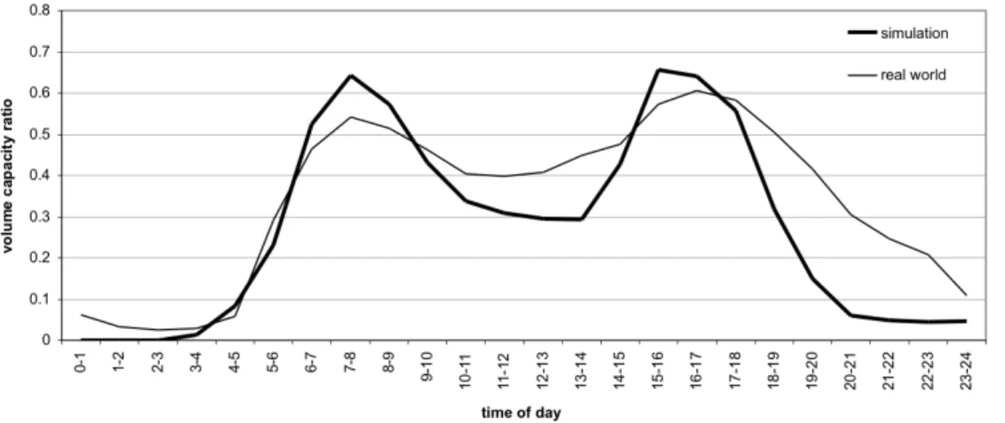
We can compare these counts for each measurement station to the number of vehicles that travel across the corresponding links in our simulation during the time period of interest. Alternatively, we can calculate an average volume capacity ratio of all measurement stations based on the links’ capacities. For this, we sum up the capacities of all links we have counts for in a specified hour. Next, we sum up the counts for those links. With these two sums, an average volume capacity ratio can be calculated for the specified hour. The same can be done for the number of vehicles on those links in the simulation. Figure 5 shows the two volume capacity ratios in comparison over the course of a day. Note how our system can trace the evolution of that number as a function of the time-of-day.
It can be seen that the average volume capacity ratio is generally lower in the simulation than it is in the real world, except during the morning and evening hours. The missing traffic between morning and evening can be explained with the lack of commercial traffic in the Kutter-Model. The overestimation of traffic during the peak hours, together with the underestimation of traffic in the evening, may be explained with the input-data only containing tours but not complete day plans. As was explained at the end of Sec. 3.2, the Kutter model generates tours that belong to the same person completely separately. In consequence, all these tours will have a tendency to start in the morning.
FIGURE 5 A comparison of average volume capacity ratios over the course of a day.
For each measurement station, a relative error can be calculated for every hour data is available. The relative error is defined as the absolute difference between real world and simulated counts, divided by the real world counts. An average of the relative error over all measurement stations can be plotted. As can be seen in figure 6 the average relative error changes over the course of the day. It is relatively high during the night and improves during the course of the day. The large error during the night can be explained by the fact that during the night, the divisor (real world traffic counts) is relatively small. These numbers need to be taken as an indication of where we are, not where we want to be. In fact, in previous studies (in Zurich) we have achieved relative errors according to the same benchmark that were around 0.3 instead of around 0.6. This is also our goal for Berlin.
7 DISCUSSION AND FUTURE WORK
Our work has shown that it is possible to couple ABDG with multi-agent traffic simulations. Nevertheless, the results are not yet satisfying. While it is possible to re-use internal data from ABDG, the data has, at least in our case, some severe shortcomings. If data should be used from ABDG for multi-agent simulations, these shortcomings must first be recognized and then overcome. Either this can be done by modifying the ABDG itself, or the internal data needs to be more thoroughly post-processed to make it suitable for multi-agent simulations.
A major shortcoming is that each agent in the simulation corresponds to a route, but not to a “real” person. This can be seen in the number of agents (7m agents compared to 6m inhabitants) as well as in the fact that every agent is only at home at the start and the end of a plan, but never in-between two activities (e.g. having lunch at home). This leads to missing temporal relationships between trips and too little traffic in the evening, as shown in chapter “Results”. Combining two or more activity chains into one agent would reduce the number of agents, while at the same time it would increase the average complexity of a plan. The combination of several activity chains into one plan must be done carefully and needs some research first, as not every combination of activity chains has the same probability. But the fewer but longer plans might help to relax the pressure in the morning hours and might lead to an increased amount of traffic later in the day.
If ABDG were modified to include complete day plans, an important step would be made towards agent-based demand generation. This would not only be useful for our agent-agent-based simulation, but in fact for any dynamic traffic assignment that takes time-dependent information as input.
Some segments of the traffic, such as long distance traffic, tourists, business travelers, and commercial traffic, are missing. In principle, those segments could be handled by agent-based models similar to the one described in this paper. Alternatively, and arguably more pragmatically, one could handle those trips by adding single trips based on conventional OD matrices for those travel segments only. This is indeed what we intend to do for Berlin.
Our results have to be interpreted with regard to Berlin’s special history. The partition of the city into two parts by the wall and the reunification led to a city having more than one center. Additionally, the behavior of some parts of the population (mainly those of older generations) still differs based on their origin and historical background. This requires special modifications of the behavioral modules and the algorithm used for scoring. The amount of modifications must yet be figured out.
Additionally, the data for the Berlin scenario must be further improved. Some attributes of the network provided by the planning department of the city of Berlin cannot be reconstructed or fully understood, while other attributes (like the number of lanes per link) are completely missing. We currently use heuristics to overcome these shortcomings, but having the correct values from the source of the data would clearly help to improve the results of the simulation.
8 ACKNOWLEDGMENTS
Many thanks to Dr. Imke Steinmeyer—without her this project would not have been possible. She organized the exchange of data from the Kutter-Model, building the base for this project. Additional thanks go the planning department of Berlin (Senatsverwaltung für Stadtentwicklung). They provided us with the network used in this study and gave permission to use the data from the Kutter-Model.
We would like to thank Konrad Meister for his work on planomat. Without his comprehensive activity scheduler, our simulations would take a lot longer until they reached a relaxed state.
Furthermore, we would like to thank the Volvo Research and Educational Foundations for granting funding for the research project “Environmentally-oriented Road Pricing for Livable Cites”.
9 REFERENCES
1. Beckman, R. J., K. A. Baggerly, and M. D. McKay. Creating synthetic base-line populations. Transportion Research Part A – Policy and Practice, 30(6):415–429, 1996.
2. Jonnalagadda, J., N. Freedman, W.A. Davidson, and J.D. Hunt. Development of microsimulation activity-based model for San Francisco: destination and mode choice models. Transportation Research Record, 1777:25–35, 2001.
3. Bowman, J. L., M. Bradley, Y. Shiftan, T.K. Lawton, and M. Ben-Akiva. Demonstration of an activity-based model for Portland. In World Transport Research: Selected Proceedings of the 8th World Conference on Transport Research 1998, volume 3, pages 171–184. Elsevier, Oxford, 1999. 4. Pendyala, R. M. and R. Kitamura. FAMOS: The Florida Activity Mobility Simulator. In H.J.P.
Timmermans, editor, Progress in activity-based analysis. Elsevier, Oxford, UK, In press.
5. Miller E. J. and M.J. Roorda. A prototype model of household activity/travel scheduling. Transportation Research Record, 1831:114–121, 2003.
6. Arentze, T. A. and H.J.P. Timmermans. Albatross: A Learning-Based Transportation Oriented Simulation System. EIRASS, Eindhoven, NL, 2000.
7. Arentze, T. A. and H.J.P. Timmermans. ALBATROSS – Version 2.0 – A learning based transportation oriented simulation system. EIRASS (European Institute of Retailing and Services Studies), TU Eindhoven, NL, 2005.
8. Watling, D. Asymmetric problems and stochastic process models of traffic assignment. Transportation Research B, 30(5):339–357, 1996.
9. DYNASMART www page, accessed 7/2006. URL www.dynasmart.com. 10.DYNAMIT www page, accessed 7/2006. URL mit.edu/its.
11.Friedrich, M., I. Hofsäß, K. Nökel, and P. Vortisch. A dynamic traffic assignment method for planning and telematic applications. In Proceedings of Seminar K, volume P445 of European Transport Conference, pages 29–40, Cambridge, GB, 2000. PTRC. ISBN 0-86050-341-0.
12.Loudon, W.R., J. Parameswaran, and B. Gardner. Incorporating feedback in travel forecasting. Transportation Research Record, 1607:185–195, 1997.
13.Raney, B. and K. Nagel. Iterative route planning for large-scale modular transportation simulations. Future Generation Computer Systems, 20(7): 1101–1118, 2004. ISSN 0167-739X.
14.Ferber, J. Multi-agent systems. An Introduction to distributed artificial intelligence. Addison-Wesley, 1999.
15.Jara-Diaz, S. et al. Modelling activity duration and travel choice from a common microeconomic framework. In Proceedings of the meeting of the International Association for Travel Behavior Research (IATBR), Lucerne, Switzerland, 2003. See www.ivt.baum.ethz.ch.
16.Avineri, E. and J.N. Prashker. Sensitivity to uncertainty: Need for paradigm shift. Paper 03-3744, Transportation Research Board Annual Meeting, Washington, D.C., 2003.
17.TRANSIMS www page, accessed 7/2006. URL www.transims.net
18.de Palma, A. and F. Marchal. Real case applications of the fully dynamic METROPOLIS tool-box: an advocacy for large-scale mesoscopic transportation systems. Networks and Spatial Economics, 2(4):347–369, 2002.
19.MATSIM www page, accessed 7/2006. URL www.matsim.org
20.Cetin, N., A. Burri, and K. Nagel. A large-scale agent-based traffic microsimulation based on queue model. In Proceedings of Swiss Transport Research Conference (STRC), Monte Verita, CH, 2003. URL www.strc.ch. Earlier version, with inferior performance values: Transportation Research Board Annual Meeting 2003 paper number 03-4272.
21.Balmer, M., M. Rieser, A. Vogel, K.W. Axhausen, and K. Nagel (2005): Generating day plans using hourly origin-destination matrices. In T. Bieger, C. Laesser, and R. Maggi, editors, Jahrbuch 2004/05 Schweizerische Verkehrswirtschaft. St. Gallen. pages 5–36.
22.Bhat, C. R., J.Y. Guo, S. Srinivasan, and A. Sivakumar. A comprehensive econometric microsimulator for daily activity-travel patterns (cemdap). Transportation Research Record, forthcoming. Also see www.ce.utexas.edu/prof/bhat/FULL_REPORTS.htm.
23.Kutter, E. (1984): Integrierte Berechnung städtischen Personenverkehrs – Dokumentation der Entwicklung eines Verkehrsberechnungsmodells für die Verkehrsentwicklungsplanung Berlin (West). Berlin.
24.Kutter, E., H-J. Mikota (1990): Weiterentwicklung des Personenverkehrsmodells Berlin auf der Basis der Verkehrsentstehungsmatrix 1986 (BVG). Untersuchung im Auftrag des Senators für Arbeit, Verkehr und Betriebe. Berlin.
25.Kutter, E., H-J. Mikota, J. Rümenapp, and I. Steinmeyer: Untersuchung auf der Basis der Haushaltsbefragung 1998 (Berlin und Umland) zur Aktualisierung des Modells "Pers Verk Berlin / RPlan", sowie speziell der Entwicklung der Verhaltensparameter ’86 - ‘98 im Westteil Berlins, der Validierung bisheriger Hypothesen zum Verhalten im Ostteil, der Bestimmung von Verhaltensparametern für das Umland. Entwurf des Schlussberichts im Auftrag der Senatsverwaltung für Stadtentwicklung Berlin. Berlin / Hamburg.
26.Raney, B. and K. Nagel (2005): An improved framework for large-scale multi-agent simulations of travel behavior. Paper 05-1846, Transportation Research Board Annual Meeting, Washington, D.C., 2003.
27.Rümenapp, J and I. Steinmeyer (2006): Activity-based demand generation: Anwendung des Berliner Personenverkehrsmodells zur Erzeugung von Aktivitätenketten als Input für Multi-Agenten-Simulationen. Arbeitsberichte Verkehrssystemplanung und Verkehrstelematik Nr. 06-09. TU Berlin. 28.Meister, K., M. Balmer, K.W. Axhausen, K. Nagel (2006): planomat: A comprehensive scheduler for
a large-scale multi-agent transportation simulation. In Proceedings of Swiss Transport Research Conference (STRC), Monte Verita, CH, 2006. URL www.strc.ch.
29. Charypar, D. and K. Nagel (2005): Generating complete all-day activity plans with genetic algorithms. Transportation, 32(4):369-397.
30. Arnott, R., A. De Palma, and R. Lindsey (1993). A structural model of peak-period congestion: A traffic bottleneck with elastic demand. The American Economic Review, 83(1):161.