Mathematical Model of Data Backup and Recovery
Karel Burda
The Faculty of Electrical Engineering and Communication Brno University of Technology, Brno, Czech Republic Summary
The data backup and data recovery are well established disciplines within the computer science already. Despite this fact, however, there is currently no sufficiently general mathematical
model for quantification of backup strategies. In this paper, such
mathematical model is derived. The model introduced is based on the assumption that the total size of the data is constant. Using this model, we can quantitatively evaluate the properties of different types of backup strategies. For the full, differential and incremental backup strategies, formulae are derived for the calculation of the average total backup size and the average data recovery size in dependence on the probability of the change of data units. The quantitative relations obtained are discussed. Key words:
Data backup, data recovery, mathematical model.
1. Introduction
Data are one of the most valuable assets of persons and organizations. However, we can lose these data due to technical failures, human errors, etc. This is the reason why data are copied into backup data repositories (so-called data backup) in order to have the possibility of reconstructing these data when the data are lost in the main data repository (so-called data recovery).
With regard to mathematical models of backup processes, A. Frisch states that “studies performing numerical and quantitative modeling backup processes are surprisingly rare” (see [1], p. 234). The models published so far allow only computations of full and incremental backups (e.g. [2], p. 4) and the quantification of the Amanda backup scheme ([3], p. 745-750 or [1], p. 225-229). Z. Kurmas and L. Chervenak have published a comparison of some backup strategies [4], however, their evaluation of backup strategies is based on simulations and therefore no analytic results are presented in this paper. Other research papers are oriented on backup frequency and timing (e.g. [5] or [6]) and also do not provide any suitable results for the evaluation of general backup strategies. Therefore, we can state that there is currently no sufficiently general mathematical model for quantification of data backup and recovery, despite the great importance of both of these procedures. This paper introduces a mathematical model of data backup which allows a quantitative comparison of different backup methods.
In the next section, the basic terms are formulated and the process of data backup and recovery is formalized. The third section is dedicated to the schemes of data recovery and the fourth section deals with the atomic backup (backups based on snapshots of data units). In the fifth section, a mathematical model for the quantification of backups is derived and in the sixth section, this model is applied to different data backup methods and the results obtained are discussed.
2. Data backup formalization
The terminology of the data backup is not unified and many authors “are using the basic terms in different and often conflicting ways” [7]. Therefore, we specify and formalize basic terms at first.
Data D are a structure of symbols, which represents some information. In the data repository, these data are arranged into certain elementary (i.e. further indivisible) sequences of symbols (e.g. sectors of the hard disk). We refer to an elementary sequence d of symbols as a data unit and denote the x-th data unit as dx. In the course of time,
the data unit dx can correspond to different sequences of
symbols, which we call versions of the data unit dx. The
data unit dx, which does not represent any information, is
the so-called empty data unit. We will formally denote such a data unit as dx = −. The model is based on the
assumption that the total size of the data D is constant and that the size of the metadata (overhead of data units) is negligible.
We have already stated that the symbol sequence of the data unit dx varies with time t. From the backup
viewpoint, the important events are changing the data units and taking the backups. To simplify description, we assume that the events mentioned can not come simultaneously and changing the data units and taking the backups are instantaneous, i.e. the duration of these events is equal to zero. When the data unit dx has been changed at
the time ti, we denote this version of the data unit as dx(ti). This version is valid in the time interval 〈ti, tj), where tj is
the instant of the next change of the data unit dx. The
quantity dx(ti) can also represent a version of the data unit
which is valid at the time ti. In our model, we assume that
We will denote the data at the instant ti as D(ti) and
assume that these data consist of n data units d1(ti) to dn(ti). Then, we can formally represent the data as an array
of n data units:
[
( ), ( ), , ( )] [
( )]
. )(ti d1 ti d2 ti dn ti dx ti xn1
D = = = (1)
The basis of any arbitrary type of backup is the full backup. The full backup F(ti) is a record of all data units which were valid at the time ti, i.e.:
F(ti) = D(ti). (2)
Full backups are large, because they also contain data units which have remained unchanged since the previous backup. Therefore, these backups are combined with partial backups, which contain only data which have been changed compared to some previous backup.
Let D(tj) be the data at the instant tj and let D(ti) be
the data at the instant ti. Denote by bx(ti, tj) the change of
the data unit dx at the instant tj in contrast to the instant ti.
It holds for this change:
= − = otherwise. ), ( , ) ( ) ( when , 0 , deleted been has when , ) , ( j x j x i x x j i x t d t d t d d t t b (3)
The first line expresses the situation when the data unit dx
has been deleted, the second line represents the situation when there has been no change in the data unit dx and the
third line corresponds to the situation when the data unit dx
has been either created or modified.
Then, the partial backup P(ti, tj) is a total of changes
of all data units within the interval (ti, tj〉:
[
( , )]
. ) , ( 1 n x j i x j i t b t t t P = = (4)It generally holds that bx(ti, tj) ≠ bx(tj, ti) and therefore P(ti, tj) ≠ P(tj, ti). For example, when D(t1) = [d1(t1),
d2(t1), d3(t1)] and D(t2) = [d1(t1), d2(t2), −], then P(t1, t2) = [0, d2(t2), −] but P(t2, t1) = [0, d2(t1), d3(t1)].
When we know the data D(ti) and the partial backup P(ti, tj), then we can recover D(tj), i.e. data at the instant tj.
Let us define an operation within which the data D(tj) are
recovered from the data D(ti) and the partial backup P(ti, tj). We refer to this operation as a data revision. Formally, we define the data revision in the following way:
) ( ) , ( ) (ti P ti tj Dtj D = , (5)
where the revision of each data unit is given by the formula: = − = − = = = otherwise. ), , ( , 0 ) , ( when ), ( , ) , ( when , ) , ( ) ( ) ( j i x j i x i x j i x j i x i x j x t t b t t b t d t t b t t b t d t d (6)
In the case of the first line, the backup contains the information that the data unit dx has been deleted in the
course of the time interval (ti, tj〉. For this data unit, the
result of data revision is an empty unit. In the case of the second line, the backup contains the information that there has been no change in the data unit dx in the given interval.
For this data unit, the result of data revision is the version of the data unit at the instant ti. The third line corresponds
to the situation when the backup contains the changed version of the data unit dx. In this case, the result of data
revision is the changed version of the data unit.
When it holds for the data revision in (5) that ti < tj,
then we will speak about forward data recovery. In this case, we obtain by data revision a newer version, D(tj),
from the older version, D(ti). When it holds that ti > tj,
then we will speak about backward data recovery. In this case, we obtain by data revision the older version, D(tj),
from the newer version, D(ti). For our examples of
backups, it holds that:
[
] [
]
[
−] [
= −]
= = − = = ), ( ), ( ) ( ), ( ) ( , 0 ) ( ), ( , 0 ) ( ), ( ), ( ) , ( ) ( ) ( 2 2 1 1 1 3 2 2 1 2 1 1 2 2 1 3 1 2 1 1 2 1 1 2 t d t d t d t d t d t d t d t d t d t d t t P t D t D and[
] [
]
[
( ) 0, ( ) ( ), ( )] [
( ), ( ), ( )]
. ) ( ), ( , 0 ), ( ), ( ) , ( ) ( ) ( 1 3 1 2 1 1 1 3 1 2 2 2 1 1 1 3 1 2 2 2 1 1 1 2 2 1 t d t d t d t d t d t d t d t d t d t d t d t t P t D t D = − = = − = = When we do not need to distinguish between the full backup F(ti) and the partial backup P(tj, ti), then we will
generally denote these backups as B(ti).
We will classify partial backups into interval and atomic backups. An interval backup I(ti, tj) is a partial
backup P(ti, tj) which contains the latest version of the
data units that have been changed in the interval (ti, tj〉.
This means that if any data unit is changed several times in the interval (ti, tj〉, then the given interval backup will
contain only the version of the data unit which was valid at the instant tj. From this, it follows that we can recover the
state of data only for the instants of taking backups. This type of backup is historically the oldest and these backups have a smaller size.
The atomic backup is a modern method which has been made possible by the so-called snapshot technique (e.g. [8]). With this technique, when a new version of a data unit is written, the older version of the given data unit (the so-called snapshot) is retained in the repository. In the case of atomic backup, all snapshots are backed up and therefore we can recover the data into the state at an arbitrary instant. A drawback of this type of backup is the large size of the aggregate of all snapshots. Before we explain the atomic backups in more detail, we will first discuss the data recovery schemes.
3. Data recovery schemes
The scheme of data recovery defines the procedure of data reconstruction from the backups acquired. In this paper, we will express data recovery schemes by a graph. The nodes i and j of such a graph represent the backups
B(ti) and B(tj) and the oriented edge (i, j) expresses that we must first recover the data from the backup B(ti) and
subsequently revise these data by using the data from the backup B(tj). We will call this relation between backups as a backup succession. In this case, we will call the backup
B(ti) a reference backup and the backup B(tj) a subsequent
backup.
An example of the recovery scheme for five consecutive backups B(t1) to B(t5) is given in Fig. 1. The backup B(t1), i.e. node 1, is a full backup which contains all data at the instant t1. Simultaneously, this backup is the reference backup for the partial backups B(t2) and B(t4). These backups are reference backups for the partial backups B(t3) and B(t5). The interval backups B(t2), B(t3) and B(t5) contain changes of data units compared to the nearest previous backup. The interval backup B(t4) contains the latest version of the data units which were changed within the interval (t1, t4〉.
3 5
t1 t2 t3 t4 t5
t
1
2 4
Fig. 1: An example of a recovery scheme.
From Fig. 1, it is apparent that if we want to recover data at the instant t3, we must first write the full backup
B(t1) into the main repository, then we must revise these data by the backup B(t2), and finally, we must still revise the data obtained by using the backup B(t3).
Now, we can explain the recovery schemes more precisely. In this paper, we focus on the milestone, differential and incremental recovery schemes because these schemes are the most widely used. The above recovery schemes are associated with the full, differential and incremental backup strategies [9]. For our example of five backups, the aforesaid schemes are illustrated in Fig. 2 to Fig. 4. Fig. 2 illustrates the milestone recovery scheme. This scheme consists of full backups (the so-called milestones) only, i.e. B(ti) = F(ti). A drawback of this
recovery scheme is the large size of backups (a large capacity of backup repositories is required), but the data
recovery is very simple. The data D(ti) are simple to
recover by writing the full backup F(ti) into the main
repository, i.e.:
D(ti) = F(ti). (7)
1 2 3 4 5
t1 t2 t3 t4 t5
t
Fig. 2: An example of the milestone recovery scheme.
Other schemes are based on a combination of the full backup and partials backups. We will refer to these schemes as reference recovery schemes. The differential and incremental recovery schemes are the most frequently used. The differential recovery scheme is illustrated in Fig. 3. In this type of recovery scheme, the first backup B(t1) is the full backup and all the other backups are interval backups. The reference backup for each interval backup is the first backup. Formally, we can express this scheme as
B(t1) = F(t1) and B(ti) = I(t1, ti) where i = 2 to 5. The advantage over the previous scheme is the smaller size of the aggregate of backups but the recovery of D(ti) for i > 1
is more complicated. In this case, we first write the full backup F(t1) into the main repository at first and then we revise these data by the backup I(t1, ti). Formally, we can
express the data recovery according to the differential recovery scheme as:
= = otherwise. ), , ( ) ( , 1 for ), ( ) ( 1 1 1 i i t t I t F i t F t D (8) 2 3 4 5 t1 t2 t3 t4 t5 t 1
Fig.3: An example of the differential recovery scheme.
Fig. 4 illustrates the incremental recovery scheme. In this type of recovery scheme, the first backup B(t1) is again the full backup and all the other backups are interval backups. However, the reference backup for each interval backup is the nearest previous backup. Formally, we can express this scheme as B(t1) = F(t1) and B(ti) = I(ti− 1, ti)
where i = 2 to 5. The advantage over the two previous schemes is the smaller size of the aggregate of backups; however, the recovery of D(ti) for i > 1 is the most
complicated on the average. This is because data from the backup B(t1) must be sequentially revised by all backups
B(t2) to B(ti). Formally, we can express the data recovery
according to the incremental recovery scheme as:
= = −, ),otherwise. ( ... ) , ( ) ( , 1 for ), ( ) ( 1 2 1 1 1 i i i t t I t t I t F i t F t D (9) 1 2 3 4 5 t1 t2 t3 t4 t5 t
Fig. 4: An example of the incremental recovery scheme.
All the reference schemes described are forward data recovery schemes, i.e. we can recover the data D(tj) from
the initial full backup F(ti), where tj > ti. By analogy, there
are also backward data recovery schemes. In these cases, the reference full backup contains the newest data and the partial backups contain older versions of data units. If need be, we can return to a certain former state of the data. The representatives of backup systems with backward data recovery are some backup systems with data mirroring. Data mirroring (e.g. [10]) is based on that each change of any data unit in the main repository is practically instantly executed in the backup repository too. Therefore, the data in both repositories are identical and the backup repository can be used in the case of the failure of the main repository as a full-blown replacement of the impaired repository. When we back up older versions of data units, then from the valid data D(ti), we can restore data at the instant tj,
where tj < ti.
4. Atomic backup
Now, we can return to the description of the atomic backup. In the case of atomic backup, when a new version of the data unit is written, the older version of this data unit (the so-called snapshot) is retained in the repository. A backup program looks up and backs up snapshots which have not been backed up yet. By using the time data, which are kept about each snapshot, we can arrange the versions of all data units according to their validity in the time. This sequence allows us to recover data at an arbitrary instant. From the backup viewpoint, we can consider each snapshot as an individual backup. Then we can consider the sequence of snapshots in time as a sequence of individual backups, which are organized in the incremental recovery scheme. Each atomic backup always contains a single
version of a single data unit only. When the data unit dy is
changed at the instant ti, then we can formally express the
corresponding atomic backup A(tj, ti) as:
[
( , )]
, ) , ( 1 n x i j x i j t b t t t A = = (10) where = = otherwise. , 0 , for ), ( ) , (t t d t x y bx j i y i (11)Of course, the operation of data revision also holds for atomic backups.
We will illustrate the atomic backup on a scenario according to Table 1 and Fig. 5.
Tab. 1: A scenario for the illustration of the atomic backup.
ti d1(ti) d2(ti) d3(ti) Backups B t1 d1(t1) d2(t1) d3(t1) B(t1) = F(t1) = [d1(t1), d2(t1), d3(t1)] t2 d1(t1) d2(t2) d3(t1) B(t2) = A(t1, t2) = [0, d2(t2), 0] t3 d1(t1) d2(t2) d3(t3) B(t3) = A(t2, t3) = [0, 0, d3(t3)] t4 d1(t1) d2(t4) d3(t3) B(t4) = A(t3, t4) = [0, d2(t4), 0] t5 d1(t1) d2(t4) d3(t3) − 1 2 3 4 t1 t2 t3 t4 t5 t [d1(t1), d2(t1), d3(t1)] [0, d2(t2), 0] [0, 0, d3(t3)] [0, d2(t4), 0]
Fig. 5: An example of the atomic backup.
In this scenario, the data consist of three data units dx,
where x ∈ {1, 2, 3}. At the instant t1, three data units
d1(t1), d2(t1) and d3(t1) were placed into the repository. The full backup F(t1) was simultaneously created from these versions of data units, i.e. B(t1) = F(t1) = [d1(t1),
d2(t1), d3(t1)] (see Fig. 5). At the instant t2, the data unit
d2 was changed from the version d2(t1) to the version
d2(t2). At the instant t3, the data unit d3 was changed from the version d3(t1) to the version d3(t3) while at the instant
t4, the data unit d2 was changed from the version d2(t2) to the version d2(t4). Let us suppose that a backup program is activated at the instant t5. At this instant, the valid data units are d1(t1), d2(t4) and d3(t3). Also situated in the repository are the snapshots d2(t1), d2(t2) and d3(t1). According to the time data in the metadata of snapshots,
the backup program can arrange these snapshots in time. On this basis, the backup program creates the atomic backups B(t2) = A(t1, t2) = [0, d2(t2), 0], B(t3) = A(t2, t3) = [0, 0, d3(t3)], and B(t4) = A(t3, t4) = [0, d2(t4), 0]. The snapshots can then be deleted and the backups B(t1), B(t2),
B(t3), and B(t4) can be utilized to recover the data at an arbitrary instant in the interval 〈t1, t5). As regards the last line of Table 1 it should be noted that there was no data change at the instant t5 and therefore no atomic backup exists at this moment. If the aggregate of atomic backups were overly large, then we could transform the atomic backups into a single interval backup. In this way, we can reduce the total size of backups because the interval backup contains only the latest version of each changed data unit. At the same time, however, we cannot recover data at an arbitrary instant. We can derive the interval backup from atomic backups by using the data revision as follows: . ) , ( ... ) , ( ) , ( ) , (tj ti Atj tj1 Atj1tj 2 Ati1ti I = + + + − (12)
For the above example, we can write that:
[
] [
] [
]
[
]
[
0, ( ), ( )]
0 ) ( 0 ), ( 0 ) ( , 0 0 0 0 ), ( , 0 ) ( , 0 , 0 0 ), ( , 0 ) , ( ) , ( ) , ( ) , ( 3 3 4 2 3 3 4 2 2 2 4 2 3 3 2 2 4 3 3 2 2 1 4 1 t d t d t d t d t d t d t d t d t t A t t A t t A t t I = = = = = = = We see that our atomic backups contain three non-empty data units but the interval backup consists of two non-empty data units only. We have reduced the size of backups, but now we can only recover the data at the instant t4.
When we want to have the possibility of recovering data from the past, then we can use a combination of data mirroring and snapshooting. The principle is the following. When the data unit dx in the main repository is changed
from the version dx(ti-1) to the version dx(ti), then this
change is also executed in the backup repository and the older version dx(ti-1) is backed up as the atomic backup
A(ti, ti-1).
Atomic backups arranged according to time enable us to recover any past data. For example, when we need to recover the data D(tj), then we execute this recovery as:
). , ( ... ) , ( ) , ( ) ( ) (tj D ti Ati ti1 Ati1 ti 2 Atj1 tj D = − − − + (13)
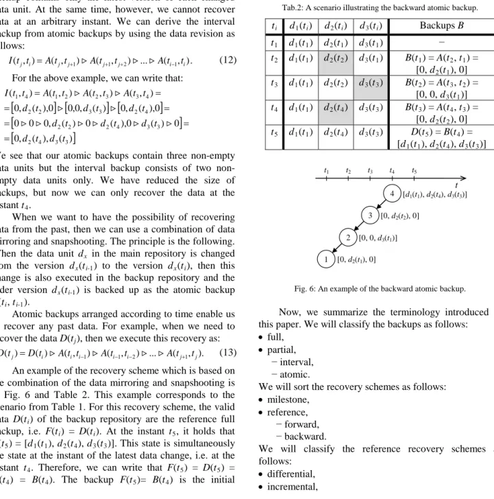
An example of the recovery scheme which is based on the combination of the data mirroring and snapshooting is in Fig. 6 and Table 2. This example corresponds to the scenario from Table 1. For this recovery scheme, the valid data D(ti) of the backup repository are the reference full
backup, i.e. F(ti) = D(ti). At the instant t5, it holds that
F(t5) = [d1(t1), d2(t4), d3(t3)]. This state is simultaneously the state at the instant of the latest data change, i.e. at the instant t4. Therefore, we can write that F(t5) = D(t5) =
D(t4) = B(t4). The backup F(t5)= B(t4) is the initial
reference backup for the incremental recovery scheme with subsequent atomic backups A(t4, t3) = [0, d2(t2), 0], A(t3,
t2) = [0, 0, d3(t1)], and A(t2, t1) = [0, d2(t1), 0].
Let us note that this scheme is very similar to the atomic incremental scheme in Fig. 5. The difference between these schemes is their orientation in time. In Fig. 5, we see the forward incremental scheme while Fig. 6 illustrates the backward incremental scheme. We point out that the backward recovery schemes need not be incremental atomic schemes only. As we mentioned above, we can derive arbitrary interval backups from atomic backups by using (12). This enables us to construct arbitrary backward interval schemes.
Tab.2: A scenario illustrating the backward atomic backup.
ti d1(ti) d2(ti) d3(ti) Backups B t1 d1(t1) d2(t1) d3(t1) − t2 d1(t1) d2(t2) d3(t1) B(t1) = A(t2, t1) = [0, d2(t1), 0] t3 d1(t1) d2(t2) d3(t3) B(t2) = A(t3, t2) = [0, 0, d3(t1)] t4 d1(t1) d2(t4) d3(t3) B(t3) = A(t4, t3) = [0, d2(t2), 0] t5 d1(t1) d2(t4) d3(t3) D(t5) = B(t4) = [d1(t1), d2(t4), d3(t3)] 1 2 3 t1 t2 t3 t4 t5 t [d1(t1), d2(t4), d3(t3)] [0, d2(t2), 0] [0, 0, d3(t1)] [0, d2(t1), 0] 4
Fig. 6: An example of the backward atomic backup.
Now, we summarize the terminology introduced in this paper. We will classify the backups as follows:
•full,
•partial, − interval, − atomic.
We will sort the recovery schemes as follows:
•milestone,
•reference, − forward, − backward.
We will classify the reference recovery schemes as follows:
•differential,
• combined.
In the next section, we introduce a mathematical model for a quantitative evaluation of backups and recovery schemes.
5. Mathematical model
In this section, we deal with a mathematical model which enables us to quantify the size of different backups. This enables us to evaluate the properties of different data recovery schemes. We derive the model for the forward recovery schemes, but the formulas obtained are also valid for the backwards recovery schemes. In the model, we assume that all data units dx consist of the same number of
symbols. We will call this number of symbols the size of the data unit and denote it by |d|. We pessimistically suppose that there are no empty data units in the main repository, i.e. all n data units always contain certain data. Then, for the total amount of the data |D| stored in the main repository, it holds that |D|= n⋅|d|. The same formula evidently holds for the size of the full backup:
. ) (t D
F i = (14)
Now, let us solve the size of partial backups. Let us suppose that the (i−1)-th change of the data unit dx
occurred at the instant ti- 1 and the i-th change of this data unit occurred at the instant ti. Denote the time between
these consecutive changes by ui, i.e. ui = (ti− ti- 1). In the model, the times ui are represented by the random variable U whose averaged value is Δ. We assume that this averaged value is the same for all data units. Then, the variable λ = 1/Δ represents the rate of changes of each data unit. We further assume that the probability distribution of the random variable U is an exponential distribution. The cumulative distribution function G of this distribution is:
. 1 ) Pr( ) (u U u e λu G = ≤ = − − (15)
Now, we will represent mathematically the interval backups. To this purpose, we will use the quantities in Fig. 7. In the Figure, the instants t1, t2, t3, and t4 are indicated. The instants t1 and t4 are instants at which a certain data unit was changed. The instants t2 and t3 are instants at which the data backup was executed. We note that these backups need not be adjacent. The quantity τ = (t3− t2) is the time between these backups, the variable u = (t4− t1) is the time between two consecutive changes of the data unit (i.e. a realization of the random variable U), and the quantity r = (t2− t1) is the time between the change of the data unit and the following backup.
Now, we are interested in the probability Q(τ), which is the probability that when the data unit has not been again changed until the first backup (i.e. until t2), then this data unit is not changed until the instant of the next observed
backup (i.e. until t3 = t2 + τ). We can formally express this probability as a conditional probability:
. ) Pr( ) (τ U r τ U r Q = > + > (16)
Fig.7: Quantities for the derivation of the mathematical model.
The exponential distribution is a distribution without memory and therefore it holds (e.g. [11], p. 40):
. ) Pr( )
Pr(U>r+τ U>r = U>τ (17) It follows from (17) that when the data unit is not changed in the time interval r (the condition U > r), then the probability that this data unit does not change in the time interval (r + τ) is the same as the probability that this change does not occur in the time interval τ. Then we have:
. ) ( 1 ) Pr( 1 ) Pr( ) Pr( ) ( λτ e τ G τ U τ U r U τ r U τ Q − = − = ≤ − = = > = > + > = (18) The complementary probability P(τ) = 1 − Q(τ) is, of course, a probability that the data unit is changed in the time interval τ. The data D consist of n data units and therefore the interval backup I(ti − τ, ti) on average
consists of n⋅P(τ) changed data units. Then the average size |I(ti− τ, ti)| of this backup is:
(
1)
. ) ( ) , (ti τ ti d n P τ D e λτ I − = ⋅ ⋅ = ⋅ − − (19)This formula enables computing the average size of each subsequent interval backup B(ti) = I(ti− τ, ti), which
is spaced the time interval τ from its reference backup B(ti
− τ).
Let us assume that backups are executed periodically with the time interval T. Then it holds that the time interval between two different backups τ = k⋅T, where k = 1, 2, 3, ....
Now, let us define the quantity q:
. ) (T e λT Q
q= = − (20)
The quantity q is the probability that the data unit does not change in the time interval T. The quantity p = 1−q is the probability that the data unit changes in the time interval T. For this quantity, it holds:
. 1 1 q e λT
p= − = − − (21)
Then the average size of the interval backup I(ti− k⋅T, ti) is:
(
1)
(
1)
. ) , ( λkT k i i k T t D e D q t I − ⋅ = ⋅ − − = ⋅ − (22) t1 t2 t3 t4 t r τ uThis formula enables computing the average size of each subsequent interval backup B(ti) = I(ti − k⋅T, ti),
which is spaced the time interval k⋅T from its reference backup B(ti− k⋅T).
Now, we determine the total average size S of the aggregate of atomic backups from the time interval T. We have already introduced the notation according to which the rate of changes of each data unit is λ and the number of data units is n. Then, the total number of changes N = n⋅λ⋅T. Each such change is recorded in one atomic backup of |d| symbols in size. Therefore, the total average size |S(ti− T, ti)| of the aggregate of atomic backups from the time
interval T is: . 1 1 ln ) , ( p D T λ D T λ n d t T t S i i − ⋅ = ⋅ ⋅ = ⋅ ⋅ ⋅ = − (23)
We note that the inversion of equation (21) was used to express |S(ti− T, ti)| in the latest term.
By using formulas (14), (22), and (23), we can quantify the average size of different types of backup. Now, we can quantitatively analyze the different types of recovery scheme.
6. Discussion
We will illustrate the utilization of our model on recovery schemes in Figs 1 to 4. The milestone scheme is in Fig. 2, the differential scheme in Fig. 3, the incremental scheme in Fig. 4, and the combined scheme in Fig. 1. We note that the schemes introduced are comparable since all these schemes consist of M = 5 backups. We will restrict ourselves to forward schemes only, but the results obtained, of course, also hold for the equivalent backward recovery schemes. With all interval recovery schemes, we assume that the backups are executed with the period T. The size of the data D(ti) and the backups B(ti) will be denoted
|D(ti)| and |B(ti)|, respectively.
For a comparison of the schemes, we will utilize two parameters. The first parameter is the average total backup size C. We compute the value of this parameter by summing the average sizes of all backups in the given scheme, i.e.: . ) ( 1
∑
= = M i i t B C (24)The parameter C represents the storage space demands of the given recovery scheme and therefore we try to minimize its value. A higher value of the average total backup size means the backup repository has a larger storage capacity and therefore a higher cost too.
The average recovery time is the next criterion for evaluating the recovery schemes. If we assume a constant rate of writing data from the backup repository into the main repository, then the average recovery time depends
on the average size of backups that we must write into the main repository in order to recover the required data D(ti). However, to recover different data, i.e. D(t1) to D(tM),
we must write into the repository the different backups of different sizes. For example, in the recovery scheme according to Fig. 1, we need to write only the full backup
B(t1) to recover the data D(t1). However, to recover the data D(t5), we need to write into the repository the backups
B(t1), B(t4), and B(t5). We will call the set of backups needed for recovering the data D(ti) the recovery data and
denote their average size by Ri. Now, let us return to the
recovery schemes. We recall that the node i represents the backup at the instant ti. We will call the node of a full backup the root. Let us denote by Vi the set of nodes in the
path from the root to the node i. In our example, the path for the node 1 is given by the node 1 itself and therefore V1 = {1}. In the case of the node 5, the path is given by the sequence of nodes 1-4-5 and therefore V5 = {1, 4, 5}. Then, for Ri it holds: . ) (
∑
∈ = i V k k i Bt R (25)For example, according to Fig. 1, R5 = |B(t1)| + |B(t4)| + |B(t5)|. By using (25), we can compute the size of the data for recovering any state of D(ti). We will call the
average value of all quantities R1 to RM the average data
recovery size and denote it by R. Formally, we can write: . 1 1
∑
= ⋅ = M i i R M R (26)The average recovery time depends in direct proportion on the quantity R and therefore we try to minimize the value of R. In such a case, the data recovery will be the fastest on average.
Now, we derive the formulas for C and R for all the schemes considered. In the case of the milestone scheme (Fig. 2), we see that the average total backup size equals the sum of the average sizes of all M = 5 full backups, i.e. it holds: . ) ( 1 M D t F C M i i = ⋅ =
∑
= (27)The average sizes of the recovery data Ri are identical
for all D(ti), where Ri = |D|. Therefore, for the average
data recovery size R, it simply holds:
.
D
R= (28)
In the case of the differential recovery scheme (see Fig. 3), we know that B(t1) = F(t1) and B(ti) = I(t1, ti),
where i = 2 to M. Then for the sizes of single backups, it is valid: = − ⋅ = = = = − . ,... 3 , 2 ), 1 ( ) , ( , 1 , ) ( ) ( 1 1 1 M i q D t t I i D t F t B i i i (29)
By substituting these quantities into (24), (25), and (26), we finally obtain: − − − ⋅ = q q q M D C M 1 (30) and . 1 1 2 − − − − ⋅ ⋅ = q q q M M D R M (31) In the case of the incremental recovery scheme (see Fig. 4), we know that B(t1) = F(t1) and B(ti) = I(ti− 1, ti),
where i = 2 to M. Then for the sizes of single backups, it is valid: = − ⋅ = = = = −, ) (1 ), 2,3,... . ( , 1 , ) ( ) ( 1 1 M i q D t t I i D t F t B i i i (32)
By substituting these quantities into (24), (25), and (26), we finally obtain:
(
)
[
M M q]
D C= ⋅ − −1⋅ (33) and(
)
[
1 1]
. 2 M M q D R= ⋅ + − − ⋅ (34)For comparison, we additionally derive the quantities
C and R for the combined recovery scheme in Fig. 1. The first backup is full, i.e. |B(t1)|= |D|. The second, third and fifth backups are spaced one time interval T from their reference backups and therefore we can write that |B(t2)| = |B(t3)| = |B(t5)| = |D|⋅(1 − q). The fourth backup is spaced the time interval 3⋅T from its reference backup and therefore |B(t4)| = |D| ⋅ (1 − q3). By substituting these quantities into (24), (25), and (26), we obtain:
(
3)
3 5 q q D C= ⋅ − ⋅ − (35) and(
11 4 2)
. 5 3 q q D R= ⋅ − ⋅ − ⋅ (36)To compare C and R for the schemes considered, we utilize the functions C = f(p) and R = g(p), where p is the probability that the data unit is changed in the time interval
T. The graphs of functions C = f(p) in the multiples of the quantity |D| are in Fig. 8 for the all schemes considered. In the case of the milestone recovery scheme, the value of C
is the constant 5⋅|D| or generally M⋅|D|.
Now, let us analyze the reference recovery schemes. For p = 0, we can see that C = |D| for all reference schemes. This is due to the fact that there are no changes in the data units. All subsequent backups are empty and the value C = |D| is given by the first (i.e. full) backup. The second common extreme of all reference schemes is the value of C
when the rate of data unit changes λ → ∞. In this case, all data units are always changed within the interval T and
therefore the probability p = 1. Then, the total average size
C of backups equals the value M⋅|D|, i.e. the storage space demands of all reference schemes are identical with those of the milestone scheme.
0.2 0.4 0.6 0.8 0 1 0 C 1 2 3 4 5 p Milestone Differential Combined Incremental [|D|]
Fig. 8: The dependence of the average total backup size
C on the probability p for different recovery schemes. When we compare all schemes, we can see that there are two extremes. The first extreme is the milestone recovery scheme. For all p ∈ (0, 1), this scheme has the highest demands on the storage capacity of the backup repository. The second extreme is the incremental recovery scheme where, by contrast, these storage space demands are the lowest. Then, we can take the storage space demands of the milestone recovery scheme as an upper bound:
M D
Cmax= ⋅ (37)
and the storage space demands of the incremental recovery scheme as a lower bound:
(
)
[
1 1]
min= D⋅ M− ⋅p+
C (38)
The storage space demands of the other schemes are between these bounds.
Fig. 9 illustrates the functions R = g(p), i.e. the dependence of the average data recovery size R on the probability p. We can see that the lower bound of R is given by the milestone recovery scheme:
.
min D
R = (39)
By contrast, the upper bound of R is given by the incremental recovery scheme:
. 1 2 1 max − ⋅ + ⋅ = D M p R (40)
From the two figures above, we can see that the milestone and incremental recovery schemes are boundary cases for both the quantity C and the quantity R. The milestone recovery scheme is the worst scheme from the viewpoint of storage space demands, but the best scheme from the viewpoint of the recovery time. In the case of the
incremental recovery scheme, the exact opposite holds. Then, we can take the differential scheme and combined recovery schemes as a compromise between the two extremes above. 0 0.2 0.4 0.6 0.8 1 0 0.5 1 1.5 2 2.5 3 Incremental R p Milestone Differential [|D|] Combined
Fig. 9: The dependence of the average data recovery size R on the probability p for different recovery schemes.
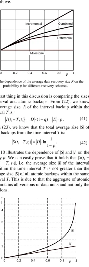
The last thing in this discussion is comparing the sizes of the interval and atomic backups. From (22), we know that the average size |I| of the interval backup within the time interval T is:
. ) 1 ( ) , (t T t D q D p I i− i = ⋅ − = ⋅ (41)
From (23), we know that the total average size |S| of all atomic backups from the time interval T is:
. 1 1 ln ) , ( p D t T t S i i − ⋅ = − (42)
Fig. 10 illustrates the dependence of |S| and |I| on the probability p. We can easily prove that it holds that |S(ti − T, ti)|/|I(ti − T, ti)|, i.e. the average size |I| of the interval
backup within the time interval T is not greater than the total average size |S| of all atomic backups within the same time interval T. This is due to that the aggregate of atomic backups contains all versions of data units and not only the latest versions. 0 0.2 0.4 0.6 0.8 1 0 1 2 3 4 5 |S|, | I| p |S| |I| [|D|]
Fig. 10: Dependence of |S| and |I| on the probability p.
From the Figure, we can see that the differences between |S| and |I| are not significant for small values of p. However, these differences are definitely significant for greater values of p. For example, the ratio |S| / |I| equals approximately 1.4 for p = 0.5. Then, in the case of the atomic backup, we need a backup repository with a capacity which is 40 percent greater than in the case of the interval backup. In the case of p ≈ 0.8, the ratio |S| / |I| equals 2, i.e. we need a backup repository with a capacity which is two times greater than in the case of the interval backup. The advantage of the atomic backup, i.e. the possibility of recovering the data at any time instant, is paid for by increased requirements for the storage capacity of the backup repository.
7. Conclusion
In the paper, the terminology and mathematical apparatus for data backup and recovery is extended. The core of the paper is a mathematical model of the data backup and recovery. The mathematical model enables us to compute the average size of an arbitrary backup (eq. 21 and 22) from the probability p that the data unit is changed in the time interval T. It enables us to determine the average total backup size C (eq. 24) for any recovery scheme and also the average data recovery size R (eq. 26). The model proposed allows us to compare different recovery schemes (e.g. Fig. 8 and 9) and extends the theory of the data backup and recovery. The model also allows us to compare interval and atomic backups (see eq. 22, 23 and Fig. 10).
The model introduced is based on the assumptions that the probability p is the same for all data units and that the data unit change is an event which has no influence on the changes of other data units, i.e. these changes are mutually independent events. Further assumptions are that the total size of the data is constant and that no data unit is empty. The assumptions introduced are not general and therefore our next goal is to create a more general model. In any case, however, the model described is suitable for theoretic purposes at least.
References
[1] A. Frisch: System Backup: Methodologies, Algorithms and
Efficiency Models. In J. Bergstra, M. Burgess: Handbook of
Network and System Administration. Elsevier, Amsterdam 2007.
[2] S. Nelson: Pro Data Backup and Recovery. Apress, New
York 2011.
[3] A. Frisch: Essential System Administration. O’Reilly Media,
[4] Z. Kurmas, A. L. Chervenak: Evaluating Backup Algorithms. In IEEE Symposium on Mass Storage Systems. 2000, pp. 235-242.
[5] M. Burgess, T. Reitan: A risk analysis of disk backup or
repository maintenance. Science of Computer Programming. 64 (2007), pp. 312-331. DOI: 10.1016/j.scico.2006.06.003.
[6] C. Qian, Y. Huang, X. Zhao, Toshio Nakagawa: X: Optimal
Backup Interval for a Database System with Full and Periodic Incremental Backup. Journal of Computers. 5 (2010), pp. 557-564.
[7] Teradactyl: Backup Terms and Definitions. Teradactyl LLC.
Retrieved April 17, 2014 from
http://www.teradactyl.com/backup-knowledge/backup-definitions/backup terminology.html
[8] N. Garrimella: Understanding and exploiting snapshot
technology for data protection. Part 1: Snapshot technology overview. IBM developerWorks. (April 26, 2006). Retrieved April 17, 2014 from
http://www.ibm.com/developerworks/tivoli/library/t-snaptsm1/index.html?ca=dat-
[9] P. de Guise: Enterprise Systems Backup and Recovery.
CRC Press, Boca Raton 2008.
[10]M. Liotine: Mission-Critical Network Planning. Artech
House, London 2003.
[11]L. Lakatos, L. Szeidl, M. Telek: Introduction to Queueing
Systems with Telecommunication Applications. Springer, New York 2013.
Karel Burda received the M.S. and PhD. degrees in Electrical Engineering from the Liptovsky Mikulas Military Academy in 1981 and 1988, respectively. During 1988-2004, he was a lecturer in two military academies. At present, he works at Brno University of Technology. His current research interests include the security of information systems and cryptology.