A cluster based collaborative filtering method for improving the performance of recommender systems in ecommerce

i

A thesis submitted in partial fulfilment of the requirements for the

degree of Master of Computing

A Cluster Based Collaborative Filtering Method for Improving

the Performance of Recommender Systems in Ecommerce

By

Alaa Alahmadi

1355154

Supervisor: Dr. Bahman Sarrafpour (Sassani)

Associate Supervisor: Dr. Hamid Sharifzadeh

Unitec Institute of Technology

2017

ii

Abstract

Rapid growth of E-commerce has made a huge number of products and services accessible to the users. The vast variety of options makes it difficult for the users to finalize their decisions. Recommender systems aim at offering the most suitable items to the users. To do this, recommender systems use data about user’s behaviour and interest (in the past) and characteristics of items. In addition to the data, recommender systems employ machine learning algorithms to build sophisticated models to predict the user’s behaviour in the future.

In this thesis, two new methods are proposed for recommender systems both of which consist of two phases: offline and online. In the offline phase, users are clustered based on their similarities; and in the online phase, items which are interesting for a user’s cluster members are recommended to that user.

The first proposed method, CFGA, is based on collaborative filtering technique, uses genetic algorithm to cluster users in the offline phase. The fitness function takes into account the users’ ratings and rating times. In the online phase, the ratings of the target user for each item is calculated from the ratings of his or her cluster members to that item. Items with ratings above a threshold are considered interesting for the user and are recommended to him or her. The method is evaluated with two data sets from Movielens for which experimental results show that CFGA is more accurate than several existing recommendation methods. However, there are a couple of existing methods that outperform CFGA.

The second method is a hybrid method which combines collaborative filtering and demographic recommendation algorithms. Similarly to CFGA, the second method uses genetic algorithm for clustering users. However, the fitness function, in addition to users’ ratings, incorporates demographic information about users (age, occupation, and sex). Experimental results show that the hybrid method outperforms not only CFGA, but also all existing similar methods.

iii

Acknowledgements

The completion of this thesis is largely due to the assistance of many people and organizations. I would like to thank each of them individually.

First of all, I must thank Allah Almighty for his blessings, kindness and help not only for completing this thesis and my studies but also for my whole life.

Then, I must thank Saudi Culture Mission for providing me a scholarship and supporting me throughout my stay in New Zealand.

I would like to thank my experienced supervisor, Dr Bahman Sarrafpour, for his great personality and deep knowledge. My deepest thanks to him for his thoughtful guidance during my masters and his patience, help and extremely valuable comments for writing this thesis.

I would also thank my associate supervisor Dr Hamid Sharifzadeh for reviewing my thesis and providing me useful feedback.

Last but not least, my special thanks to all my friends for their support and help.

Alaa Alahmadi Unitec

iv

1

Table of Contents

2 Chapter 2: Literature Review ... 4

2.1 Definitions ... 5

2.2 Recommender Systems ... 5

2.3 Collaborative Filtering (CF) ... 5

2.4 Content Based Filtering ... 13

2.5 Knowledge Based Recommender Systems ... 14

2.6 Demographic Recommender System ... 16

2.7 Hybrid Recommender Systems ... 16

2.8 Context-aware Recommender Systems ... 17

2.9 Cross-Domain Recommender Systems ... 17

2.10 Bio-inspired Approaches ... 18

2.11 Summary ... 20

3 Chapter 3: The CFGA Method ... 22

3.1 Offline Phase ... 23

3.2 Online phase ... 26

3.3 Evaluation... 27

3.4 Summary ... 32

4 Chapter 4: The Hybrid Method ... 33

4.1 Offline Phase ... 34

4.2 Online Phase ... 36

4.3 Evaluation... 36

4.4 Summary ... 38

5 Chapter 5: Conclusions and Future Work ... 40

5.1 Summary ... 41

5.2 Future Work ... 42

vi

List of Figures

Figure 2-1. A user-item matrix and its corresponding graph ... 9

Figure 2-2. Term frequency indexing (Mortensen, 2007) ... 14

Figure 2-3. An architecture of constraint-based recommender systems (Zanker, Aschinger, & Jessenitschnig, 2010) ... 15

Figure 2-4. Demographic-based approach (Safoury & Salah, 2013) ... 16

Figure 3-1. MAE of the CFGA method (dataset 1) ... 29

Figure 3-2. Accuracy of the CFGA method (dataset 1) ... 29

Figure 3-3. Comparison of CFGA and the previous methods in terms of MAE (dataset 1)... 30

Figure 3-4. Comparison of CFGA and the previous methods in terms of Accuracy (dataset 1) ... 30

Figure 3-5. Comparison of CFGA and the previous methods in terms of MAE (dataset 2)... 31

Figure 3-6. Comparison of CFGA and the previous methods in terms of Accuracy (dataset 2) ... 31

Figure 4-1. Comparing the MAE of the proposed methods (dataset 1) ... 36

Figure 4-2. Comparing the accuracy of the proposed methods (dataset 1) ... 37

Figure 4-3. Comparing the proposed methods and the previous methods (dataset 1) ... 37

Figure 4-4. Comparing the accuracy of the proposed methods and previous methods (dataset 1) ... 37

Figure 4-5. Comparing the MAE of the proposed methods and previous methods (dataset 2) ... 38

vii

List of Tables

1

2

“We have 6.2 million customers; we should have 6.2 million stores. There should be the optimum store for each and every customer.”

—Jeff Bezos, founder and CEO of Amazon.com in an interview for Business Week during March 1999.

In recent years, E-commerce has experienced a significant rise in number of trades and users. A vast stream of information has been produced by the websites of companies advertising their products. Digestion of this huge amount of information is impossible for buyers. Recommender systems aim at filtering the enormous quantity of available information to find interesting information for users (Benshafer, Konstan, & Riedl, 1999). There are many recommender systems available. Here are three famous examples:

 Youtube uses a recommender system to suggest videos to its users based on their previously watched videos.

 Amazon provides a recommended list of its new publications for its customers based on their previously purchased books.

 Facebook uses a recommender system to recommend new friends to the users.

Recommender systems use the existing data about users, items, and the interaction of users. Then apply various machine learning algorithms to build models which predict the future behaviour of users in the system. In this way, recommender systems predict which items may be interesting for users to be recommended to them.

One of the most popular methods for implementing recommender systems is collaborative filtering (CF) which takes into account users’ ratings to calculate their similarity. Then, a user’s rating to an item is calculated from the ratings of similar users to this item. Items with a rating more than a threshold are recommended to the user.

Another type of recommender systems use demographic information of users to determine their similarity. These systems are called demographic recommender systems. Demographic recommender systems use a list of items that have good feedback from similar users to recommend to the target user.

1.1

Problem Statement

Collaborative filtering (CF) algorithms use previous interactions of the users with the system. These interactions construct the user’s profile which can be used to determine his or her neighbourhood (i.e., those users who are similar to him or her). CF algorithms rely to this general fact that users who have had similar behaviour so far, will have similar behaviour in the future. Determining the user’s neighbourhood effectively is a big challenge in CF algorithms which impacts their accuracy. One of the effective methods to group similar users together is clustering. To predict the behaviour of a user, the behaviour of the users in the same cluster is considered. A good clustering algorithm results in high accurate recommendations.

In this thesis, two recommendation methods are proposed both of which consist of two phases: offline and online. In the offline phase, users are clustered and in the online phase their ratings to unrated items are predicted. Both methods use genetic algorithm (GA) in the offline phase to minimize the inter-cluster distances. The first method, Collaborative Filtering Generic Algorithm (CFGA), is based on collaborative filtering technique and determines users’ similarity based on

3

their ratings and rating times. The second method is a hybrid method which combines collaborative filtering and demographic algorithms. In addition to users’ ratings and rating times, it uses users’ personal information in the similarity function.

1.2

Thesis Overview

The rest of the thesis is organized as follows:

Chapter 2 reviews basic concepts of recommender systems and some of the existing recommender systems that are similar to this research.

Chapter 3 details the concept of CFGA method and detailed evaluation of CFGA methodology. Chapter 4 explains the motivation to improve CFGA and the idea of the hybrid method. Then, the hybrid method is evaluated and compared with CFGA and with similar exiting methods.

Finally, Chapter 5 concludes the thesis along with future directions for the research.

1.3

Research Contribution

CF is the mostly researched and widely used recommender system that applications use. However, CF has significant drawbacks that affect the accuracy of recommendations. Hence this research is focused to develop CF in two steps, improve to CFGA and then to hybrid models.

1.4

Research Methodology

To determine the accuracy of the recommender system it is paramount to have large amount of data with user preferences and demographics. Furthermore, it is required to have large amount of items that users to tag their preferences. Hence it was vital to have real user data rather than simulated or any other system generated data for more accurate analysis in this research. The Movielens provides their survey and user preferences for the research purposes. Hence this research is conducted by analysing data that has been obtained by Movielens. The number of users (sample size) is a limitation that researcher that have no control. However, the databases contains close to 1000 user data which is more than adequate for statistical analysis.

4

5

This chapter includes basic concepts which are necessary for the reader to better understand the thesis. Then, similar researches are reviewed.

2.1

Definitions

- Item: Item refers to the things in the system that are recommended to the users. These

could be movies, books, songs, or any other product or service.

- Target User: The target user (or active user) is the user who is considered for

recommendation by the system.

- Rating: It shows how much a user is interested to an item. Rating can be either explicit

(e.g. a user rates a movie as 5 out of 5 which shows the user is really interested in watching the movie) or implicit (e.g., the user watches a movie several times which indicates the user is interested in that movie). For example, the music streaming website, last.fm uses implicit information such as number of times a user listen to a particular song to rate that song.

- Accuracy: It shows how many of the recommended items to the users are really

interesting for them. Accuracy is one of the most crucial factors in evaluating new recommender systems. Recommender systems with low accuracy not only cannot absorb new customers, but also may lose current customers. When customers receive many emails from a website advertising uninteresting products, they may ignore all emails or even block the email address.

2.2

Recommender Systems

There has been a lot of research conducted on recommender systems. In this chapter, I review some of the published research similar to my research. Current recommender systems fall into different categories as follows (Aggarwal, 2016):

- Collaborative filtering (CF)

- Content based recommender systems - Knowledge based recommender systems - Demographic recommender systems - Hybrid recommender systems

- Context-aware recommender systems - Cross-domain recommender systems - Bio-inspired approaches

These categories will be detailed in the following sections.

2.3

Collaborative Filtering (CF)

Collaborative filtering systems typically take the user’s long term profile into account in which meta data about his or her interests such as feedback and preferences can be found (Rafeh & Bahremand, 2012). This kind of feedback or interests may be implicit or explicit. Users’ similarities are the basis of recommendation in CF systems. For example, a movie recommendation system based on collaborative filtering can use users’ profiles to find a group of users with similar preferences. Then, when one of these users watches a movie, the movie is recommended to the other users in that group.

6

CF recommender systems usually use a user-item matrix X which has K rows and M columns for K users and M items. Xij shows the rate of user i to item j.

𝑋 = [

𝑥_1,1 ⋯ 𝑥_1,𝑀

⋮ ⋱ ⋮

𝑥_𝐾,1 ⋯ 𝑥_𝐾,𝑀]

This matrix can be decomposed into row vectors as follows: X = [u1,...,uK], ui = [xi,1,...,xi,M],i = 1,...,K

Each row vector ui corresponds to a user profile and represents the ratings of that user.

The matrix can also be represented by its column vectors: X = [v1,...,vM],vj = [x1,j,...,xK,j],i = 1,...,M

Each column vector vj shows how users rated item j.

CF systems are themselves classified into two groups (Su & Khoshgoftaar, 2009):

- Memory based - Model based

These are explained in the next two sections.

2.3.1

Memory-Based Collaborative Filtering Techniques

Memory based algorithms predict the ratings of the active user based on his or her similar users’ ratings (Linden, Smith, & York, 2003). These algorithms use the entire or a sample of the user-item database for prediction. One of the most popular memory-based CF techniques is the K-Nearest Neighbour (KNN) technique in which similar users are grouped together. The group members are also called neighbours. The prediction of a new user’s (or active user’s) rating for an item is based on his or her neighbours’ rates to the same item. So, the neighbourhood-based CF algorithm consists of the following steps:

a. Calculate the similarity of two users or two items:

There is a lot of research conducted on finding the set of k users similar to the active user u (i.e., the user who will be recommended by the system) in collaborative filtering. The set of k most similar users to the active user forms the active user’s neighbourhood. Similarity between two users determines how their behaviours may be similar in the future. The quality of the similarity function has a major impact on the accuracy of prediction. The most common similarity functions are as follows.

 Pearson Correlation Coefficient Similarity

Pearson Correlation Coefficient (PCC) is the most widely used metric for similarity calculation. It calculates the similarity between users based on their ratings to items. Equation

(2-1) defines similarity between two users u and v in which is the mean rating for user u, is the rating of user u to item i and I is the set of common items rated by both users u and v (Resnick, Iacovou, Suchak, Bergstrom, & Riedl, 1994).

u

7

(2-1)  Cosine Similarity

Cosine similarity function is another popular metric which measures the similarity of two users by considering their rates for commonly rated items as two vectors and finding the cosine of the angle between these two vectors (Sarwar, Karypis, Konstan, & Riedl, 2000). This is shown in Equation (2-2):

(2-2)  Jaccard Similarity

Jaccard metric is one of the simplest approaches in measuring similarity between two users. It considers common items rated by both users regardless of the rates they have received from users (Charikar, 2002). Jaccard metric is useful when there is no reliable rating available for items. This metric is shown in Equation (2-3).

(2-3) b. Produce a prediction for the active user by calculating the weighted average of all the

ratings in his/her neighbourhood

The most crucial part of a collaborative filtering algorithm is determining recommendation for the active user. After finding the active user’s neighbourhood, Equation (2-4) is used to aggregate the rates and to predict the rate of user u to item i (Resnick, Iacovou, Suchak, Bergstrom, & Riedl, 1994): (2-4)

















8

In most of collaborative filtering methods, Pearson coefficient and cosine-based methods are used to obtain the amount of similarity between two users. In (Dakhel & Mahdavi, 2013) a collaborative filtering technique has been proposed in which the distance between users is calculated using seven different methods (i.e., Euclidean distance, Chebyshev distance, Gaur distance, Sorensen distance, Canberra distance, distance and Lorentzian and City block distance). KNN and K-Means have been used to determine the most similar users to the active user. After determining the active user’s neighbours, the system predicts the user’s rate for the items that are not yet rated as follows:

User’s rate for item i = the most popular rate (rate of majority) that the neighbours have given to item i.

For example, if the rating range is from A to E and 60% of the user’s neighbours give rate E to the desired item, rate E is considered for the active user too. They have tested their proposed approach on the Movielens dataset and found K-Means with Euclidian distance the most appropriate method for Movielens.

2.3.2

Model-Based Collaborative Filtering Techniques

Model-based CF techniques use a dataset to build a descriptive model of users, items and ratings. The model construction can be built off-line and may take several hours or days. Then, the model is used for recommendations.

Bayesian clustering is one of the statistical approaches to construct a model. Users are grouped using their preferences. Then, based on the membership of the active user to one of these clusters, his or her rating for a given item would be calculated. The number of clusters and the model parameters are learned from the dataset. Bayesian networks is another common statistical approach to construct the model where each node in the network represents an item in the dataset. The state of each node shows the possible rating for that item. The structure of the network and the conditional probabilities are learned from the dataset.

Rule-based approaches can be also used for constructing models where association rules discover the associations between co-purchased items. Then, recommendations are generated based on the strength of the association between items (Mortensen, 2007).

Model-based CF systems have several advantages over memory-based CF systems as follows:

- Model-based approaches may find certain correlations in the data and hence may offer

added values beyond their predictive capabilities.

- Model-based systems need less memory than memory-based systems.

- Model-based systems generate predictions quickly once the model is generated.

2.3.3

Challenges with Collaborative Filtering Approaches

Collaborative filtering systems are easy to implement and to add new information. However, they suffer from three problems:

- Cold-start problem which means recommendation for a new user could be inaccurate

because there is no history about him or her. This is also true for new items.

- Sparsity which means the user-item matrix is sparse. This happens when there is no

9

system for apartment purchase it is impossible to collect enough information about the users to build their profiles because people do not buy apartments frequently.

- Scalability which means when the number of users and items grow, storing and handling

the user-item matrix becomes a challenge.

2.3.4

Incorporating the Time Factor in Collaborative Filtering

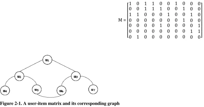
Users’ needs may change over time, and this is what has been neglected by most of the algorithms. This means that the similarity of two users may change over time. In fact, the users’ last interactions with the system are more important than their interactions performed a long time ago. In (Rafeh & Bahremand, 2012) a time-based collaborative filtering algorithm is presented which considers the time factor in the similarity function. The proposed method consists of the following steps:

- Creating item-user graphs - Calculating weights of edges - Measuring the similarities of users

- Recommending the active user based on the calculated similarities

Figure 2-1 shows a sample user-item matrix and its corresponding graph in which nodes represent users and the links show the two users have at least one common item rated. For example, in matrix M, users are represented in row and columns could be 10 different movies. Furthermore, 1 represent user likes the movie and 0 represent user doesn’t like the movie.

M = [ 1 0 1 1 0 0 1 0 0 0 0 0 1 1 1 0 0 0 0 1 1 0 0 0 1 0 0 0 0 1 0 0 0 0 1 0 0 1 0 0 0 0 0 0 0 0 0 1 0 0 1 0 0 0 0 0 0 0 0 0 0 1 0 0 1 1 0 0 0 0]

Figure 2-1. A user-item matrix and its corresponding graph

To calculate the similarity of two neighbouring users u and v in the graph (i.e., two nodes with a direct link) the following formulas are being used:

10 1 (2-5) 2 (2-6) 3 (2-7)

The above formulas calculate the sum of rate difference, time difference and priority difference, respectively. CI represents the set of items commonly rated by u and v, Ru,i and Tu,i indicate the

rate of user u for item i and the time u has rated i, respectively. The list of items rated by each user is sorted on the rating time descending. In Equation (2-7), Pu,i shows the priority of item i in the

rating list of user u.

Then, the rate difference and the priority difference are normalized using the following equation:

(2-8)

(2-9)

(2-10)

Where represents the number of items commonly rated by u and v and MCIu,v indicates the

number of all possible items commonly rated by u and v. MRateDiffu,v is the maximum rate

1 _{Sum of Rate Differences}

2 _{Sum of Time Differences} 3 _{Sum of Priority Differences}







11

difference between u and v. The following equation calculates MRateDiffu,v for an n-star feedback

system:

(2-11)

The maximum dissimilarity between the active user’s interaction sequence and another user’s sequence is calculated using the following equation:

MSOPD(n) =

An adaptive decay function is used to use SOTDu,v as follows:

(2-13)

The following equation incorporates the time factor for the similarity of two direct neighbours:

(2-14)

The similarity of two direct neighbours regardless of the time factor is measured by the following equation:

(2-15)

u oportion _MaxRateDifSORD _f

12

Where EOR is a factor that influences the BaseWeight and EOT is another factor to show the influence of the time factor on the similarity of two direct neighbours.

Finally, the following equation calculates the weight (similarity) between two neighbouring users u and v, which is a number in the range [0,1] where 1 means the maximum similarity.

(2-16)

After calculating the weight of adjacent nodes in the graph, the similarity of the active user with his or her indirect neighbour is calculated by multiplying the weight of the links in the path between them.

In the final stage, the rates of the active user u to item i is calculated using the following formula:

(2-17)

Where and are the mean ratings of users u and v for all rated items, respectively; U is the set of similar users to u; Simu,v is the similarity between u and v. TimeImpact(v,i) indicates the time

of rating and is calculated using the following formula:

(2-18)

The method has been evaluated using Movielens and Amazon datasets and the results show that the proposed method outperforms the traditional CF approach for both datasets.

2.3.5

Incorporating the Location Factor in Collaborative Filtering

In (Levandoski, Sarwat, Eldawy, & Mokbel, 2012) another factor is considered for recommendation: location. The proposed recommender system named LARS (Location-Aware

)) * ) 1 (( ( * , , ,v uv uv

u BaseWeight EOT EOT TF

Weight    ) , ( Im . ) , ( Im . ). ( , , ,

, _{Sim Time pactv i}

i v pact Time Sim R R R R v u U v v u v U v vi u i u





R

R

13

Recommender System) which takes into account the location of users and items location. LARS uses three types of location-based ratings as follows:

- Spatial ratings for non-spatial items which are represented as four-tuples (user, ulocation,

rating, item), where ulocation refers to the user location, e.g., a user rates a book at home.

- Non-spatial ratings for spatial items which are represented as four-tuples (user, rating,

item, ilocation), where ilocation refers to the item location, e.g., a user from an unknown location rates a restaurant.

- Spatial ratings for spatial items which are represented as five-tuples (user, ulocation,

rating, item, ilocation), e.g., a user rates a restaurant from home.

The Movielens dataset was used suitable for evaluating LARS because it includes users zip codes.

2.4

Content Based Filtering

In content based recommender systems, for each user a profile is built based on his or her previous interactions with the system. This profile shows the user’s preferences and is often called user’s priority model. Then, each item which matches with the user’s profile is recommended to the user (Bobadilla, Ortega, Hernando, & Gutiérrez, 2013).

For example, a content based recommender system for movies checks the user’s profile to see what type of movies the user has watched so far. Then, the movies which match with the user’s profile are recommended to the user. Note that, contrary to the collaborative filtering, content based filtering does not rely on user’s similarity. Instead, it treats users independently which means each user has his or her own preferences without any need to be compared with other users.

A content based filtering system uses some learning technique such as decision trees, Bayesian networks, neural networks, clustering, and reinforcement learning to learn users’ preferences from their historical data. After observing sufficient amount of data, the system must be able to predict user’s future behaviour.

One technique used for content based filtering is term frequency indexing, which represents documents and user preferences as vectors (Mortensen, 2007). As shown in Figure 2-2, there is one dimension for each word in the database. Each part of the vector shows the frequency that a word occurs in the user query or in the document. The documents whose vectors are the closest to the query vectors are considered as the most relevant to the user’s query. Collaborative filtering systems can also use this technique by representing each user profile by a vector, and then comparing users’ similarities using the vectors.

14

Figure 2-2. Term frequency indexing (Mortensen, 2007)

2.5

Knowledge Based Recommender Systems

Knowledge based recommender systems have been developed to overcome the challenges with collaborative filtering (i.e., the cold-start, sparsity, and scalability problems). They collect the additional information about the items in their knowledgebase and try to provide users detailed recommendations. These systems exploit explicit user requirements and detailed knowledge about the product domain for recommendations. Knowledge based systems are classified into two categories: constraint-based and case-based as detailed in the below:

2.5.1

Constraint-based Recommendation

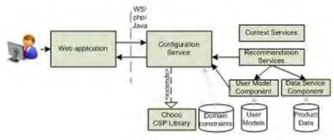
In a constraint-based recommender system the knowledge is formulated as a constraint satisfaction problem (CSP) in which some constraints are given explicitly by the user (e.g., an apartment buyer may state that he or she is interested in two bedroom apartments) or implicitly from the knowledgebase (a family with one child need an apartment with at least two bedrooms). An approach for implementing a constraint-based recommender system has been outlined in (Zanker, Aschinger, & Jessenitschnig, 2010). The structure of the proposed system is shown in Figure 2-3.

15

Figure 2-3. An architecture of constraint-based recommender systems (Zanker, Aschinger, & Jessenitschnig, 2010)

As depicted in the figure, the architecture consists of a configuration service set, a CSP library and several recommender service instances which provide personalized instance rankings for a class of products. A service-oriented architecture supports communication via Web services (WS). In addition, it makes the system extensible to ensure that it can include additional recommendation services.

A constraint-based recommender system is typically defined by two sets of variables (VC, VPROD)

and three different sets of constraints (CR, CF, CPROD) which will be explained in the below

(Felfernig & Burke, 2008).

- VC variables show the possible requirements of customers (e.g., the customer needs a two

bedroom apartment).

- VPROD variables describe the properties of a given product (e.g., the number of bedrooms

for an apartment).

- CR constraints restrict the possible instantiations of customer properties.

- CF constraints define the relationship between customer’s requirements and a given

product.

- CPROD is defined in disjunctive normal form to impose restrictions on the possible

instantiations of variables in VPROD.

These variables and constraints are the main components of a constraint satisfaction problem. A solution for a constraint satisfaction problem is a set of values for variables which satisfy all constraints.

2.5.2

Case-based Recommender Systems

Case-based recommender systems use case-based reasoning (CBR) to generate recommendation. CBR is a problem solving methodology that handles a new problem by taking two major steps: first an already solved similar case is retrieved, then that case is reused to solve the current problem.

In case-based recommender systems the users partially describe their needs. In such systems the products to be recommended are modelled by the case base and a set of recommended products is retrieved from the case base by finding the products which are similar to the one partially described by the user. In these systems a product and a case are essentially considered as

16

identical objects. The problem component of the case is represented by a set of user requirements and a set of product features, and the product is the solution component of the case.

2.6

Demographic Recommender System

Demographic recommender systems use demographic information of users to find similar users. Then, a list of items that have good feedback from similar users are recommended to the target user. This approach is shown in Figure 2-4.

Figure 2-4. Demographic-based approach (Safoury & Salah, 2013)

2.7

Hybrid Recommender Systems

Each of the aforementioned recommender systems has its own advantages and disadvantages. Hybrid recommender systems take advantages of various techniques at the same time (Bobadilla, Ortega, Hernando, & Gutiérrez, 2013). For example, collaborative filtering techniques ignore items’ properties and just focus on users’ similarities. Thus, combining collaborative filtering and content based methods will consider both users and items and may result in a more accurate recommendation. There are four main approaches for combining collaborative filtering with content-based filtering into a hybrid recommender system as follows (Mortensen, 2007):

- Combining separate recommender systems: Individual systems are implemented and the

final predication is calculated from the individual system predictions.

- Adding content-based characteristics to the collaborative filtering: In this approach,

content-based techniques are used when calculating the similarity between two users.

- Adding collaborative characteristics to the content-based approach: This approach uses

CF techniques when constructing user profile.

- Developing a single unifying recommendation approach: This approach unifies CF with

content-based into one general model.

It is also possible to combine CF with other approaches for example with demographic or knowledge based approaches.

17

2.8

Context-aware Recommender Systems

With the evolution of the web, mobile computing and wireless sensor networks (WSN), recommender systems tend to use contextual information (i.e., implicit information) as time, location, and sensed data along with the other type of data (i.e., explicit information) traditionally used for recommender systems. Gathering this kind of information can be applied to other user’s activities: ordering food, using public transport, visiting websites, etc.

An application of using context information is e-commerce personalization. For instance, supermarkets are interested in advertising new items and deals to their potential customers who are usually the people that live nearby.

In (Mayuri & Rajesh, 2013) a recommender system for both taxi drivers and taxi passengers has been proposed which uses GPS trajectories of taxicabs. The system infers the information about the routes, passengers’ mobility patterns, and taxi drivers’ picking-up/dropping-off behaviours. On the one hand, the system recommends taxi drivers the routes in which more passengers are likely to be waiting for taxi, and on the other hand, the system recommends passengers the routes that they can easily find vacant taxis.

There are two major concerns with using implicit information in recommender systems. First, there are some concerns about privacy preservation (Bilge & Polat, 2012). Second, since recommender systems are often used in ecommerce, some producers may cheat and state that their products have been recommended more than their competitors (Bobadilla, Ortega, Hernando, & Gutiérrez, 2013).

2.9

Cross-Domain Recommender Systems

Majority of recommender systems have been designed for a single domain. In (Fern´andez-Tob´ıas, Cantador, Kaminskas, & Retrieval., 2012) a domain is defined as “a set of items that share certain characteristics that are exploited by a particular recommender system”. These characteristics are users’ ratings and items’ attributes.

As already mentioned, single domain recommender systems often suffer from data sparsity and cold start problems. One solution for these problems could be considering data from different domains. This type of recommender systems are called cross-domain recommender systems. For example, a cross-domain recommender system may recommend movies, books, and music, at the same time. A person who likes romantic movies may also like a romantic book.

Cross-domain recommender systems are mainly classified based on domain levels as follows (Cantador & Cremonesi, 2014):

- Attribute level - items can be assigned to different domains based on their descriptions.

For example, one may consist of pop audio recordings, while another may contain jazz music.

- Type level - items with different types may share common attributes. For example,

although movies and books have different types, they have common genres, such as comedy, drama, and horror.

- Item level - items from different domains may have different types and attributes. For

18

- System level - items which belong to different recommender systems may have the same

type and may share many common attributes. For example, movies from MovieLens and the Internet Movie Database (IMDb) may belong to different domains.

2.10

Bio-inspired Approaches

Bio-inspired algorithms have been used in implementation of recommender systems. In this section, I review some of these approaches which are close to my research.

2.10.1

Genetic Algorithm

In (Bobadilla, F. Ortega, Hernando, & J. Alcalá, 2011), genetic algorithm (GA) has been used to calculate the similarity between users. Assuming users rate the items in the range [m,M] (e.g., for Movielens the rating range is [1,5]), each user’s rating is represented by a vector rx=(rx(1),rx(2),…,rx(I)) where I is the number of items and rx(i) is the user’s rating for item i. rx(i) = 

means that the user has not rated item i yet. Here are two examples of item vectors for two users: r1= (4,5, ,3,2, ,1,1,4)

r2= (4,3,1,2, ,3,4, ,2)

Then, for each pair of users x and y another vector is calculated: vxy=(vxy(0),…,vxy(M-m)) where vx,y(i)

represents the number of items rated by both users x and y with an absolute difference of i divided by the total number of items rated by both users. For example, v1,2 for the above users is as

follows:

v1,2=(1/5,1/5,2/5,1/5,0)

Then, the similarity function is calculated from the following formula:

𝑠𝑖𝑚

(𝑥, 𝑦) =

∑

𝑤

𝑥

𝑖=0

(2-19)

Where w=(w(0)_,…,w(M-m)_{) is a weighting vector whose elements lie in the range [-1,1]. The optimal}

value of w is calculated using GA. The proposed GA algorithm consists of the following steps:

- Initial population: Chromosomes are random values for w.

- Fitness function: The fitness function is the mean absolute error (MAE) of the

recommender system and is calculated using the following formula:

𝑓𝑖𝑡𝑛𝑒𝑠𝑠 = 𝑀𝐴𝐸 =

∑

#𝐼𝑢

𝑢𝑈

(2-20)

Where #U represents the number of users and #Iu represents the number of items rated

by user u. Pui uses the following equation to calculate the prediction of user u to item i:

𝑝

= 𝑟

̅ +

(2-21)

Where 𝑟̅ _𝑢represents the mean of user u ratings.

- Selection: Individuals are selected based on their fitness values.

- Crossover: One-point crossover has been used with a probability of 0.8. - Mutation: A single point mutation with a probability of 0.02 has been used.

19

The algorithm continues until an individual with a fitness value lower than a threshold (0.78 for Movielens) is found.

2.10.2

Ant Colony

The system presented in (P. Bedi & Kaur, 2009) consists of two phases: 1- Offline phase (data pre-processing)

In the first phase, ant colony (ACO) metaheuristic is used for clustering the users. This phase consists of four steps as follows:

Step 1: The user-item matrix is normalized.

Step 2: Users are clustered using ant based clustering technique. For N users and K clusters, a solution string is a vector with N elements each of which is a number in the range [1,k] which shows the cluster of the corresponding user. An example of a solution string for 10 users and 3 clusters is as below:

2 3 3 2 1 1 2 2 3 1

Which shows that the first user belongs to cluster 2, the second user belongs to cluster 3, etc. In each iteration, the algorithm executes three steps:

- Agents (ants) generate a pool of solutions using the modified pheromone trail from the

previous iteration

- Local search operation is performed on the newly generated solutions - The pheromone matrix trail gets updated

The algorithm continues until one solution with a fitness function lower than a threshold is found.

Step 3: The cluster-head of each cluster is determined. The user with minimum Euclidian distance to other users in the cluster is selected as the cluster-head.

Step 4: The initial pheromone of each cluster is calculated using the following formula:

𝑝ℎ𝑒𝑟

(𝑡) =

(2-22)

2- Online phase (recommendation for the active user) This phase consists of six steps as follows:

Step 1: The probability of the active user’s membership to each cluster is calculated to determine which cluster is more likely to accommodate the active user. The probability of choosing cluster i for the active user is calculated using the following formula:

𝑃

(𝑡) =

𝑗(𝑡)×𝑠𝑖𝑚𝑗 𝐾

20

Where pheri(t) is the amount of pheromone of cluster i at time t, simi is the similarity of the

active user and the head-cluster of cluster i, and K is the total number of clusters.

Step 2: The quality of ratings for each item in a cluster is calculated using the following formula:

𝑄 =

√𝑣𝑎𝑟

(2-24)

Where UB is the upper bound of ratings, avg_rating is the average of ratings, and var is the variance of ratings for the item in the chosen cluster. The higher value of Q means the quality of ratings for this item in the given cluster is better (i.e., users in this cluster have rated this item similarly).

Step 3: After calculating the quality of ratings for a given item in clusters, those clusters whose Q value differs at most 0.1 with the highest Q are chosen for predicting the active user’s rating for that item. The predicted rating is calculated from the following formula:

𝑅𝑎𝑡𝑖𝑛𝑔 =

∑𝑛𝑜_𝑐𝑐𝑐𝑐=1 𝑄𝑐𝑐 (2-25)

Where no_cc is the number of clusters, Qcc is the quality of cluster cc, and avg_rating is the average of ratings for the item in the chosen cluster.

Step 4: The pheromone associated with each cluster i is updated using the following formula:

𝑝ℎ𝑒𝑟

(𝑡) = (1 − 𝜌) × 𝑝ℎ𝑒𝑟

(𝑡 − 1) + ∇𝑄 × 𝑝ℎ𝑒𝑟

(𝑡 − 1)

Where  is the pheromone evaporation rate, Qcc is the quality of cluster cc, and no_cc is the number of clusters.

Step 5: The top N recommendations are provided to the active user.

Step 6: The pheromone information is stored for the future recommendations.

2.11

Summary

In this chapter, the concepts of recommender systems have been explained and past research on recommender systems which are more related to the present research have been reviewed. One of the most popular approaches in developing recommender systems is collaborative filtering (CF) which relies on the similarity of users. However, CF suffers from several problems: cold-start, sparsity, and scalability.

21

One technique which can solve the scalability problem is clustering the users. Users who are more similar to each other are grouped in one cluster. To recommend an item to the active user, his/her cluster must be determined first and then, based on the ratings of the users in the cluster, the rating of the active user for this item is calculated.

One of the major concerns with existing clustering techniques is the accuracy. Bio-inspired optimization techniques can help to improve the accuracy of the clustering algorithms.

Hence, this research proposes a new clustering approach which uses genetic algorithm (GA) for improving the quality of clusters. GA is one of the most popular and most effective metaheuristics whose convergence is often faster than other metaheuristics.

Another problem with existing CF techniques which will be also addressed in this thesis is considering the time factor when building clusters. This comes from the fact that the similarity of users may change over time. So, recent interactions of users receive higher priority when they are clustered.

22

23

This chapter proposes the cluster-based collaborative filtering method which consists of two phases: offline and online. In the offline phase, users are clustered. In the online phase, the appropriate cluster or clusters are selected for the target user and his/her ratings for unrated items are calculated based on the ratings of his/her cluster members. The proposed method is called CFGA.

3.1

Offline Phase

For clustering the users genetic algorithm (GA) is used which consists of the following steps (Ghosh, Biswas, Sarkar, & Sarkar, 2010):

 Initial population

The initial population in genetic algorithm is a set of proposed solutions to the problem which are called chromosomes.

 Chromosomes

Each chromosome is a proposed solution to the problem. In clustering, the length of chromosomes is the number of users and each gene from each chromosome represents the cluster of the corresponding user. In fact, the format of the chromosome in the proposed method for N users will be as follows:

Cluster Number of User

1 Cluster Number of User 2 Cluster Number of User 3 ... Cluster Number of User N

For example, if we have 10 users and 3 clusters, a sample chromosome can be as follows:

2 1 3 2 3 1 2 3 1 2

 Generating initial population

The initial population is generated based on the user estimation of the number of clusters. Then, chromosomes are generated randomly. In fact, if we have N users and K clusters, chromosomes are vectors of length N whose elements are random numbers in the range [1, K].

 Cluster-heads

In the proposed method, cluster-heads are users who have sufficient interaction with the system and are scattered sufficiently in the user space to have a perfect coverage of the user space. Selecting cluster-heads appropriately will have a significant impact on the quality of the clusters. Cluster-heads must.

In this method, first, the mean of ratings and the number of transactions of each user are calculated. Users who have the most interactions with the system can be suitable cluster-heads if they can cover rate differences in the system and be scattered enough in the user space. For this purpose, I divide the user space into intervals of equal length. The number of intervals is the same as the number of clusters. In fact, if the number of clusters determined by the user is K, the length of each interval can be achieved by equation (3-1) where m̅ is the lowest mean of ratings, M̅ _{is the}

24

highest mean of ratings, K is the number of clusters proposed by the user, and L is the length of intervals.

𝑳 = 𝑴̅ −𝒎_𝑲̅

(3-1)

First, I identify the user who has the highest number of interactions with the system and consider him or her as the cluster-head of the interval in which he or she is located. Then, in the other intervals, I determine ⌈√Ni⌉ number of users who have had the highest number of interactions

with the system and select them as candidates for being cluster-heads. There are 𝑁𝑖 users in the ith _{interval. In the next step, I calculate the Euclidean distance between the candidates of each}

interval with the cluster-head of cluster 1 according to equation (3-2). In each interval, the user who has the longest distance with the first cluster-head is selected as the cluster-head. In (3-2), i is a user whose distance is calculated from cluster-head 1, j is the number of items rated by both users i and 1, n is the total number of items rated by both users and r(i,j) indicates the rates assigned to item j by user i.

𝑑𝑖𝑠𝑡𝑎𝑛𝑐𝑒(𝑖, 1) = √∑𝑛 (𝑟(𝑖, 𝑗) − 𝑟(1, 𝑗))2

𝑗=1

(3-2)

If there is no user in an interval, we can allocate users in a fewer number of clusters, thus I reduce the number of clusters.

 Fitness function

We consider a vector for each user X as the following:

rx = (rx1_{, rx}2_{, … , rx}n₎

where rxi _{denotes the rating given by user x to item i. For two users x and y, the absolute}

difference of ratings on each item is a number in the range [0,M-m] where M is the maximum rating and m is the minimum rating. A vector V can be formed where Vxy denotes the difference between ratings of vectors belong to users x and y. Length of the vector V equals M-m. Vxy(i) denotes the number of corresponding ratings with difference amount of i in both users’ rating vectors. V is normalized.

Vxy= (Vxy(0),Vxy(1),…Vxy(M-m) )

Then, the time difference vector of corresponding ratings in both users’ vectors is formed. If two users give rates r1 and r2 in times t1 and t2 to the same item, then the time difference is

calculated using equation

(3-3).

∆𝑇 = |𝑡2 − 𝑡1|

(3-3)

25 ∆𝑇𝑥𝑦 = (∆𝑇𝑥𝑦(0), ∆𝑇𝑥𝑦(1),… ∆𝑇𝑥𝑦(M-m))

For each gene of the produced chromosome, vectors V and ΔT are constructed to know its difference with the cluster-head. Then, the Quality vector is formed in which each element

Quality(i) for user X and cluster-head C is obtained from equation (3-4). Vxc(i) is the ith _element

of vector V and ∆Txc(i) is the ith _{element of vector ∆𝑇.}

𝑄𝑢𝑎𝑙𝑖𝑡𝑦(𝑖) = 𝑉 𝑥𝑐(𝑖) ∗_{1+∆𝑇𝑥𝑐(𝑖)}1

(3-4) Quality vector is formed as follows.

𝑄𝑢𝑎𝑙𝑖𝑡𝑦 = (𝑄𝑢𝑎𝑙𝑖𝑡𝑦(1), 𝑄𝑢𝑎𝑙𝑖𝑡𝑦(2), … . 𝑄𝑢𝑎𝑙𝑖𝑡𝑦((𝑀 − 𝑚) + 1)

(3-5)

M − m and M-m₂ have been considered as coefficients to maximize the impact of the important

elements of the Quality vector. Assuming that M = 5 and m = 1, the Quality factor is calculated using equation (3-6).

𝑄𝑢𝑎𝑙𝑖𝑡𝑦𝑥𝑦=

4∗𝑄𝑢𝑎𝑙𝑖𝑡𝑦(1)+2∗𝑄𝑢𝑎𝑙𝑖𝑡𝑦(2)+𝑄𝑢𝑎𝑙𝑖𝑡𝑦₍₃₎ 1 + ( 2∗𝑄𝑢𝑎𝑙𝑖𝑡𝑦₍₄₎+4∗𝑄𝑢𝑎𝑙𝑖𝑡𝑦₍₅₎)

(3-6) For each chromosome, the fitness function is calculated using equation (3-7) where fitness(i) is the fitness of chromosome i, N is the total number of users, and Quality_(j,c(j)) is the Quality vector for user j relative to its cluster-head 𝑐(𝑗).

𝑓𝑖𝑡𝑛𝑒𝑠𝑠(𝑖) = ∑𝑁𝑗=1𝑄𝑢𝑎𝑙𝑖𝑡𝑦(𝑗,𝑐(𝑗))

(3-7)  Selection

Chromosomes are selected for crossover using roulette wheel. In the first step, a probability is assigned to each chromosome which shows its chance to be selected for transfer to the genetic pool. In the second step, a rank is assigned to each chromosome based on its fitness value. The best chromosome is in rank 1 and the worst chromosome is in rank N where N represents the size of the current population (number of users). In the proposed method, the probability of each chromosome is obtained from equation (3-8) where p(i) is the probability of selecting chromosome i and N is the total number of chromosomes.

𝑝(𝑖) =𝑁(𝑁+1)𝑁−𝑖+1

2

26

After obtaining p(i) for each chromosome, its cumulative probability, q(i), is obtained using equation (3-9):

𝑞(𝑖) = 𝑝(𝑖) + 𝑞(𝑖 − 1)

(3-9) Then, a random number in the range [0, 1] is generated and the chromosome with the least cumulative probability greater than the random number will be selected.

 Crossover

Chromosomes that were transferred to the genetic pool in the selection process, are combined together. In the proposed algorithm a two-point merging is used in which two different points of chromosomes are selected randomly and the genes between these two points of the two chromosomes are displaced.

 Mutation

To avoid local minima, GA uses mutation. A random mutation is used in which a random number in the interval [1, N] is generated and the corresponding gene is replaced with a random number in the interval [1, K] where N is the total number of users and K is the number of clusters. After mutation, GA restarts with a new population and continues until the difference of the fitness of the current and previous chromosome becomes lower than a specific threshold. Then, the offline phase is finished and the last chromosome shows the cluster of each user.

3.2

Online phase

In this phase, the membership probability of the target user to each cluster is calculated to find his or her cluster. Then, the target user’s rating for each item is predicted based on his or her neighbouring users’ rating for that item as detailed in the following.

 Cluster Selection

First, the density of each cluster is calculated. The density of cluster i is shown by 𝜌_𝑖 and is obtained from equation (3-10):

𝜌𝑖=𝑛𝑢𝑚𝑏𝑒𝑟 𝑜𝑓 𝑢𝑠𝑒𝑟𝑠 𝑖𝑛 𝑐𝑙𝑢𝑠𝑡𝑒𝑟 𝑖_{𝑡𝑜𝑡𝑎𝑙 𝑛𝑢𝑚𝑏𝑒𝑟 𝑜𝑓 𝑢𝑠𝑒𝑟𝑠} (3-10)

In the next step, the Quality vector for the target user relative to the centre of each cluster is obtained from equation (3-11) where X is the target user and C(i) is the centre of cluster i.

|𝑄𝑢𝑎𝑙𝑖𝑡𝑦𝑥,𝑐(𝑖)| =

4∗𝑄𝑢𝑎𝑙𝑖𝑡𝑦_{𝑥,𝑐(𝑖)(1)}+2∗𝑄𝑢𝑎𝑙𝑖𝑡𝑦_{𝑥,𝑐(𝑖)(2)}+𝑄𝑢𝑎𝑙𝑖𝑡𝑦_{𝑥,𝑐(𝑖)(3)}

1 + ( 2∗𝑄𝑢𝑎𝑙𝑖𝑡𝑦_{𝑥,𝑐(𝑖)(4)}+4∗𝑄𝑢𝑎𝑙𝑖𝑡𝑦_{𝑥,𝑐(𝑖)(5)}) (3-11)

Then, the probability of cluster i to be selected for the target user is obtained from (3-12) where Pi is the probability of selecting cluster i, ρ_i is the density of cluster i, and k is the total

number of clusters.

𝑃𝑖 = 𝜌𝑖∗|𝑄𝑢𝑎𝑙𝑖𝑡𝑦 (𝑥,𝑐(𝑖))|

∑𝑘 𝜌_𝑖∗|𝑄𝑢𝑎𝑙𝑖𝑡𝑦(𝑥,(𝑐𝑖))|

27

Clusters whose probabilities lie in the following intervals will be selected: The highest probability obtained ≥ Pi ≥ the highest probability obtained – α

Where α is a parameter that adjusts the number of selected clusters. In fact, it is likely that the target user belongs to more than one cluster.

 Prediction of Rating

Among selected clusters for the target user, clusters with higher credibility are considered for predicting his or her ratings. Creditability of users’ ratings in a cluster is high if cluster members have similar ratings. To realize the extent of closeness of users’ ratings in a cluster, standard deviation of ratings is used by which a factor called rating similarity in cluster i is calculated by equation (3-13). max_ 𝑟𝑎𝑡𝑒 is the upper limit of rating in cluster i, R̅_{(i) is the mean of ratings}

in cluster i, and 𝛿(𝑖) is the standard deviation of ratings in cluster i.

𝑠𝑖𝑚𝑖𝑙𝑎𝑟𝑖𝑡𝑦 𝑜𝑓 𝑟𝑎𝑡𝑖𝑛𝑔 𝑖𝑛 𝑐𝑙𝑢𝑠𝑡𝑒𝑟(𝑖) = (max_ 𝑟𝑎𝑡𝑒 + 𝑅̅(𝑖))

2 ∗ max_ 𝑟𝑎𝑡𝑒 + 𝛿(𝑖)

(3-13) Clusters which satisfy the following condition will be selected:

The highest similarity obtained ≥ the similarity obtained ≥ the highest similarity obtained – _β Where β is a parameter to adjust the number of selected clusters.

Finally, the predicted rating for item i is obtained from equation (3-14) where cs is the number of selected clusters for the target user, similarity( j) is the amount of similarity of ratings in cluster j, R̅_{(j) is the mean of ratings for item i in cluster j, and R(i) is the predicted rate of the}

target user to item i.

𝑅(𝑖) = ∑𝑐𝑠𝑗=1𝑠𝑖𝑚𝑖𝑙𝑎𝑟𝑖𝑡𝑦( 𝑗)∗𝑅̅(𝑗)

∑𝑐𝑠_𝑗=1𝑠𝑖𝑚𝑖𝑙𝑎𝑟𝑖𝑡𝑦(𝑗)

(3-14)

3.3

Evaluation

The CFGA method has been implemented in C#on a PC running Windows 10. In this section, it is evaluated and the quality of its recommendations is compared with similar methods.

3.3.1

Datasets

Two datasets from Movielens have been used to evaluate the proposed method. The characteristics of the datasets are detailed in Table 3-1.

Table 3-1. The Movielens datasets used for evaluation

Data set (1)

Data set (2)

28

Number of movies

983

3900

Number of ratings

100000

1000209

3.3.2

Evaluation Metrics

To evaluate the proposed method, I use Mean Absolute Error (MAE) and Accuracy metrics have been used. MAE is a statistical metric which is actually calculated by the numerical difference between the predicted rate and the actual rate as shown in equation Error! Reference source not found. where Pi,j is the predicted rate, ri,j is the actual rate of user i to item j and n is the total

number of recommendations in the system. Lower MAE means higher precision of the method (Gunawardana & Shani, 2009).

𝑴𝑨𝑬 =∑ 𝑷𝒊,𝒋 𝒊,𝒋 − 𝒓𝒊,𝒋

𝒏

(3-15)

Accuracy metric evaluates the effectiveness of a collaborative filtering algorithm in helping users to select high-quality items. This metric is based on the assumption that the process of prediction is a binary process which means either an item is of the user’s interest, in this case it is called a positive item, or it is not of the user’s interest, which it is called a negative item. For this evaluation, the following four factors must be measured (Tan, Steinbach, & Kumar, 2005):

 True-Positive (TP): which is the number of positive items that have been predicted as positive.

 False-Positive (FP): which is the number of negative items that have been predicted as positive.

 False-Negative (FN): which is the number of positive items that have been predicted as negative.

 True-Negative (TN): which is the number of negative items that have been predicted as negative.

Accuracy of the method is calculated by the following equation: Accuracy =_{(TP+FN+𝐹𝑃+𝑇𝑁)}𝑇𝑃+𝑇𝑁

(3-16)

3.3.3

Parameters of the Genetic Algorithm

The initial population size of GA in CFGA is 100. The crossover and mutation rates have been

considered as 0.6. At first, users are clustered in the offline phase using the training dataset

and, in the online phase, the test dataset is used for evaluation. 80% of the data has been

considered randomly for training and 20% for testing phase

3.3.4

Results

As it is shown in

, when the number of users is small, the error of CFGA is high and

the system is not stable. When the number of users increases, the number of recommendations

29

in the system is also increased. In this case, the performance of the method is improved. The

error of the method is 77% for 943 users.

Figure 3-1

.

MAE of the CFGA method (dataset 1)

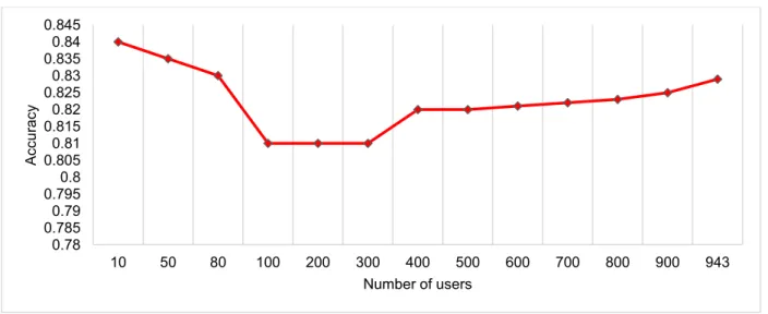
Figure 3-2

depicts the accuracy of the CFGA method. Similarly to MAE, when the number of

users is small, the quality of clusters is not satisfactory. As a result, when the system predicts

user ratings in the online phase, the accuracy is low. While the number of users increase, better

clusters are formed and prediction of ratings become more accurate. The accuracy of CFGA is

82.9% for 943 users.

Figure 3-2.

Accuracy of the CFGA method (dataset 1)

0.65 0.67 0.69 0.71 0.73 0.75 0.77 0.79 0.81 0.83 0.85 0.87 0.89 10 50 80 100 200 300 400 500 600 700 800 900 943 M AE Number of users 0.78 0.7850.79 0.7950.8 0.8050.81 0.8150.82 0.8250.83 0.8350.84 0.845 10 50 80 100 200 300 400 500 600 700 800 900 943 Ac cu ra cy Number of users

30

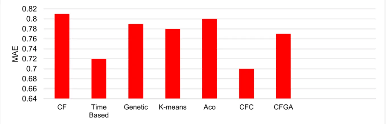
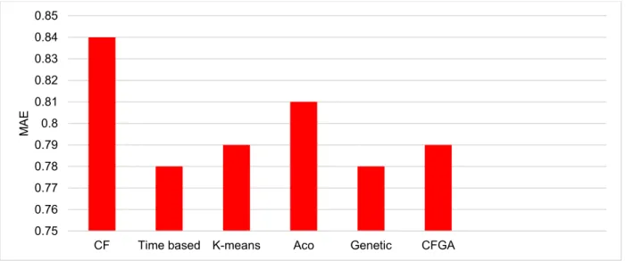
In the next step, the error of CFGA is compared with the error of previous research. CF uses

the traditional method of collaborative filtering in which Pearson similarity factor is used to

find user’s neighbours. Time-based method (Rafeh & Bahremand, 2012) is a collaborative

filtering method that incorporates the time factor in the similarity function. Genetic is also a

collaborative filtering method that uses genetic algorithm to calculate the similarity between

users (Bobadilla, Ortega, Hernando, & Gutiérrez, 2013). CFC method combines collaborative

filtering method and constraints. ACO uses ant colony algorithm to determine the similarity of

users (Bedi, Sharma, & Kaur, 2009). K-means (Dakhel & Mahdavi, 2013) uses the K-means

clustering algorithm for recommender systems.

Figure 3-3

and

compare the error and accuracy of CFGA with the previous methods.

As can be seen in the figures, the quality of CFGA is better than the traditional CF, ACO,

genetic and K-means methods. However, the Time-based and CFC methods outperform

CFGA.

Figure 3-3.

Comparison of CFGA and the previous methods in terms of MAE (dataset 1)

Figure 3-4.

Comparison of CFGA and the previous methods in terms of Accuracy (dataset 1)

0.64 0.66 0.680.7 0.72 0.74 0.76 0.780.8 0.82 CF Time

Based Genetic K-means Aco CFC CFGA

M AE 0.81 0.815 0.82 0.825 0.83 0.835 0.84 0.845

CF Time based Aco CFC CFGA

Ac

cu

ra

31

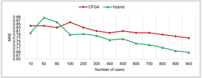
As a second test, I used dataset 2 which includes 6040 users who have done a million rates in

the system. 80% of the data has been considered randomly for training and 20% for testing

phase. Due to its larger volume, this dataset is more appropriate for evaluating the performance

of recommender systems than the first dataset. CFGA has been tested on this dataset and the

factors of MAE and accuracy have been compared for CFGA and previous researches that have

been evaluated using this dataset

. As depicted in

, MAE of CFGA is 79% which is

lower than CF, K-means, and ACO, but higher than Time-based and Genetics.

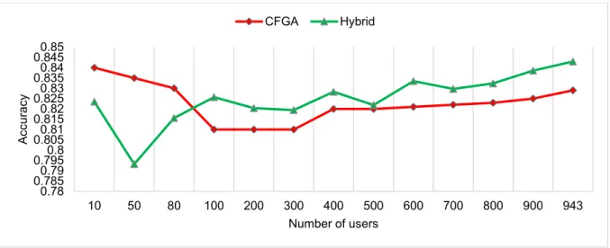
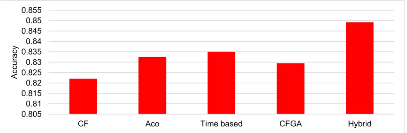
compares the performance of the methods in terms of Accuracy which is %82.9 for the

proposed method. This is higher than CF and lower than Time-based and ACO.

Figure 3-5.

Comparison of CFGA and the previous methods in terms of MAE (dataset 2)

Figure 3-6.

Comparison of CFGA and the previous methods in terms of Accuracy (dataset 2)

1 _{Some of the previous researches did not use this dataset for evaluation and hence are not compared with the first method.}

0.75 0.76 0.77 0.78 0.79 0.8 0.81 0.82 0.83 0.84 0.85

CF Time based K-means Aco Genetic CFGA

M AE 0.815 0.82 0.825 0.83 0.835 0.84

CF Aco Time based CFGA

Ac

cu

ra

32

As can be seen from the results, compared to other approaches, the CFGA method is better

than traditional collaborating filtering (CF) and K-means. However, Time-based approach and

CFC outperform CFGA. This was my motivation to modify CFGA and to propose a hybrid

method in the hope of improving its performance. The hybrid method will be discussed in the

next chapter.

3.4

Summary

In this chapter proposes a cluster-based recommendation method, CFGA, which consists of

two stages: offline and online. In the offline phase, users are clustered based on their

similarities. In the online phase, the targets user’s ratings are predicted for items not previously

rated by this user.

In the CFGA method, genetic algorithm (GA) is used for clustering. For the fitness function,

CFGA focuses on the difference of ratings and the time of ratings for users when clustering

them.

Compared to other approaches, CFGA is better than traditional collaborating filtering (CF) and

K-means. However, Time-based approach and CFC outperform CFGA. Another problem with

CFGA is the cold start problem which is a common issue with collaborative filtering methods.

The next chapter proposes the hybrid approach which improves CFGA by considering several

other factors in the fitness function: user’s age, gender, and occupation.

33

34

As it was discussed in the previous chapter, after evaluating the CFGA method in terms of error and accuracy of the prediction using two datasets from Movielens, I found that when the number of users grows, the performance of the method is increased because of creating high quality clusters. Compared to other approaches, CFGA is better than existing research. However, there are some approaches that outperform CFGA. Thus, I modified CFGA in a hope of improving its performance. The second proposed method is a hybrid approach which, in addition to collaborative filtering and genetic algorithm, incorporates demographic information about users. Similarly to CFGA, the hybrid method consists of two phases: offline and