2010/59
!
Nonnegative factorization
and the maximum edge biclique problem
Nicolas Gillis and François Glineur
Center for Operations Research
and Econometrics
Voie du Roman Pays, 34
B-1348 Louvain-la-Neuve
Belgium
http://www.uclouvain.be/core
D I S C U S S I O N P A P E R
CORE DISCUSSION PAPER 2010/59
Nonnegative factorization and the maximum edge biclique problem Nicolas GILLIS 1 and François GLINEUR2
October 2010
Abstract
Nonnegative matrix factorization (NMF) is a data analysis technique based on the approximation of a nonnegative matrix with a product of two nonnegative factors, which allows compression and interpretation of nonnegative data.
In this paper, we study the case of rank-one factorization and show that when the matrix to be factored is not required to be nonnegative, the corresponding problem (R1NF) becomes NP-hard. This sheds new light on the complexity of NMF since any algorithm for fixed-rank NMF must be able to solve at least implicitly such rank-one subproblems.
Our proof relies on a reduction of the maximum edge biclique problem to R1NF. We also link stationary points of R1NF to feasible solutions of the biclique problem, which allows us to design a new type of biclique finding algorithm based on the application of a block-coordinate descent scheme to R1NF. We show that this algorithm, whose algorithmic complexity per iteration is proportional to the number of edges in the graph, is guaranteed to converge to a biclique and that it performs competitively with existing methods on random graphs and text mining datasets.
Keywords: nonnegative matrix factorization, rank-one factorization, maximum edge biclique problem, algorithmic complexity, biclique finding algorithm.
JEL Classification: 15A23, 68Q25, 90C06, 90C27 90C35, 90C59
1 Université catholique de Louvain, CORE, B-1348 Louvain-la-Neuve, Belgium. E-mail: [email protected]. 2 Université catholique de Louvain, CORE, B-1348 Louvain-la-Neuve, Belgium. E-mail: [email protected].
This author is also member of ECORE, the association between CORE and ECARES.
We thank Pr. Paul Van Dooren and Pr. Laurence Wolsey for helpful discussions and advice. The first author is a research fellow of the Fonds de la Recherche Scientifique (F.R.S.-FNRS).
This paper presents research results of the Belgian Program on Interuniversity Poles of Attraction initiated by the Belgian State, Prime Minister's Office, Science Policy Programming. The scientific responsibility is assumed by the authors.
1
Introduction
(Approximate) Nonnegative matrix factorization (NMF) is the problem of approximating a given nonnegative matrix by the product of two low-rank nonnegative matrices: given am×n nonnegative
real matrix M ∈ Rm+×n and a factorization rank r, one has to compute two nonnegative matrices V ≥0 andW ≥0 of dimensions m×rand r×nsuch that
M ≈V W . (1.1)
Typically the quality of the approximation is measured by the Frobenius norm1 of the residual error
matrix, and one tries to solve: min
V∈Rm×r,W∈Rr×n||M−V W|| 2
F such thatV ≥0, W ≥0. (NMF)
This problem was first introduced in 1994 by Paatero and Tapper [26], and more recently received a considerable interest after the publication of two papers by Lee and Seung [21, 22]. It is now well established that NMF is useful in the framework of compression and interpretation of nonnegative data ; it has for example been applied in analysis of image databases, text mining, interpretation of spectra, computational biology and many other applications (see [2, 8, 9] and references therein). Unfortunately (NMF) is a NP-hard optimization problem [29] and therefore we cannot expect to solve it up to global optimality in a reasonable computational time. Therefore most practical algorithms proposed to find approximate solutions of (NMF), based on iterative optimization schemes (see, e.g., [2, 3, 5, 6, 9, 14, 19, 23]), offer no guarantee on the global optimality of the solutions they provide. How can one interpret the outcome of a NMF? Assume each columnM:j of matrixM represents an
element of a data set: expression (1.1) can be equivalently written as
M:j ≈
�
k
V:kWkj, ∀j, (1.2)
where each element M:j is decomposed into a nonnegative linear combination (with weights Wkj)
of nonnegative basis elements ({V:k}, the columns of V). Nonnegativity of V allows interpretation
of the basis elements in the same way as the original nonnegative elements in M, which is crucial
in applications where the nonnegativity property is a requirement (e.g., where elements are images described by pixel intensities or texts represented by vectors of word counts). Moreover, nonnegativity of the weight matrix W corresponds to an essentially additive reconstruction which leads to a part-based representation: basis elements will represent similar parts of the columns of M. Sparsity is
another important consideration: finding sparse factors improves compression and leads to a better part-based representation of the data [18]. In particular, when dealing with sparse matrices, NMF can be interpreted as a biclustering model, see [10, 20] and references therein. In fact, each rank-one factor of the decomposition will correspond to a dense rectangular submatrix ofM (a bicluster),
enabling NMF to detect interactions between columns and rows of the matrixM (e.g., in text mining
applications, NMF extracts closely related sets of texts and words [11]).
In the special case where we seek a rank-one factorization (i.e. when r = 1), NMF is known
to be polynomially solvable (using the Eckart-Young and Perron-Frobenius Theorems, it reduces to computing the dominant left and right singular vectors). The central problem studied in this paper, called rank-one nonnegative factorization (R1NF), is an extension of rank-one NMF where the matrix to be approximated by the outer product of two nonnegative vectors is now allowed to contain negative elements.
R1NF is introduced in Section 2, where it is shown that allowing negative elements in the matrix transforms the polynomially solvable rank-one NMF problem into a NP-hard problem. The reduction
1||A||
used on the proof is based on the problem of finding a maximum edge biclique in a bipartite graph. Because any algorithm designed to solve NMF must at least implicitly solve R1NF problems, this hardness result sheds new light on the limitations of NMF algorithms and the complexity of NMF when the factorization rank ris fixed.
In Section 3, stationary points of the R1NF problem used in the above-mentioned reduction are shown to coincide with bicliques of the corresponding graph. Building on that fact, Section 4 introduces a new type of biclique finding algorithm that relies on the application of a simple nonlinear optimization scheme (block-coordinate descent) to the equivalent R1NF problem considered earlier, which only requires for each iteration a number of operations proportional to the number of edges of the graph. This method is then compared to a greedy heuristic and an existing algorithm [12] on some synthetic and text mining datasets, and is shown to perform competitively.
2
Rank-one Nonnegative Factorization
(R1NF)
2.1
Motivation
Solving (NMF) amounts to findingr nonnegative rank-one factors V:kWk:, each having to satisfy the
following equality as well as possible
V:kWk:≈M−
�
i�=k
V:kWk:=. Rk�0 ∀k,
i.e. each of them should be the best possible nonnegative rank-one approximation of the corresponding residual matrix, denotedRk. It is important to notice here that, unlike input matrixM, matricesRk
can contain negative elements. Therefore, any NMF algorithm has to solve, at least implicitly, the following subproblems min V:k∈Rm,W k:∈Rn ||M−V W||2 F =||Rk−V:kWk:||F2 such thatV:k≥0, Wk: ≥0, (2.1)
for each k. We may wonder whether theses subproblems can be solved efficiently, i.e., ask ourselves
Is it possible to compute efficiently the best rank-one nonnegative approximation of a ma-trix which is not necessarily nonnegative?
An interesting observation is that computing the globally2optimal value ofV
:k for a given value of
Wk: can be done in closed-form (and similarly for computing the optimal value ofWk: for a fixedV:k):
V:∗k = argminV:k≥0||Rk−V:kWk:|| 2 F = max � 0, RkW T k: ||Wk:||22 � , (2.2) Wk∗: = argminWk:≥0||Rk−V:kWk:|| 2 F = max � 0, V T :kRk ||V:k||22 � . (2.3)
One can therefore try to solve (2.1) and, more generally, (NMF) by updating successively the columns ofV and rows ofW. This scheme, which amounts to a block-coordinate descent method, was proposed
by Cichocki et al. [5] and called hierarchical alternating least squares (HALS) (see also [4, 17]). It has been observed to work remarkably well in practice, and in particular it clearly outperforms the standard multiplicative updates (MU) of Lee and Seung [22].
2.2
Definition of R1NF and Implications for NMF
In order to shed some light on the above question, we define the problem of rank-one nonnegative factorization3 (R1NF) to be the variant of rank-one NMF where the matrix to be factorized can be
any real matrix, i.e., is not necessarily nonnegative. Formally, given anm×n real matrixR∈Rm×n
+ ,
one has to find a nonnegative column vectorv∈Rm and a nonnegative row vectorw∈Rn such that
the nonnegative rank-one product4 vw is the best possible approximation (in the Frobenius norm) of
matrixR:
min
v∈Rm,w∈Rn||R−vw|| 2
F such that v≥0, w≥0. (R1NF)
The next subsection shows that, in contrast with standard rank-one NMF, this problem is NP-hard, which provides the following new insights about the NMF problem:
• We cannot expect to be able to solve subproblems (2.1) efficiently up to global optimality, and
the HALS algorithm most probably cannot be improved with a better scheme for successively computing rank-one factors V:kWk: arising in (2.1). More generally, any algorithm for NMF
cannot expect to solve at each iteration a subproblem where a given column of V:k and its
corresponding rowWk: are to be optimized simultaneously which shows that, in that sense, the
partition of variables for block-coordinate schemes such as alternative nonnegative least squares (ANLS, optimizing V andW alternatively) [20] and (implicitly) HALS is best possible.
• Recall that the NP-hardness result characterizing NMF requires both the dimensions of matrix
M and the factorization rankrofM increase, and that the complexity of NMF for a fixed rankr
is currently not known (except5in the polynomially solvable rank-one case). Our hardness result
on (R1NF) therefore suggests that NMF is also a difficult problem for any fixed rank r ≥ 2.
Indeed, even if one was given the optimal solution of a NMF problem except for a single rank-one factor, it is not guaranteed that one would be able to find this last factor in polynomial-time, since the corresponding residual matrix is not necessarily nonnegative.
2.3
Complexity of R1NF and the Maximum Edge Biclique Problem in Bipartite
Graphs
In this section, we show how the optimization version of the maximum edge biclique problem (MB) can be formulated as a specific rank-one nonnegative factorization problem (R1NF-MB). Since the decision version of (MB) is NP-complete [27], this implies that rank-one nonnegative factorization (R1NF) is in general NP-hard.
Abipartite graph Gbis a graph whose vertices can be divided into two disjoint setsV1 andV2such
that there is no edge between two vertices in the same set
Gb= (V, E) =
�
V1∪V2, E⊆(V1×V2)
� .
AbicliqueKbis a complete bipartite graph, i.e., a bipartite graph where all the vertices are connected
Kb= (V�, E�) =
�
V1�∪V2�, E�= (V1�×V2�)
� .
3This terminology has already been used for the problem of finding a symmetric nonnegative factorization, i.e., one
where V=W, but we assign it a different meaning in this paper.
4In the sequel, it is always assumed thatv andware respectively a column and a row vector, i.e. that the rank-one
matrixvwis equal to the outer product ofv andw.
5In fact, testing whether a nonnegative matrix admits a rank-two nonnegative factorization can also be done in
polynomial time [7], but, when the answer is negative, finding the best possible rank-two approximate nonnegative factorization has unknown complexity status.
The so-called maximum edge biclique problem in a bipartite graph Gb = (V, E) is the problem of
finding a biclique Kb = (V�, E�) in Gb (i.e., V� ⊆ V and E� ⊆ E) maximizing the number of edges.
The decision problem: Given B, doesGb contain a biclique with at leastB edges? has been shown to
be NP-complete [27], and the corresponding optimization problem is at least NP-hard.
LetMb∈ {0,1}m×nbe the biadjacency matrix of the unweighted bipartite graphGb= (V1∪V2, E)
with V1 = {s1, . . . sm} and V2 = {t1, . . . tn}, i.e., Mb(i, j) = 1 if and only if (si, tj) ∈ E. We denote
by|E| the cardinality ofE, i.e., the number of edges inGb; note that |E| =||Mb||2F. The set of zero
values will be denotedZ ={(i, j)|Mb(i, j) = 0}, and its cardinality|Z|, with |E|+|Z|=mn. With
this notation, the maximum biclique problem in Gb can be formulated as
min v,w ||Mb−vw|| 2 F viwj≤Mb(i, j), ∀i, j, (MB) v∈ {0,1}m, w∈ {0,1}n.
In fact, one can check easily that this objective is equivalent to maxv,w�ijviwj since Mb, v and w
are binary: instead of maximizing the number of edges inside the biclique, one minimizes the number of edges outside.
Feasible solutions of (MB) correspond to bicliques ofGb. We will be particularly interested inmaximal
bicliques, which are bicliques not contained in a larger biclique.
The corresponding rank-one nonnegative factorization problem is defined as min
v∈Rm,w∈Rn||Md−vw|| 2
F such that v≥0, w≥0 (R1NF-MB)
where Md is the matrixMb where the zero values have been replaced by −d, i.e.
Md= (1 +d)Mb−d1m×n, d >0, (2.4)
and 1m×n is the matrix of all ones with dimension m×n. Although (R1NF-MB) is a continuous
optimization problem, we are going to show that, for a sufficiently large value of d, any of its
opti-mal solutions has to coincide with a binary optimal solution of the corresponding (discrete) biclique problem (MB), which will then imply NP-hardness of (R1NF).
Intuitively, if a −d entry ofMd is approximated by a positive value, say p, the corresponding term
in the squared Frobenius norm of the error is d2+2pd+p2. As d increases, it becomes more and
more costly to approximate −d by a positive number and we will show that, for d is sufficiently
large, negatives values of Md have to be approximated by zeros. Since the remaining values (not
approximated by zeros) are all ones, the optimal rank-one solution will be binary.
From now on, we say that a solution (v, w) coincides with another solution (v�, w�) if and only if vw=v�w� (i.e., if and only if v�=λvand w� =λ−1w for someλ >0). We also letM
+= max(0, M), M− = max(0,−M), min(M) = mini,j(Mij) and ||M||2 be the standard matrix 2-norm of M, i.e.
||M||2= maxx∈Rn,||x||2=1||M x||2=σmax(M) whereσmax(M) is the maximum singular value of M.
Lemma 1. Any optimal rank-one approximation with respect to the Frobenius norm of a matrix M
for whichmin(M)≤ −||M+||F contains at least one nonpositive entry.
Proof. IfM =0, the result is trivial. If not, we have min(M)<0 since min(M)≤ −||M+||F. Suppose
now (v, w)>0 is a best rank-one approximation ofM. Therefore, since the negative values of M are
approximated by positive ones and sinceM has at least one negative entry, we have
By the Eckart-Young theorem, the optimal rank-one approximationvw must satisfy
||M −vw||2F =||M||2F−σmax(M)2=||M||2F− ||M||22.
Clearly,
||M||2F =||M+||2F +||M−||2F and ||M||22≥min(M)2
so that we can write
||M −vw||2F ≤ ||M+||2F+||M−||2F −min(M)2≤ ||M−||F
which is in contradiction with (2.5).
We will need to use the following well-known result concerning (unconstrained) low-rank approxi-mations (see, e.g., [17, p. 29]).
Lemma 2. The local minima of the best rank-one approximation problem with respect to the Frobenius norm are global minima.
We can now state the main result about the equivalence of (R1NF-MB) and (MB).
Theorem 1. For d ≥ �|E|, any optimal solution (v,w) of (R1NF-MB) coincides with an optimal
solution of (MB), i.e., vw is binary and vw≤Mb.
Proof. We focus on the entries of vw which are positive and define their support as K=�i∈ {1,2, . . . , m}���vi>0
�
and L=�j ∈ {1,2, . . . , n}���wj >0
�
. (2.6)
We also define v� = v(K), w� =w(L) and Md� = Md(K, L) to be the subvector and submatrix with
indexes inK,LandK×L. Since (v, w) is optimal forMd, (v�, w�) must be optimal forMd�. Suppose
there is a−d entry inMd�, then
min(Md�) =−d≤ −
�
|E|=−||(Md)+||F ≤ −||(Md�)+||F,
so that Lemma 1 holds for M�
d. Since (v�, w�) is positive (i.e., it is located inside the feasible domain)
and is an optimal solution of (R1NF-MB) for Md�, (v�, w�) is a local minimum of the unconstrained
problem, i.e., the problem of best rank-one approximation. By Lemma 2, this must be a global minimum. This is a contradiction with Lemma 1: (v�, w�) should contain at least one nonpositive
entry. Therefore Md� does not contain any −d entry, and we have Md� =1|K|×|L| which implies than
v�w� =Md� by optimality (it is the unique rank-one solution v�w� with objective value equals to zero)
and finally allows to conclude that vw is binary andvw ≤Mb.
We have just proven the following theorem:
Theorem 2. Rank-one nonnegative factorization (R1NF)is NP-hard.
3
Stationary Points of
(R1NF-MB)
We have shown that optimal solutions of (R1NF-MB) coincide with optimal solutions of (MB) ford≥
�
|E|, whose computation is NP-hard. In this section, we focus on stationary points of (R1NF-MB)
instead: we show how they are related to the feasible solutions of (MB). This result will be used in Section 4 to design a new type of biclique finding algorithm.
3.1
Definitions and Notations
The pair (v, w) is a stationary point for problem (R1NF-MB) if and only if it satisfies its first-order
optimality conditions, i.e. if and only if
v≥0, µ= (vw−Md)wT ≥0 and v◦µ=0, (3.1)
w≥0, λ=vT(vw−Md) ≥0 and w◦λ=0, (3.2)
where ◦ denotes the component-wise multiplication. Of course, we are only interested in nontrivial
solutions and, assuming thatv�=0andw�=0, one can check that conditions (3.1)-(3.2) are equivalent
to v= max�0,Mdw T ||w||2 2 � and w= max�0,v TM d ||v||2 2 � . (3.3)
We define three sets of rank-one matrices:
1. Given a positive real numberd,Sd is the set of nontrivial stationary points of (R1NF-MB), i.e.6
Sd={vw∈R0m×n |(v, w) satisfies (3.3)};
2. F is the set of feasible solutions of (MB), i.e.
F ={vw∈Rm×n
|(v, w) is a feasible for (MB)},
3. B is the set of maximal bicliques of (MB), i.e., vw∈B if and only if vw∈F andvw coincides
with a maximal biclique.
3.2
Stationarity of Maximal Bicliques
The next theorem states that, for d sufficiently large, the only nontrivial feasible solutions of (MB)
that are stationary points of (R1NF-MB) are the maximal bicliques.
Theorem 3. Ford >max(m, n)−1, F ∩Sd =B.
Proof. Let show that vw ∈B if and only if vw ∈F and vw ∈Sd. By definition,vw belongs toB if
and only if vw belongs toF and is maximal, i.e.,
(*) �i such thatvi= 0 andMd(i, j) = 1,∀j s.t. wj�= 0,
(**) �j such thatwj = 0 andMd(i, j) = 1,∀i s.t. vi�= 0.
Since vw is binary and v �= 0, the nonzero entries of w must be equal to each other. Noting L the
support ofw (see Equation (2.6)), we then have wj = ||w||1
|L| =C, ∀j∈L,
for some C ∈ R+, where||x||1 = �ni=1|xi| for x ∈ Rn. Moreover, d > max(m, n)−1 so that (*) is
equivalent to
�i such that vi= 0 and Md(i,:)wT >0
⇐⇒ vi= 0⇒Md(i,:)wT ≤0 and vi�= 0⇒vi= C1 = ||M||dw(i,||:)1||1 = Md(i,:)w T ||w||2 2 . 6R 0=R\{0}
These are exactly the stationarity conditions for v�=0, cf. (3.3). By symmetry, (**) is equivalent to
the stationarity conditions for w, so that we can conclude that vw ∈ B if and only if vw ∈ F and
vw∈Sd.
Theorem 3 implies that, for d sufficiently large, B ⊂ Sd. It would be interesting to have the
converse affirmation, i.e. to show that for d sufficiently large, any stationary point of (R1NF-MB)
corresponds to a maximal biclique of (MB). As we will see later, this property unfortunately does not hold. However, the following slightly weaker result can be proved: asdgoes to infinity, the points inSd
get closer and closer to feasible solutions of (MB), i.e. to bicliques of the graphGb. As a consequence,
rounding stationary points of (R1NF-MB) ford sufficiently large will generate bicliques ofGb.
3.3
Limit Points of
S
dLemma 3. The set Sd is bounded, i.e., ∀d >0, ∀vw∈Sd:
||vw||2 =||v||2||w||2≤
�
|E|. Proof. For anyvw∈Sd, we have by (3.3)
||v||2= � � � � � �max�0,Mdw T ||w||2 2 ������ � 2≤ ||max(0, Md)wT||2 ||w||2 2 ≤ ||max(0, Md)||F ||w||2 = � |E| ||w||2 .
Lemma 4. For vw∈Sd, if Md(i, j) =−d and if (vw)ij >0, then
0< vi < ||v||1 d+ 1 and 0< wj < ||w||1 d+ 1. Proof. By (3.3), we have 0< wj||v||22=vTMd(:, j)≤ ||v||1−(d+ 1)vi ⇒ 0< vi< ||v||1 d+ 1.
The corresponding result forw is obtained similarly.
Theorem 4. As d goes to infinity, stationary points of (R1NF-MB) get arbitrarily close to feasible solutions of (MB), i.e., ∀� >0,∃D s.t. ∀d > D: max vw∈Sd min vbwb∈F || vw−vbwb||F < �. (3.4)
Proof. Letvw ∈Sd. We can assume w.l.o.g. thatvw >0 ; otherwise, we consider the subproblem with
the vectors v(K) andv(L) whereK (resp.L) is the support ofv (resp.w) and the matrix M(K, L),
see Equation (2.6). In fact, it is clear that if (v(K), w(L)) is close to a feasible solution of (MB)
for Mb(K, L), then (v, w) is for Mb. We also assume w.l.o.g. that ||w||2 = 1; in fact, if vw ∈ Sd,
�
λv1λw�∈Sd,∀λ >0. Note that Lemma 3 implies ||v||2≤
� |E|. By (3.3), v=MdwT and w= vTM d ||v||2 2 . (3.5)
Therefore, (v/||v||2, w) > 0 is a pair of singular vectors of Md associated with the singular value
||v||2 >0. IfMd =1m×n, the only pair of positive singular vectors of Md is
�
1
√m1m,√1n1n
�
so that
vw=Mb coincides with a feasible solution of (MB).
Otherwise, when Md�=1m×n, we define
A=�i���Md(i, j) = 1,∀j
�
and B=�j ���Md(i, j) = 1,∀i
�
, (3.6)
and their complements ¯A={1,2, . . . , m}\A, ¯B={1,2, . . . , n}\B; hence,
Md(A,:) =1|A|×n and Md(:, B) =1m×|B|.
These two sets clearly define the biclique A×B in graph Gb, or, equivalently, a (binary) feasible
solution (¯vA,w¯B) for problem (MB), where ¯vA is equal to one for indices in Aand to zero otherwise
(similarly for ¯wB and B). We are now going to show that, for d sufficiently large, vw is arbitrarily
close to ¯vAw¯B, which will prove our claim.
Using Lemma 4 and the fact that||x||1≤√n||x||2,∀x∈Rn, we get 0< v( ¯A)< � m|E| d+ 1 1|A¯| and 0< w( ¯B)< √ n d+ 11|B¯|. (3.7)
Therefore, since||w||2= 1 and ||v||2≤
� |E|, we obtain ||v( ¯A)w−0||F =||v( ¯A)||2||w||2< 1 d+ 1 � m�|E|�, and (3.8) ||vw( ¯B)−0||F =||v||2||w( ¯B)||2< 1 d+ 1 � n�|E|�. (3.9)
It remains to show that v(A)w(B) coincides with a biclique of the (complete) graph generated by Mb(A, B) =1|A|×|B| sincev( ¯A)w and vw( ¯B) tend to zero as d goes to infinity.
Notingkw= ||||vv||||12
2 and using (3.5), we getw(B) =kw1|B|. Combining this with (3.7) gives
1− |B¯| √ n d+ 1<||w|| 2 2− ||w( ¯B)||22=||w(B)||22=|B|kw2 ≤ ||w||22= 1. (3.10)
Moreover, (3.5) impliesv(A) =1|A|×mwT =||w||11|A| so that
|B|kw≤v(A) = (||w(B)||1+||w( ¯B)||1)1|A|<|B|kw+|B¯|
√
n
d+ 1. (3.11)
Finally, multiplying (3.11) bykw, combining it with (3.10) and noting that, since ||w||2= 1, we have kw ≤1, we obtain � 1−|B¯| √ n d+ 1 � 1|A|×|B| < v(A)w(B)< � 1 +|B¯| √ n d+ 1 � 1|A|×|B|. (3.12)
We can conclude that, for d sufficiently large, vw is arbitrarily close to a feasible solution ¯vAw¯B of
3.4
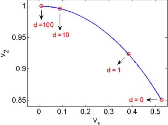
Example
Let Mb = � 0 1 1 1 � and Md= � −d 1 1 1 � . Clearly, � 0 1 0 1 �belongs to the set B, i.e., it corresponds to a maximal biclique of the graph generated by Mb. By Theorem 3, for d > 1, it belongs to Sd, i.e., [(1 1)T,(0 1)] is a stationary point of
(R1NF-MB).
For d >1, one can also check that the singular values ofMd are disjoint and that the second pair of
singular vectors is positive. Since it is a positive stationary point of the unconstrained problem, it is also a stationary point of (R1NF-MB). Asd goes to infinity, it must get closer to a biclique of (MB)
(Theorem 4). MoreoverMd is symmetric so that the right and left singular vectors are equal to each
other. Figure 1 shows the evolution7 with respect tod of this positive singular vector (v
1, v2), which
is such that (v1v2)T(v1v2) ∈ Sd. It converges to (0 1), which means that the outer product of the
left and right singular vectors converges to
� 0 0
0 1
�
, which is a biclique, i.e. a member of F. We
also note that this biclique is not maximal, which shows that the converse to Theorem 3 is false, even asymptotically asdgoes to infinity.
Figure 1: Evolution of (v1, v2).
Corollary 1. For
d≥2max(m, n)�|E|, (3.13) any stationary point vw ∈Sd of (R1NF-MB) can be rounded8 to generate a biclique of the graphGb
generated by Mb.
Proof. The condition
max vw∈Sd min vbwb∈F max ij (vw−vbwb)ij < 1 2,
is clearly sufficient to guarantee that rounding any stationary point of (R1NF-MB) will generate a biclique of Gb. Looking back at Theorem 4, one can check that this is satisfied (cf. Equations (3.8),
(3.9) and (3.12)) for d given by (3.13) (note that w.l.o.g. |E| ≥ max(m, n), i.e., that each row and
each column ofMb has at least one nonzero entry, otherwise they can be removed).
7By Wedin’s theorem (cf. matrix perturbation theory [28]), singular subspaces of Md associated with a positive
singular value are continuously deformed with respect tod.
4
Biclique Finding Algorithm
Many real world applications rely on the discovery of maximal biclique subgraphs, e.g., web community discovery, biological data analysis, text mining, . . . [24]. Some algorithms aim at detecting all the maximal bicliques, which is computationally challenging. In fact, there might be an exponential number of such bicliques and the problem is at least NP-hard since it would solve (MB), cf. [1] and references therein. For large datasets, it is in general hopeless to extract all the maximal bicliques in a reasonable computational time. Therefore, one can be interested in finding only large maximal bicliques, which is what we focus on in this section.
For example, a recent data analysis technique called binary matrix factorization (BMF) aims at expressing a binary matrixM as the product of two binary matrices [31, 25, 30]. Each rank-one factor
of the decomposition corresponds to a bicluster in the bipartite graph Gb generated byM. Finding
bicliques in G allows to solve BMF recursively, since bicliques of G correspond to binary rank-one
underapproximations ofM [15] (see also the formulation of the optimization problem (MB)).
In this section, we present a heuristic scheme designed to find large bicliques in a given graph, whose main iteration requires a number of operations proportional to the number of edges |E|in the
graph. It is based on the reduction of the maximum edge biclique problem to (R1NF-MB) (Theorems 1, 3 and 4). We compare its performance on random graphs and text mining datasets with two other algorithms requiring O(|E|) operations per iteration.
4.1
Description
For d sufficiently large, stationary points of (R1NF-MB) are close to bicliques of (MB) (Corollary
1). Since (R1NF-MB) is a continuous optimization problem, any standard nonlinear optimization technique can in principle be used to compute such a stationary pint. One can therefore think of applying an algorithm that finds a stationary point of (R1NF-MB) in order to localize a large biclique of the graph generated by Mb. Moreover, since the two problems have the same objective function,
stationary points with larger objective functions will correspond to larger bicliques.
Of course, solving (R1NF-MB) up to global optimality, i.e. finding the best stationary point, is as hard as solving (MB). However, one can hope that the nonlinear optimization scheme used will converge to a relatively large biclique ofGb(i.e. with an objective function close to the global optimum)
; this hope will be confirmed empirically later in this section.
We choose to use the coordinate descent method presented earlier, i.e. solve alternatively the problem in the variablevforwfixed, then in the variablewforvfixed, since the optimal solutions for
each of these steps can be written in closed form, cf. Equation (3.3). We also propose, instead of fixing the value of parameterdto the value recommended by Corollary 1, to start with a lower initial value d0 and gradually increase it (with a multiplicative factorγ > 1) until it reaches the upper boundD
equal to the recommended value. Convergence of the resulting scheme, Algorithm BF-NF, is proved in the next Theorem.
Theorem 5. The rounding of every limit point of Algorithm BF-NF generates a biclique of Gb, the
bipartite graph generated by Mb.
Proof. When an exact two-block coordinate descent is applied to an optimization problem with a continuously differentiable objective function and a feasible domain equal to the Cartesian product of two closed convex sets (i.e. the two blocks correspond toRm
+ and Rn+ in this case), every limit point
of the iterates is a stationary point [16].
After a finite number of steps of Algorithm BF-NF, parameterd attains the upper bound D =
2max(m, n)|E| and no longer changes, so that we can invoke this result and, using Corollary 1,
guarantee that the resulting limit points can be rounded to generate a feasible solution of (MB), i.e. a biclique ofGb.
Algorithm BF-NFBiclique Finding Algorithm based on Nonnegative Factorization
Require: Bipartite graph Gb = (V, E) described by biadjacency matrix Mb ∈ {0,1}m×n, initial
values w0∈Rn++ and d0>0, parameterγ >1.
1: Setparameter D= 2max(m, n)|E| andinitialize variablesd←d0, w←w0
2: fork= 1,2, . . . do 3: v ← (1 +d)MbwT −d||w||1; (4.1) v ← v/max(v) ; w ← (1 +d)v TM b−d||v||1 ||v||2 2 ; (4.2) d ← min(γd, D) ; 4: end for
Note that the normalization ofv (v ←v/max(v)) performed by Algorithm BF-NF only changes
the scaling of the solutionvw and allows (v, w) to converge to binary vectors. Finally, one can easily
check that Algorithm BF-NF requires only O(|E|) operations per iteration, the main cost being the
computation of the matrix-vector products MbwT and vTMb (the rest of an iteration requiring only
O(max(m, n)) operations). Parameters
It is not clear a priori how the initial valued0 should be selected. We observed that it should not be
chosen too large: otherwise, the algorithm often converges to the trivial solution: the empty biclique. In fact, in that case, the negative terms (d||w||1 and d||v||1) in (4.1) and (4.2) will dominate, even
during the initial steps of the algorithm, and the solution will be set to zero9.
On the other hand, the algorithm withd = 0 is equivalent to the power method applied to Mb,
and then converges (under some mild assumptions) to the best rank-one approximation of Mb [14].
Hence we observed that whend0 is chosen too small, the iterates will in general converge to the same
solution.
In order to balance positive and negative entries inMd, we found appropriate to choose an initial
value of dsuch that||(Md)+||F ≈ ||(Md)−||F, i.e.,
d0≈ ||�Mb||F
|Z| =
�
|E|
|Z|, (4.3)
(recall|Z| is the number of zero entries inMb). For our tests we chosed0= 2
� |E|
|Z|, which appears to
work well in practice.
Finally, the algorithm does not seem to be very sensitive to multiplicative factorγ and selecting
values around 1.1 gives good results; this value will be used for the computations below.
4.2
Other Algorithms in
O
(
|
E
|
)
Operations
We briefly present here two other algorithms designed to find large bicliques usingO(|E|) operations
per iteration.
9In practice, we used a safety procedure which reduces the value ofdwheneverv(resp.w) is set to zero and reinitializes v (resp.w) to its previous value.
Greedy Heuristic
The simplest heuristic one can imagine is to add, at each step, the vertex which is connected to the most vertices in the other side of the bipartite graph. Once a vertex is selected, the vertices which are not connected to the chosen vertex are deleted. The procedure is repeated on the remaining graph until one obtains a biclique, which is then necessarily maximal.
Motzkin-Strauss Formalism
In [12], Ding and co-authors extend the generalized Motzkin-Strauss formalism, defined for cliques, to bicliques by defining the optimization problem
max x∈Fα x,y∈Fyβ xTM by where Fα x ={x∈Rn+| �n i=1xαi = 1},F β y ={y∈Rn+| �n i=1y β i = 1}and 1< α, β�2.
Multiplicative updates for this problem are then provided:
x←�x◦xMT by Mby �1 α , y←�y◦ M T b x xTM by �1 β . (MS)
This algorithm does not necessarily converge to a biclique: ifαandβare not sufficiently small, it may
only converge to a dense bipartite subgraph (a bicluster). In particular, for α =β = 2, it converges
to an optimal rank-one solution of the unconstrained problem, as Algorithm BF-NF does for d = 0.
For our tests, we choseα=β= 1.05 as recommended in [12].
In order to evaluate the quality of the solutions provided by this algorithm when it did not converge to a biclique, we used the following two post-processing procedures to convert a bicluster into a biclique: 1. Greedy (MS): extract from the generated bicluster a biclique using the greedy heuristic presented
above.
2. Recursive (MS): use the algorithm recursively on the extracted bicluster, i.e. rerun it on the positive submatrix while decreasing the values of parameters α and β with α← 1 + α−21 and β ←1 +β−21.
4.3
Results
Synthetic Data
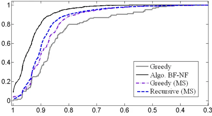
We first present numerical experiments with random graphs: for each density (0.1, 0.3, 0.5, 0.7 and 0.9), 100 bipartite graphs with 200 vertices (100 on each side, i.e., m = n = 100) were randomly
generated (the probability that an edge belongs to the graph is equal to the density). We then performed, for each graph, 100 runs with the same random initializations and each algorithm was allotted 100 iterations, except for the greedy heuristic which was always run until completion and only once for each graph (since it does not require a random initialization). Actual amounts of CPU time spent by Algorithms MS and BF-NF were comparable, as expected from their similar iteration complexity, while the greedy heuristic was faster.
Figure 2 displays the performance profile for these experiments [13], where the performance func-tion atρ≤1 is defined as the percentage, among all graphs and all runs, of bicliques whose sizes (i.e.
number of edges) is larger than ρ times the size the largest biclique found by any algortihm in the
corresponding graph, i.e.,
Figure 2: Performance profile for random graphs (densities from 0.1 to 0.9).
On such a performance profile, the higher the curve, the better ; more specifically, the left part of the graph measures efficiency, i.e. how often a given algorithm produces the best biclique among its peers, while the right part estimates robustness, i.e. how far from the best non-optimal solutions are. These two aspects are also reported more quantitatively in Table 1, which displays the value of the performance function atρ= 1 (Efficicency, i.e. how often a given algorithm find a biclique with largest
size) and the smallest value of ρ such that the performance function is equal to 100% (Robustness,
i.e. the relative size of the worst biclique found).
We observe on the performance profile that both Algorithm BF-NF and (MS) perform better than the greedy heuristic. The variant of (MS) using recursive post-processing performs slightly better than the one based on the use of the greedy heuristic. Nevertheless, Algorithm BF-NF generates in general better solutions: it is more efficient (9% of its solutions are ‘optimal’, twice better than the greedy (MS)) and more robust (all solutions are at most a factor 0.56 away from the best solution, better than 0.42 and 0.30 of other algorithms).
Densities Greedy Algo. 1 Greedy M.-S. Recursive M.-S. Both (Fig. 2) 1% — 0.42 9% — 0.56 4% — 0.30 2% — 0.30 Sparse (Fig. 3) 0% — 0.33 24% — 0.39 14% — 0.28 14% — 0.28 Dense (Fig. 3) 2% — 0.76 16% — 0.80 6% — 0.68 2% — 0.70
Table 1: Efficiency — Robustness.
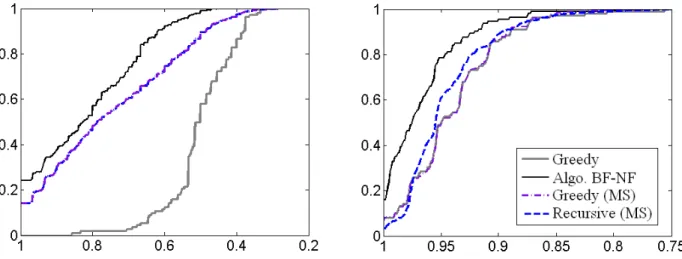
It is worth noting that the algorithms behave quite differently on sparse and dense graphs. Using the same setting as before, Figure 3 displays performance profiles for sparse graphs (on the left, with densities 0.05, 0.1, 0.15 and 0.2) and dense graphs (on the right, with densities 0.8, 0.85, 0.9 and 0.95). For sparse graphs, both versions of (MS) seem to coincide and the greedy heuristic performs significantly worse. For dense graphs, the greedy heuristic coincides with the greedy (MS) and performs almost as well as the recursive (MS). However, in all cases, Algorithm BF-NF performs better. It
Figure 3: Performance profiles for random graphs: sparse (left, from 0.05 to 0.2) and dense (right,
from 0.8 to 0.95).
is more efficient: it finds the best solution in 24% (resp. 16%) of the runs for sparse (resp. dense) graphs while (MS) only achieves 14% (resp. 6%) and the greedy heuristic 0% (resp. 2%). It is also more robust: all solutions are at most a factor 0.39 (resp. 0.80) away from the best solution for sparse (resp. dense) graphs, bigger than the best factor 0.33 (resp. 0.76) of the other algorithms.
Text Datasets
If parameterDin Algorithm BF-NF is chosen smaller than the value recommended by Corollary 1, the
algorithm is no longer guaranteed to converge to a biclique. However, the negative entries in Md will
force the corresponding entries of the solutions of (R1NF-MB) to be small (cf. Theorem 4). Therefore, instead of a biclique, one gets a dense submatrix of Mb, i.e., a bicluster. Algorithm BF-NF can then
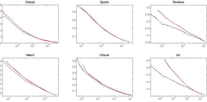
be used as abiclustering algorithm and the density of the corresponding submatrix will depend on the choice of parameter D between 0 and 2 max(m, n)|E|. We test this approach on the six text mining
datasets (with sparse matrices) described in Table 2.
Data m n |E| sparsity classic 7094 41681 223839 99.92 sports 8580 14870 1091723 99.14 reviews 4069 18483 758635 98.99 hitech 2301 10080 331373 98.57 ohscal 11162 11465 674365 99.47 la1 3204 31472 484024 99.52
Table 2: Text mining datasets [32] (sparsity is given in %: 100∗ |Z|/(mn)).
Figure 4 compares Algorithms BF-NF and MS for varying values of their parameters: for the Motzkin-Strauss formalism, we tested α = β ∈ [1.3,1.9] with step size 0.025 and, for Algorithm BF-NF, D ∈ d010[3,9] with step size 0.25 (d0 given by Equation (4.3)). For each value, we performed 10
runs (same initializations for both algorithms and 500 iterations) and plotted all the non-dominated solutions (i.e., for which no other solution has both larger size and higher density) for each dataset. We observe that our approach consistently generates better results since its curves dominate the ones
Figure 4: Normalized size vs. density for the Motzkin-Strauss formalism (dashed line) and Algo-rithm BF-NF based on (R1NF-MB) (solid line). The x-axis indicates the normalized sizes of the extracted clusters (i.e., number of entries in the extracted submatrix divided by the number of entries in the original matrix) while the y-axis indicates the density of these clusters (number of nonzero entries divided by the total number of entries) for the text datasets of Table 2.
of the Motzkin-Strauss formalism, i.e., the biclusters it finds are denser for the same size or larger for the same density.
Finally, we mention that Algorithm BF-NF can be further enhanced in the following ways:
• It is applicable to non-binary matrices, i.e., weighted graphs. Theorem 1 can easily be adapted
using d≥ ||M+||F (Lemma 1), and one can show that the resulting algorithm will converge to
the optimal rank-one approximation of a positive submatrix ofM.
• It is possible to give more weight to a given side of the biclique by adding regularization terms
to the cost functions. For example, on can consider the following objective function min
v,w≥0 ||Md−vw|| 2
F+α||v||22+β||w||22
which our algorithm can handle after some straightforward modifications (namely, the optimal solution for vwhenw is fixed can still be written in closed-form, and vice versa).
• If Mb ∈ {0,1}n×n is the adjacency matrix of a (non bipartite) graph G = (V, E) with V =
{v1, . . . , vn}, i.e.,Mb(i, j) = 1⇔(vi, vj)∈E, one can check that formulation (MB) corresponds
to the maximum edge biclique problem in any graph. This only requires that the diagonal entries of Mb are set to zero (no self loop in the graph) since a vertex cannot simultaneously belong
to both sides of a biclique. Therefore, all the results of this paper are actually valid for not necessarily bipartite graphs.
5
Conclusion
We have introduced Nonnegative Factorization (NF), a generalization of Nonnegative Matrix Factor-ization (NMF), and proved its NP-hardness in the rank-one case by reduction of the maximum edge
biclique problem. Since finding each rank-one factor in any NMF decomposition implicitly amounts to solving a rank-one NF problem, this suggests that (NMF) is a NP-hard problem for any fixed factoriza-tion rank and that no polynomial time algorithm based on the successive optimizafactoriza-tion of the rank-one factors can be designed, giving more credence to algorithms based on alternating optimization (e.g., the HALS algorithm or the standard alternating nonnegative least squares).
We also presented a heuristic algorithm for detecting large bicliques whose iterations requireO(|E|)
operations. It is based on results linking stationary points of a specific rank-one nonnegative factoriza-tion problem (R1NF-MB) and the maximum edge biclique problem. We experimentally demonstrated its efficiency and robustness on random graphs and text mining datasets.
References
[1] G. Alexe, S. Alexe, Y. Crama, S. Foldes, P.L. Hammer, and B. Simeone,Consensus algorithms
for the generation of all maximal bicliques, Discrete Applied Mathematics, 145(1) (2004), pp. 11–21.
[2] M. Berry, M. Browne, A. Langville, P. Pauca, and R.J. Plemmons,Algorithms and Applications
for Approximate Nonnegative Matrix Factorization, Computational Statistics and Data Analysis, 52 (2007),
pp. 155–173.
[3] M. Biggs, A. Ghodsi, and S. Vavasis,Nonnegative Matrix Factorization via Rank-One Downdate, in
25th international conference on machine learning (ICML), 2008.
[4] C. Cichocki and A-H. Phan, Fast local algorithms for large scale Nonnegative Matrix and Tensor
Factorizations, IEICE Transactions on Fundamentals of Electronics, Vol. E92-A No.3 (2009), pp. 708–721.
[5] C. Cichocki, R. Zdunek, and S. Amari,Hierarchical ALS Algorithms for Nonnegative Matrix and 3D
Tensor Factorization, in ICA07, London, UK, September 9-12, Lecture Notes in Computer Science, Vol.
4666, Springer, pp. 169-176, 2007.
[6] ,Nonnegative Matrix and Tensor Factorization, IEEE Signal Processing Magazine, (2008), pp. 142–
145.
[7] J.E. Cohen and U.G. Rothblum,Nonnegative ranks, Decompositions and Factorization of Nonnegative
Matrices, Linear Algebra and its Applications, 190 (1993), pp. 149–168.
[8] K. Devarajan,Nonnegative Matrix Factorization: An Analytical and Interpretive Tool in Computational
Biology, PLoS Computational Biology, 4(7), e1000029 (2008).
[9] I.S. Dhillon and S. Sra,Nonnegative Matrix Approximations: Algorithms and Applications, tech. report,
University of Texas (Austin), 2006. Dept. of Computer Sciences.
[10] C. Ding, X. He, and H.D. Simon,On the Equivalence of Nonnegative Matrix Factorization and Spectral
Clustering, in SIAM Int’l Conf. Data Mining (SDM’05), 2005, pp. 606–610.
[11] C. Ding, T. Tao L, and M.I. Jordan,Nonnegative matrix factorization for combinatorial optimization:
Spectral clustering, graph matching, and clique finding, Data Mining, IEEE International Conference on,
(2008), pp. 183–192.
[12] C. Ding, Y. Zhang, T. Li, and S.R. Holbrook, Biclustering Protein Complex Interactions with a
Biclique Finding Algorithm, in Sixth IEEE International Conference on Data Mining, 2006, pp. 178–187.
[13] E.D. Dolan and J.J. Mor´e, Benchmarking optimization software with performance profiles, Math.
Program., Ser. A, 91 (2002), pp. 201–213.
[14] N. Gillis,Approximation et sous-approximation de matrices par factorisation positive: algorithmes,
com-plexit´e et applications, master’s thesis, Universit´e catholique de Louvain, 2007. In French.
[15] N. Gillis and F. Glineur, Using underapproximations for sparse nonnegative matrix factorization,
Pattern Recognition, 43(4) (2010), pp. 1676–1687.
[16] L. Grippo and M. Sciandrone,On the convergence of the block nonlinear Gauss-Seidel method under
[17] N.-D. Ho, Nonnegative Matrix Factorization - Algorithms and Applications, PhD thesis, Universit´e
catholique de Louvain, 2008.
[18] P.O. Hoyer, Nonnegative Matrix Factorization with Sparseness Constraints, J. Machine Learning
Re-search, 5 (2004), pp. 1457–1469.
[19] H. Kim and H. Park, Non-negative Matrix Factorization Based on Alternating Non-negativity
Con-strained Least Squares and Active Set Method, SIAM J. Matrix Anal. Appl., 30(2) (2008), pp. 713–730.
[20] J. Kim and H. Park, Sparse Nonnegative Matrix Factorization for Clustering, Tech. Report
GT-CSE-08-01, Georgia Institute of Technology, 2008.
[21] D.D. Lee and H.S. Seung,Learning the Parts of Objects by Nonnegative Matrix Factorization, Nature,
401 (1999), pp. 788–791.
[22] , Algorithms for Non-negative Matrix Factorization, In Advances in Neural Information Processing,
13 (2001).
[23] C.-J. Lin, Projected Gradient Methods for Nonnegative Matrix Factorization, Neural Computation, 19
(2007), pp. 2756–2779. MIT press.
[24] G. Liu, K. Sim, and J. Li,Efficient Mining of Large Maximal Bicliques, Springer Berlin, Lecture Notes
in Computer Science, (2006), pp. 437–448.
[25] P. Miettinen,The boolean column and column-row matrix decompositions, Data Mining and Knowledge
Discovery, 17(1) (2008), pp. 39–56.
[26] P. Paatero and U. Tapper, Positive matrix factorization: a non-negative factor model with optimal
utilization of error estimates of data values, Environmetrics, 5 (1994), pp. 111–126.
[27] R. Peeters,The maximum edge biclique problem is NP-complete, Discrete Applied Mathematics, 131(3)
(2003), pp. 651–654.
[28] G.W. Stewart and J.-g. Sun,Matrix Perturbation Theory, Academic Press, San Diego, 1990.
[29] S.A. Vavasis,On the complexity of nonnegative matrix factorization, SIAM Journal on Optimization, 20
(2009), pp. 1364–1377.
[30] Z.-Y. Zhang, T. Li, C. Ding, X.W. Ren, and X.-S. Zhang,Binary matrix factorization for analyzing
gene expression data, Data Mining and Knowledge Discovery, 20 (1) (2009), pp. 28–52.
[31] Z.-Y. Zhang, T. Li, C. Ding, and X.-S. Zhang, Binary matrix factorization with applications, in
Proceedings of 2007 IEEE International Conference on Data Mining (ICMD07), 2007.
[32] S. Zhong and J. Ghosh,Generative model-based document clustering: a comparative study, Knowledge
Recent titles
CORE Discussion Papers
2010/20. Jeroen V.K. ROMBOUTS and Lars STENTOFT. Multivariate option pricing with time varying volatility and correlations.
2010/21. Yassine LEFOUILI and Catherine ROUX. Leniency programs for multimarket firms: The effect of Amnesty Plus on cartel formation.
2010/22. P. Jean-Jacques HERINGS, Ana MAULEON and Vincent VANNETELBOSCH. Coalition formation among farsighted agents.
2010/23. Pierre PESTIEAU and Grégory PONTHIERE. Long term care insurance puzzle.
2010/24. Elena DEL REY and Miguel Angel LOPEZ-GARCIA. On welfare criteria and optimality in an endogenous growth model.
2010/25. Sébastien LAURENT, Jeroen V.K. ROMBOUTS and Francesco VIOLANTE. On the forecasting accuracy of multivariate GARCH models.
2010/26. Pierre DEHEZ. Cooperative provision of indivisible public goods.
2010/27. Olivier DURAND-LASSERVE, Axel PIERRU and Yves SMEERS. Uncertain long-run emissions targets, CO2 price and global energy transition: a general equilibrium approach. 2010/28. Andreas EHRENMANN and Yves SMEERS. Stochastic equilibrium models for generation
capacity expansion.
2010/29. Olivier DEVOLDER, François GLINEUR and Yu. NESTEROV. Solving infinite-dimensional optimization problems by polynomial approximation.
2010/30. Helmuth CREMER and Pierre PESTIEAU. The economics of wealth transfer tax.
2010/31. Thierry BRECHET and Sylvette LY. Technological greening, eco-efficiency, and no-regret strategy.
2010/32. Axel GAUTIER and Dimitri PAOLINI. Universal service financing in competitive postal markets: one size does not fit all.
2010/33. Daria ONORI. Competition and growth: reinterpreting their relationship.
2010/34. Olivier DEVOLDER, François GLINEUR and Yu. NESTEROV. Double smoothing technique for infinite-dimensional optimization problems with applications to optimal control.
2010/35. Jean-Jacques DETHIER, Pierre PESTIEAU and Rabia ALI. The impact of a minimum pension on old age poverty and its budgetary cost. Evidence from Latin America.
2010/36. Stéphane ZUBER. Justifying social discounting: the rank-discounting utilitarian approach. 2010/37. Marc FLEURBAEY, Thibault GAJDOS and Stéphane ZUBER. Social rationality, separability,
and equity under uncertainty.
2010/38. Helmuth CREMER and Pierre PESTIEAU. Myopia, redistribution and pensions.
2010/39. Giacomo SBRANA and Andrea SILVESTRINI. Aggregation of exponential smoothing processes with an application to portfolio risk evaluation.
2010/40. Jean-François CARPANTIER. Commodities inventory effect.
2010/41. Pierre PESTIEAU and Maria RACIONERO. Tagging with leisure needs.
2010/42. Knud J. MUNK. The optimal commodity tax system as a compromise between two objectives. 2010/43. Marie-Louise LEROUX and Gregory PONTHIERE. Utilitarianism and unequal longevities: A
remedy?
2010/44. Michel DENUIT, Louis EECKHOUDT, Ilia TSETLIN and Robert L. WINKLER. Multivariate concave and convex stochastic dominance.
2010/45. Rüdiger STEPHAN. An extension of disjunctive programming and its impact for compact tree formulations.
2010/46. Jorge MANZI, Ernesto SAN MARTIN and Sébastien VAN BELLEGEM. School system evaluation by value-added analysis under endogeneity.
2010/47. Nicolas GILLIS and François GLINEUR. A multilevel approach for nonnegative matrix factorization.
2010/48. Marie-Louise LEROUX and Pierre PESTIEAU. The political economy of derived pension rights.
2010/49. Jeroen V.K. ROMBOUTS and Lars STENTOFT. Option pricing with asymmetric heteroskedastic normal mixture models.
Recent titles
CORE Discussion Papers - continued
2010/50. Maik SCHWARZ, Sébastien VAN BELLEGEM and Jean-Pierre FLORENS. Nonparametric frontier estimation from noisy data.
2010/51. Nicolas GILLIS and François GLINEUR. On the geometric interpretation of the nonnegative rank.
2010/52. Yves SMEERS, Giorgia OGGIONI, Elisabetta ALLEVI and Siegfried SCHAIBLE. Generalized Nash Equilibrium and market coupling in the European power system.
2010/53. Giorgia OGGIONI and Yves SMEERS. Market coupling and the organization of counter-trading: separating energy and transmission again?
2010/54. Helmuth CREMER, Firouz GAHVARI and Pierre PESTIEAU. Fertility, human capital accumulation, and the pension system.
2010/55. Jan JOHANNES, Sébastien VAN BELLEGEM and Anne VANHEMS. Iterative regularization in nonparametric instrumental regression.
2010/56. Thierry BRECHET, Pierre-André JOUVET and Gilles ROTILLON. Tradable pollution permits in dynamic general equilibrium: can optimality and acceptability be reconciled?
2010/57. Thomas BAUDIN. The optimal trade-off between quality and quantity with uncertain child survival.
2010/58. Thomas BAUDIN. Family policies: what does the standard endogenous fertility model tell us? 2010/59. Nicolas GILLIS and François GLINEUR. Nonnegative factorization and the maximum edge
biclique problem.
Books
J. GABSZEWICZ (ed.) (2006), La différenciation des produits. Paris, La découverte.
L. BAUWENS, W. POHLMEIER and D. VEREDAS (eds.) (2008), High frequency financial econometrics: recent developments. Heidelberg, Physica-Verlag.
P. VAN HENTENRYCKE and L. WOLSEY (eds.) (2007), Integration of AI and OR techniques in constraint programming for combinatorial optimization problems. Berlin, Springer.
P-P. COMBES, Th. MAYER and J-F. THISSE (eds.) (2008), Economic geography: the integration of regions and nations. Princeton, Princeton University Press.
J. HINDRIKS (ed.) (2008), Au-delà de Copernic: de la confusion au consensus ? Brussels, Academic and Scientific Publishers.
J-M. HURIOT and J-F. THISSE (eds) (2009), Economics of cities. Cambridge, Cambridge University Press. P. BELLEFLAMME and M. PEITZ (eds) (2010), Industrial organization: markets and strategies. Cambridge
University Press.
M. JUNGER, Th. LIEBLING, D. NADDEF, G. NEMHAUSER, W. PULLEYBLANK, G. REINELT, G. RINALDI and L. WOLSEY (eds) (2010), 50 years of integer programming, 1958-2008: from the early years to the state-of-the-art. Berlin Springer.
CORE Lecture Series
C. GOURIÉROUX and A. MONFORT (1995), Simulation Based Econometric Methods. A. RUBINSTEIN (1996), Lectures on Modeling Bounded Rationality.
J. RENEGAR (1999), A Mathematical View of Interior-Point Methods in Convex Optimization.
B.D. BERNHEIM and M.D. WHINSTON (1999), Anticompetitive Exclusion and Foreclosure Through Vertical Agreements.
D. BIENSTOCK (2001), Potential function methods for approximately solving linear programming problems: theory and practice.
R. AMIR (2002), Supermodularity and complementarity in economics. R. WEISMANTEL (2006), Lectures on mixed nonlinear programming.