Archive University of Zurich Main Library Strickhofstrasse 39 CH-8057 Zurich www.zora.uzh.ch Year: 2015
Location and density of rain gauges for the estimation of spatial varying
precipitation
Girons Lopez, Marc ; Wennerström, Hjalmar ; Nordén, Lars-Åke ; Seibert, Jan
Abstract: Accurate estimation of precipitation and its spatial variability is crucial for reliable discharge simula- tions. Although radar and satellite based techniques are becoming increasingly widespread, quantitative precipita- tion estimates based on point rain gauge measurement inter- polation are, and will continue to be in the foreseeable future, widely used. However, the ability to infer spatially dis-tributed data from point measurements is strongly dependent on the number, location and reliability of meas- urement stations. In this study we quantitatively investigated the effect of rain gauge network configurations on the spatial interpola- tion by using the operational hydrometeorological sensor network in the Thur river basin in north-eastern Switzerland as a test case. Spatial precipitation based on a combination of radar and rain gauge data provided by MeteoSwiss was assumed to represent the true precipitation values against which the precipitation interpolation from the sensor network was evaluated. The performance using scenarios with both increased and decreased station density were explored. The catchment-average interpolation error indices significantly improve up to a density of 24 rain gauges per 1000 km2, beyond which improvements were negligible. However, a reduced rain gauge density in the higher parts of the catchment resulted in a noticeable decline of the perfor- mance indices. An evaluation based on precipitation inten- sity thresholds indicated a decreasing performance for higher precipitation intensities. The results of this study emphasise the benefits of dense and adequately distributed rain gauge networks.
DOI: https://doi.org/10.1111/geoa.12094
Posted at the Zurich Open Repository and Archive, University of Zurich ZORA URL: https://doi.org/10.5167/uzh-112590
Journal Article Published Version Originally published at:
Girons Lopez, Marc; Wennerström, Hjalmar; Nordén, Lars-Åke; Seibert, Jan (2015). Location and density of rain gauges for the estimation of spatial varying precipitation. Geografiska Annaler: Series A, Physical Geography, 97(1):167-179.
LOCATION AND DENSITY OF RAIN GAUGES FOR THE
ESTIMATION OF SPATIAL VARYING PRECIPITATION
MARC GIRONS LOPEZ1, HJALMAR WENNERSTRÖM2, LARS-ÅKE NORDÉN2and JAN SEIBERT1,3
1Department of Earth Sciences, Uppsala University, Uppsala, Sweden 2Department of Information Technology, Uppsala University, Uppsala, Sweden
3Department of Geography, University of Zurich, Zurich, Switzerland
Girons Lopez, M., Wennerström, H., Nordén, L.-Å. and Seibert, J., 2015. Location and density of rain gauges for the estimation of spatial varying precipitation. Geografiska Annaler: Series A, Physical Geography, 97, 167–179.
doi:10.1111/geoa.12094
ABSTRACT. Accurate estimation of precipitation and its spatial variability is crucial for reliable discharge simula-tions. Although radar and satellite based techniques are becoming increasingly widespread, quantitative precipita-tion estimates based on point rain gauge measurement inter-polation are, and will continue to be in the foreseeable future, widely used. However, the ability to infer spatially distributed data from point measurements is strongly dependent on the number, location and reliability of meas-urement stations.
In this study we quantitatively investigated the effect of rain gauge network configurations on the spatial interpola-tion by using the operainterpola-tional hydrometeorological sensor network in the Thur river basin in north-eastern Switzerland as a test case. Spatial precipitation based on a combination of radar and rain gauge data provided by MeteoSwiss was assumed to represent the true precipitation values against which the precipitation interpolation from the sensor network was evaluated. The performance using scenarios with both increased and decreased station density were explored. The catchment-average interpolation error indices significantly improve up to a density of 24 rain gauges per 1000 km2, beyond which improvements were negligible.
However, a reduced rain gauge density in the higher parts of the catchment resulted in a noticeable decline of the perfor-mance indices. An evaluation based on precipitation inten-sity thresholds indicated a decreasing performance for higher precipitation intensities. The results of this study emphasise the benefits of dense and adequately distributed rain gauge networks.
Key words: precipitation monitoring, point measurements, sensor networks, interpolation
Introduction
Precipitation is one of the main components of the global hydrological cycle and the most important
driving input for stream flow. Knowing when, where, and how much precipitation might occur is of interest for many aspects of human society and crucial for water management. While for some applications an average estimation of the pre-cipitation might be enough, for others such as (semi-)distributed hydrological modelling and forecasting, knowing the spatial and temporal dis-tribution of precipitation is of crucial interest (Goodrich et al. 1995; Schuurmans and Bierkens 2007). This is especially due to the often high spatial variability of precipitation, which can intro-duce large uncertainties in hydrological predictions (Chowet al. 1988).
Until recently, interpolation of point measure-ments from rain gauges has been the only option to obtain spatial precipitation information. In recent years different spatial measurement techniques such as Doppler weather radars and satellite imaging have been developed and have progres-sively been incorporated into operational settings (Savvidouet al. 2009; Priceet al. 2013). However, the coarse resolution of satellite images, and problems with radar signal interpretation mean that point measurements are still widely used in combination with radar data (for calibration and validation purposes) or as the only source of information in areas with no radar coverage (Messeret al. 2006; Voglet al. 2012; Priceet al. 2013).
Spatial precipitation estimation from point measurements is subject to two main sources of uncertainties, the errors with the measurements themselves and the estimation of the spatial and temporal precipitation variability (McMillanet al. 2012). In this study the latter is addressed. Regard-ing precipitation inter- and extrapolation from point measurements, many different methods are
available (see Haberlandt 2011 for a review). However, even with the most sophisticated inter-polation methods based on dense rain gauge net-works there might be significant errors in the mean areal precipitation, especially at the smallest scales (McMillan et al. 2012). Wood et al. (2000) and Goodrich et al. (1995) show that precipitation interpolation uncertainties rapidly escalate with increasing interpolation resolution due to the higher precipitation variability when averaging over smaller areas. For their specific study, Goodrichet al. (1995) found an increase from 4% to 14% at a 102m scale to over 65% at a 104m
scale.
The necessary rain gauge density depends to a large extent on the objectives of the data collection (i.e. desired degree of accuracy), on the local spatial variability of the precipitation, and the char-acteristics of individual catchment (Jones 1997; Tilfordet al. 2003). Optimal densities are difficult to achieve in reality due to various practical constraints such as lack of funding and limited accessibility as well as lack of knowledge on the local precipitation variability. For these reasons, minimum rain gauge density guidelines have been established for different settings and monitoring objectives (WMO 2008). Even so, inadequate coverage and sustainability of monitoring net-works continues to be one of the main issues for crucial water management practices, such as flood warning systems, with the exception of some major river basins (UN 2006; WMO 2011).
Several studies have investigated the perfor-mance of rain gauge networks to estimate precipi-tation spatial distribution in a large range of geographical settings and temporal and spatial scales. In a study on rainfall measurement accuracy for hydrological purposes, Wood et al. (2000) determined that radar estimates were generally more accurate than rain gauge estimates for esti-mating rainfall at a catchment scale. In a similar study, Xuet al. (2013) found that the error range of rain gauge precipitation estimates for increasing network densities reach a threshold beyond which no considerable improvements are seen. Balme
et al. (2006) showed that rain gauge density
decline in a larger area produces a significant increase in spatial rainfall estimation errors at annual scales and even larger errors at event scales. Other studies have addressed the issue of how to improve the spatial precipitation estimation from point measurements. A good example is the work by Clark and Slater (2006) in which they explored
the use of spatial attributions from station locations to generate precipitation estimates in complex ter-rains. Several authors have studied the effect of precipitation estimates from rain gauges in wider contexts, such as for hydrological modelling. For instance, Biggs and Atkinson (2011) found that six rain gauges in the Severn Uplands (UK) could be used to predict flows with a similar accuracy as with radar data. Schuurmans and Bierkens (2007) studied the influence of precipitation variability on the hydrological behaviour of a catchment in the Netherlands through standardised non-zero rainfall variograms. Bárdossy and Das (2008) investigated the influence of precipitation spatial resolution on hydrological model calibration by varying the dis-tribution of a rain gauge network in a mesoscale catchment in Germany. Focusing on hydrological forecasts, Anctil et al. (2006) tried to improve rainfall-runoff forecasts by optimising mean daily area rainfall time series and evaluated the impact of reduced rainfall knowledge by using thegoodness
of rainfall estimation (GORE) and BALANCE
indices proposed by Andréassianet al. (2001). In this paper we present a study on the reliability of different rain gauge sensor network configura-tions for spatial precipitation estimation at a catch-ment scale. The data from an operational rain gauge sensor network were used as the base network configuration and variations based on the interpolation evaluation were implemented. Differ-ent scenarios were considered regarding both the impact of including additional rain gauges as well as removing subsets of the existing rain gauges. High-resolution time series data of precipitation fields combining rain gauge and radar data (MeteoSwiss 2013b) were used as evaluation ref-erence as a best estimate of the true precipitation. The data available allowed a quantitative evalua-tion based on the precipitaevalua-tion estimaevalua-tion errors and based on the estimation of precipitation inten-sity thresholds.
Study area and dataset
The study was carried out for the Thur basin, a medium-sized (∼1700 km2) basin in north-eastern
Switzerland with a mean altitude of about 770 m a.s.l. (Fig. 1). The Thur river is the largest non-regulated river in Switzerland and drains the front ranges of the Swiss Alps (PEER 2010). The catchment is fairly densely populated with St Gallen and Frauenfeld being the largest urban con-centrations (FSO 2013).
Precipitation in the Thur basin is distributed relatively evenly over the year with the largest volumes and intensities occurring during the summer ((MeteoSwiss 2014a). The mean annual precipitation is 1350 mm yr–1, ranging from about
950 mm yr–1 in the northern lowlands to over
2000 mm yr–1 in southern pre-alpine headwaters.
The Thur river is strongly influenced by snow-melt and large rain events in the headwaters may cause rapid increases of discharge. The mean flow over the period 1904–2008 was about 47 m3s–1, which
corresponds to 870 mm yr–1(FOEN 2013). During
the last century, at least three events producing flows higher than 1000 m3s–1have been recorded
(in the years 1910, 1978 and 1999).
The Swiss Federal Office of Meteorology and Climatology (MeteoSwiss) operates a high-resolution manual precipitation monitoring network over the whole country which provides daily data (MeteoSwiss 2014b). A number of these stations will be replaced in the near future by auto-matic rain gauges providing measurements every 10 min (MeteoSwiss, http://www.MeteoSwiss .admin.ch/web/en/climate/observation_systems/ surface/swissmetnet.html, 1 Feb., 2014). Addition-ally, since 2005, MeteoSwiss has been progressively deploying a network of automatic meteorological monitoring stations (SwissMetNet) measuring several meteorological parameters such
as temperature, humidity, air pressure, wind direc-tion and speed, precipitadirec-tion and radiadirec-tion. Most of these stations are already operational and transfer measured data at 10 min intervals (Suter et al. 2006). The spatial distribution of the available meteorological stations is reasonably balanced but high altitudes (above 1200 m a.s.l.) remain under-represented as rain gauges tend to be placed at low elevations where there is a higher population density (Frei and Schär 1998). This bias, when combined with the general mean precipitation increase with altitude (Peck and Brown 1962), can result in a systematic underestimate of precipita-tion. In addition to the ground precipitation obser-vation stations, three radar stations used for monitoring and forecasting precipitation events over the whole country have been operational for approximately 20 years (Joss et al. 1997). The radar network has recently been renewed and expanded with the construction of a new radar station at La Plaine Morte, Valais (MeteoSwiss 2013c).
MeteoSwiss also develops several grid-data products based on the collected meteorological data, two of which were of special interest for the present study. The first product, RhiresD, is a spatial analysis of daily precipitation totals extend-ing over a long period (1961–present) built on the data from all the available station measurements at a certain day at a spatial resolution of 0° 1′15″
(MeteoSwiss 2013a). The other product, named RdisaggH, is a combination of the rain-gauge-based high-resolution interpolation data from RhiresD and an hourly composite of radar meas-urements (NASS) (MeteoSwiss 2013b). The aggre-gation of the two data sources allows for a very high resolution both at the temporal scale (1 h) and at the spatial scale (1 km2). Currently this product,
however, is only available for the period May 2003 to December 2010.
The extent of the study was defined by the Thur catchment and the data availability. A gridded area of 80×80 km was defined around the catchment with a resolution of 4 km2. By considering a larger
area than the Thur catchment (for which the evalu-ation was carried out), surrounding rain gauges were also incorporated in the interpolation proce-dure to ensure an adequate coverage of all parts of the catchment including its borders. The only exception was the north-western edge of the catch-ment, which lies at a short distance from the national border (the limit of the area covered by MeteoSwiss data and products). The study area
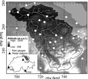
Fig. 1. Geographical location of the Thur catchment. The grey scale map represents the terrain elevation data and the main rivers and lakes (hatched areas). The coordinates are expressed in the CH1903 Swiss coordinate system. The rain gauge locations represent the manual rain gauges operated by MeteoSwiss that are used for this study. Source: Swiss Federal Office of Topography.
included 60 MeteoSwiss manual pluviometric sta-tions, 21 of which lie within the catchment (Fig. 1). The corresponding rain gauge density is 12 stations per 1000 km2, which is much higher than the
rec-ommended minimum density from mountainous areas (four stations per 1000 km2; WMO 2008).
Since the analysis depended on the RdisaggH data product, the temporal extent of the study was con-strained by the period for which this data were available, providing approximately 8 years of data. Even if this time period was short it captured a wide range of precipitation events, including five events that caused floods larger than the 5-year flood. A dataset consisting of the 500 h with highest precipitation volumes in 10% of the catch-ment area was selected as the analysis period. Con-sequently, the periods with lowest precipitation intensities (or no recorded precipitation) were effectively excluded from the analysis. The result-ing dataset had an adequate sample size and wide range of precipitation variability, and included the previously mentioned precipitation peaks (Fig. 2).
Methods
The evaluation of different rain gauge sensor network configurations for spatial precipitation interpolation required the spatial distribution and magnitude of the real precipitation to be known. Since this is obviously unknown, a surrogate evaluation reference was used. In this case, the RdisaggH data product provided a valuable approximation of the real precipitation pattern given its temporal and spatial resolution and good representation of both rainfall spatial distribution and volumes, which made it an appropriate evalu-ation reference dataset. However, even if the Rdis-aggH data product is a good estimate of the real
precipitation, its errors and uncertainties need to be taken into account in order to constrain the limita-tions of the study. The main issues of this data product are an overall small positive bias as well as a systematic underestimation of high precipitation intensities and an overestimation of low intensities (MeteoSwiss 2013b). Other inaccuracies arise from the topographic shielding of the radar beam in mountainous areas.
A subset of the RdisaggH data product only including data at the location of the existing manual precipitation monitoring stations was used to obtain the data series of the rain gauges at an hourly interval instead of at the daily interval in which these data are actually collected. The higher temporal resolution compared with the actual sta-tions allowed reproducing short and intense pre-cipitation events that would otherwise be missed with the original data collection intervals (daily). This assumption was considered valid as the evalu-ation was done for the interpolated grid cells and not for the station locations, which avoided the issue of evaluating the interpolation with the same data from which it was generated. Additionally, a scenario where most monitoring stations would have hourly collection intervals was considered plausible due to the increasing number of auto-matic stations with hourly and even sub-hourly temporal resolution being made available in the area.
Precipitation interpolation methodology
The interpolation method applied was based on the methodology used for the creation of the RhiresD data product (MeteoSwiss 2013a). Using the same interpolation approach ensured robustness in the methodology and allowed for a more consistent
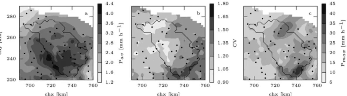
Fig. 2. Precipitation statistics for the Thur catchment over the study period. (a) Average precipitation (mm h–1). (b) Coefficient of
variation (CV). (c) Maximum registered precipitation (mm h–1). The coordinates are expressed in the CH1903 Swiss coordinate
verification of the results and their uncertainties. This methodology can be divided into three main steps. First, the relative anomalies (precipitation difference over reference precipitation) of the station measurements with respect to the monthly long-term climatological average were calculated for every time step (hour) of the study period. This was done in order to reduce the bias resulting from interpolating in a region with large elevation dif-ferences (Freiet al. 2006). The reference precipi-tation used for this study was a long-term monthly climatological average based on regionally varying precipitation–topography relationships adjusted for the Alpine region (Schwarbet al. 2001). The relative anomalies were then interpolated for the whole study area using a modified version of the SYMAP algorithm (Shepard 1968). The result-ing anomaly field was finally multiplied by the climatological average in order to get the final pre-cipitation values.
The SYMAP algorithm has been previously used in many studies and has been found to perform equally well as kriging methods (Weber and Englund 1992). SYMAP is an inverse-distance weighting interpolation method that estimates the value of a grid point,u(x), based on the values of several neighbouring observations or data points,
ui, using a weighting function,wi(Eqn 1).
u x w u w i i i n i i n
( )
= =(
∗)
=∑
∑
1 1 (1)The weighting function is a product of the distance weights,si, and the sum of one and the directional weights,ti, of the surrounding observations which effectively down-weights both distant and clus-tered observations (Eqn 2).
wi=si2
(
1+ti)
(2) In this study we used a modification of the origi-nal distance weighting function by Frei and Schär (1998) that omits the gradient corrections in order to ensure consistency with the approach taken for RhiresD. The weighting function uses a scaled distance function, ri, to determine the size of the search area and the weight of observations. The distance between the grid point (xg,yg) and the observations (xo,yo) is scaled using a multiple,i=(1,2,3,4), of the predefined mesh size (Δx,Δy). The distance weighting function has the
final form of:
s r r r i i i i =
(
+(
∗)
)
≤ > 1 2 1 0 1 cos , , π (3) where ri=(
(
x0−xg)
i x)
+(
(
y −yg)
i y)
2 0 2 ∆ ∆ (4)Finally, the directional weighting function depends on the weights of the other data points,sj, within the search area, and the angle,θ, between
the grid point, the considered observation, and the other data points:
t s s i j j m j j m = −
( )
(
)
= =∑
∑
1 1 1 cosθ (5)In the present study the basic search radius was set at 5 km. This value was chosen based on the rain gauge density and was a compromise between using only local data for the interpolation and having enough data points to perform the interpo-lation successfully.
Precipitation interpolation evaluation
An evaluation of the aforementioned interpolation method performed by MeteoSwiss (2013a) showed that precipitation magnitudes were under-estimated for high precipitation intensities and overestimated for low intensities, with the largest errors occurring during summer periods and for localised thunderstorms. The magnitude of the errors derived from the interpolation method was also found to be strongly dependent on the inter-pretation of the interpolated grid-cell values. If interpolated cell values are assumed to represent point estimates of the precipitation, errors were found to be large. However, if such values were assumed to represent an average precipitation over a larger area the magnitudes of the errors were significantly reduced. For this reason they claim that the effective resolution of the interpo-lation is of the order of 15–20 km. Following the conclusions of this investigation, for the present study the performance of the different rain gauge sensor network configurations was evaluated both at a grid-cell resolution (4 km2) and at a lower
resolution (36 km2) in order to test the
Error estimation and sensor network
configura-tions The precipitation estimation errors were
quantitatively determined in a distributed way for both of the previously mentioned resolutions as well as averaged over the entire catchment. Two different indices were used to estimate the interpolation errors: thePearson correlation coef-ficient(IPCC), and thenormalised root-mean-square error(IRMSE), which are expressed in the following way: I P P P P P P P P PCC t s s t o o t n t s s t o o t n = −
(
)
(
−)
−(
)
(
−)
= =∑
∑
, , , , 1 2 2 1 (6) I P P n P P RMSE t s t o t n max o min o = −(
)
− =∑
, , , , 2 1 (7)wherePt,sandPt,oare the simulated and observed precipitation values per time step,Pmax,oandPmin,o
the maximum and minimum observed values, and
Psand Poare the respective mean values over time. The different error indices were used in order to evaluate different aspects of the precipitation field, such as the rainfall variability or the outliers (large magnitude events).
Sensor network configurations Two different sce-narios were considered for testing the performance of different rain gauge sensor network configura-tions. The first scenario tested the interpolation per-formance for increased sensor network densities. In this scenario one station was added at a time for both interpolation resolutions, considering the best case scenario where the new station would be placed at the location with the highest interpolation error. This process was repeated iteratively until 40 hypothetical rain gauges were added to the network. The other scenario represented a decrease in the sensor network density. For this scenario the stations situated above 800 m a.s.l. were succes-sively removed from the analysis in decreasing elevation order. Most of the rain gauges above the considered altitude were among the most recently deployed as such areas are the least accessible. The importance of this subset of the rain gauges lies in that they are located in the areas that record the highest precipitation volumes and variability of the entire catchment (Fig. 2b, c).
Precipitation threshold estimation The rain
gauge sensor network configurations created with the different indexes were also evaluated on the basis of their capacity to reproduce different pre-cipitation intensity thresholds. The evaluation of the precipitation threshold estimation was done by calculating an efficiency rate defined by the number of times the threshold level was estimated correctly divided by the number of times the threshold level was actually reached. This evalua-tion was performed separately for the two different thresholds of 5 and 10 mm h–1. The higher
thresh-old was defined as the highest hourly precipitation value that was found to occur in each single grid cells in the catchment (Fig. 2c) and the lower threshold was chosen as half of this intensity.
Results
Precipitation interpolation error estimation
The evaluation of the existing rain gauge sensor network with the different error indices and at the different resolutions showed that for both indices errors were generally lower and smoother when evaluated at the lower resolution (36 km2) (Fig. 3).
The spatial distribution of the errors was similar between the different indices, with the lower per-formance located at the areas with lower rain gauge densities, especially at the south-western edge of the basin as well as a large area in the north-eastern side.
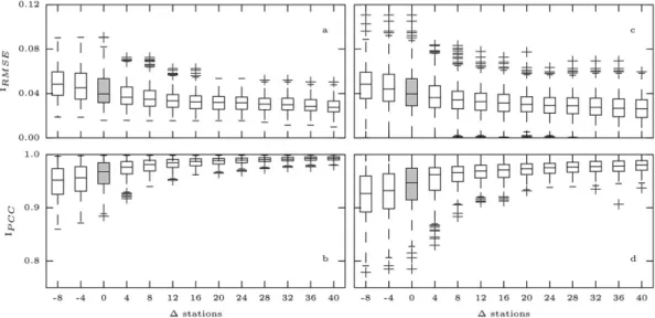
The error magnitudes change significantly when the station density in the catchment was modified (Fig. 4). Catchment average performance mean and ranges tend to be larger and more variable for the higher interpolation resolution (4 km2) in a
similar way as for distributed errors (Fig. 3). The evolution of the different error indices for the dif-ferent rain gauge densities considered was compa-rable. There was an overall tendency for the error mean and range to decrease with increasing rain gauge density and to increase with decreasing density. The error reduction followed approxi-mately an exponential decay where the achieved error reduction of adding a new station was pro-gressively lower until a plateau was reached. After inclusion of about 20 hypothetical stations, result-ing in a density of 24 rain gauges per 1000 km2, the
error average and variation changes were insignifi-cant for both error indices.
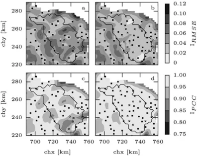
The performance of rain gauge network configu-rations with densities of eight and 24 rain gauges per 1000 km2, representing the removal of eight
rain gauges and the inclusion of 20 rain gauges respectively, showed that for the scenario involving a lower station density at high elevations, the errors increased noticeably for the southern part of the basin (Fig. 5). However, after the addition of 20 hypothetical stations, the higher density combined
with a more uniform distribution of the rain gauges resulted in generally small errors.
A comparison of the location of 20 hypothetical rain gauges using the different error indices is pre-sented in Fig. 6a. The placement of the hypotheti-cal rain gauges was similar for both indices (in
Fig. 3. Performance of the existing rain gauge network configuration for different indicators and interpolation resolutions. (a) IRMSEat
36 km2resolution. (b) I
RMSEat 4 km2resolution. (c) IPCCat 36 km2resolution. (d) IPCCat 4 km2resolution. The individual rain gauges
are represented as solid squares and the coordinates are expressed in the CH1903 Swiss coordinate system.
Fig. 4. Catchment average performance (mean and range) for different rain gauge network configurations generated by adding and removing measurement stations at different interpolation resolutions. (a) IRMSEat 36 km2resolution. (b) IRMSEat 4 km2resolution. (c)
several cases the locations are overlapping) and tended to cover the areas with lower rain gauge density in the existing sensor network. Most of the additional rain gauges were placed in the areas
along the water divide, especially in the southern edge of the catchment, which corresponds to the highest precipitation amounts and variability. Using theIPCCindex tended to place more stations
Fig. 5. Performance of two characteristic rain gauge network configurations interpolated at a resolution of 36 km2for different
indicators. (a) IRMSEafter the removal of eight rain gauges. (b) IRMSEafter the placement of 20 hypothetical rain gauges. (c) IPCCafter
the removal of eight rain gauges. (d) IPCCafter the placement of 20 hypothetical rain gauges. The existing rain gauge network is
represented by the solid squares, the stations removed by empty circles, and the stations added by crosses. The coordinates are expressed in the CH1903 Swiss coordinate system.
Fig. 6. (a) Location of the hypothetical rain gauges placed according to the two error indices when a density of 24 stations per 1000 km2is reached. (b) I
RMSEmagnitude as a function of the distance between all grid cells in the Thur catchment and their closest
rain gauge for different network configurations. (c) IPCCmagnitude as a function of the distance between all grid cells in the Thur
catchment and their closest rain gauge for different network configurations. The coordinates in (a) are expressed in the CH1903 Swiss coordinate system.
at the lower parts of the catchment compared with theINRMSE, which resulted in more rain gauges at the middle parts of the catchment.
The relationship between the different error indices and the distance of each grid-cell in the basin to its closest rain gauge is explored in Fig. 6b,c for increasingly dense rain gauge network configurations. The distance from each grid cell to the closest station obviously decreased with increasing station density but more importantly, there was a clear correlation between error magni-tude and distance to the closest rain gauge station. Interestingly, the gradient of this correlation decreased for denser network configurations.
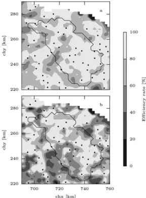
Precipitation threshold estimation
The threshold estimation analysis based on the existing sensor network showed a significant dif-ference between the two precipitation intensity thresholds (Fig. 7). While the efficiency rate for the
5 mm h–1threshold was over 80% for most of the
catchment, for a precipitation intensity threshold of 10 mm h–1the efficiency rate decreased and was for
large parts of the catchment between 40% and 60% (Fig. 7).
The catchment average efficiency rate changed for different rain gauge sensor network configura-tions and its range was similar to the analysis of the interpolation performance presented before. The catchment average efficiency rate was reason-ably high for all scenarios (right below 80% in the worst cases) and increased with increasing station density (Fig. 8). The efficiency rate reached a plateau for a density of 24 rain gauges per 1000 km2. For the higher threshold value
(10 mm h–1) the efficiency rate had an overall lower
average and larger range than for the lower thresh-old, but with a significant fraction of the grid cells presenting 100% efficiency.
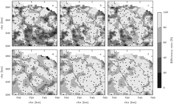
Finally, the efficiency rates of rain gauge network configurations with densities of eight and 24 rain gauges per 1000 km2, representing the
removal of eight rain gauges and the inclusion of 20 rain gauges respectively, was assessed (Fig. 9). The efficiency rate for the high precipitation inten-sity threshold was shown to deteriorate signifi-cantly when high-elevation stations are removed from the analysis, reaching levels as low as 20% for those areas. For the lower threshold efficiency this reduction was more moderate. However, the addition of 20 hypothetical stations produced an improvement of the efficiency rate in most areas of the catchment for both network configurations created with the different error indices. Efficiencies for the higher threshold are overall lower than for the lower threshold as well. For the lower precipi-tation intensity threshold, an area with significantly lower efficiencies was found close to the coordi-nates [720, 260] for the configuration obtained using theIPCCindex.
Discussion
The results obtained in this study indicate that the use of the existing precipitation monitoring network in the Thur catchment for spatial precipi-tation interpolation may produce significant errors, especially for high precipitation intensities (Figs 3 and 7). The heterogeneous rain gauge density con-centrates the highest errors in the areas with lower station densities which, such as the south-western edge of the catchment, also tend to show the highest average precipitation magnitudes (Fig. 2).
Fig. 7. Threshold estimation performance for the existing rain gauge network configuration for different precipitation intensity threshold levels. (a) Threshold of 5 mm h–1. (b) Threshold of
10 mm h–1. The individual rain gauges are represented as solid
squares. The coordinates are expressed in the CH1903 Swiss coordinate system.
Fig. 8. Catchment average precipitation intensity threshold estimation performance for an interpolation resolution of 36 km2and for
different rain gauge network configurations. (a) Estimation of the 10 mm h–1threshold for network configurations obtained by I RMSE.
(b) Estimation of the 10 mm h–1threshold for network configurations obtained by I
PCC. (c) Estimation of the 5 mm h–1threshold for
network configurations obtained by IRMSE. (d) Estimation of the 5 mm h–1threshold for network configurations obtained by IRMSE. The
box representing the existing configuration is shadowed.
Fig. 9. Precipitation intensity threshold estimation performance of two characteristic rain gauge network configurations for the different indicators and an interpolation resolution of 36 km2. (a) Estimation of the 10 mm h–1threshold after the removal of eight rain
gauges. (b) Estimation of the 10 mm h–1threshold after the placement of 20 rain gauges obtained by I
RMSE. (c) Estimation of the
10 mm h–1threshold after the placement of 20 rain gauges obtained by I
PCC. (d) Estimation of the 5 mm h–1threshold after the removal
of eight rain gauges. (e) Estimation of the 5 mm h–1threshold after the placement of 20 rain gauges obtained by I
RMSE. (f) Estimation
of the 5 mm h–1threshold after the placement of 20 rain gauges obtained by I
PCC. The existing rain gauge network is represented by
the solid squares, the stations removed by empty circles and the stations added by crosses. The coordinates are expressed in the CH1903 Swiss coordinate system.
However, when the interpolated precipitation mag-nitudes correspond to low precipitation intensities, the performance is satisfactory (over 80% effi-ciency for the estimating intensities of 5 mm h–1)
(Fig. 7).
Increasing the rain gauge density in the catch-ment, effectively reducing distances between rain gauges as well as establishing a more homogene-ous sensor distribution, significantly reduced pre-cipitation interpolation errors. A levelling off of the performance was seen when a density of 24 rain gauges per 1000 km2 (20 hypothetical stations
added) was achieved, which supports the results by Xuet al. (2013). This corresponded to a doubling of the rain gauge density from the existing sensor network configuration and a six-fold increase with respect to the minimum recommended density for mountainous areas (WMO 2008). Beyond this density value further interpolation error reductions were negligible. Looking at the threshold analysis, the significant number of grid cells showing 100% efficiency for the higher threshold were attributed to the fact that the frequency of such events in those locations is small, which may cause a bias in the efficiency range. In such circumstances the prob-ability of having perfect efficiency is much higher than for higher frequencies.
Reducing the rain gauge density in high eleva-tion areas of the catchment was found to have a strong effect on the performance of the interpola-tion. The lower rain gauge density combined with the high precipitation amounts and variability in these areas resulted in a strong increase of the interpolation error. The effect was also noticed in the catchment averages, which showed a much higher error increase rate than for the scenario involving increasing rain gauge densities. Overall, the availability of rain gauges in remote, high elevation areas was found to be more important for the correct estimation of spatial precipitation inten-sities, and more specifically for high intensity pre-cipitation thresholds than, for instance, a slight increase basin-wide station density. High precipi-tation intensities and amounts in high altitudes, combined with a high variability, make data gath-ering in these regions extremely important for rel-evant water management practices such as flood planning and management.
The similarity in the placement of hypothetical rain gauges by the different error indices could mainly be attributed to the fact that the areas with largest precipitation variability are the same as the areas with largest precipitation amounts.
Regarding the precipitation intensity estimation, the performance of the different network configu-rations for a threshold of 10 mm h–1was
consider-ably lower than for a threshold of 5 mm h–1. It
might be reasonable to assume that the efficiency of the rain gauge network for estimating higher precipitation intensities would be even lower, making the estimation of high precipitation inten-sities uncertain.
The different spatial resolutions used for the evaluation produced slightly different results. For a resolution of 4 km2the magnitude and variability
of interpolation errors were generally higher than for a resolution of 36 km2, which is in agreement
with the findings by MeteoSwiss (2013a). The per-formance differences were however found to be relatively small compared with the magnitude of the errors which is attributed to the fact that the small scale precipitation variability is smoothened out for both cases. However, the smoothening out of the small-scale variability had the side effect of missing relevant local, high-intensity events. While these results are not directly comparable to those from Goodrichet al. (1995) as the range evaluation resolutions they tested was significantly larger, the same general trend was found.
The results presented here need to be viewed with caution as the analysis was performed using an estimate of the real precipitation. As previously mentioned, the data used for this purpose present a general small positive bias as well as a tendency to overestimate low intensities and underestimate high intensities. In this particular setting, however, the radar beam shielding by the mountain ranges does not appear to be a main concern. Overall, the validity of the present study is dependent on the errors of the underlying data used and should not be used as an exact measure of rain gauge network performance for monitoring spatial pre-cipitation variability, but rather as an indicative estimation.
Conclusions
The existing heterogeneous monitoring sensor network performed well for low to normal precipi-tation intensities (up to 10 mm h–1). In the areas
where low rain gauge densities are combined with high precipitation intensities the efficiency of the sensor network decreases significantly. This sug-gests that the current sensor network is appropriate for monitoring the area but with a significant prob-ability of missing rare and localised events.
An increase in the rain gauge density consider-ably improves the performance of the sensor network for all error indices tested. A levelling off of the interpolation errors is found after a rain gauge density of approximately 24 rain gauges per 1000 km2 is reached. Beyond this station density
value the contribution of additional stations is negligible
The effects of localised rain gauge station density reduction at high elevation areas was shown to produce a significant decrease in the ability to estimate distributed precipitation where both the magnitudes and variability were highest. The significant efficiency decrease of the rain gauge network for this scenario emphasises the importance of carefully dimensioning pluviometric sensor networks.
Finally, future work in two main directions can be motivated by the results of this study. One is extending the analysis period to include more extreme precipitation events combined with a more general study including hydrological modelling and cost–benefit estimations of the analysed high-precipitation events. The other is alternative place-ment strategies for deploying additional rain gauges, including several metrics such as variance over time and space, but also factors such as acces-sibility of a station should be considered. The latter would include questions such as whether it might be more useful to run two relatively inexpensive stations in easily accessible, low-elevation loca-tions or one expensive station at a more difficult-to-access high-elevation location.
Marc Girons Lopez, Department of Earth Sciences, Uppsala University, Villavägen 16, 752 36 Uppsala, Sweden E-mail:[email protected]
Hjalmar Wennerström, Lars-Åke Nordén, Department of Information Technology, Uppsala University, PO Box 337, 751 05 Uppsala, Sweden
E-mail: [email protected], lars-ake.norden@ it.uu.se
Jan Seibert, Department of Geography, University of Zurich, Winterthurerstrasse 190, CH-8057 Zurich, Switzerland E-mail:[email protected]
References
Anctil, F., Lauzon, N., Andréassian, V., Oudin, L. and Perrin, C., 2006. Improvement of rainfall-runoff forecasts through mean areal rainfall optimization. Journal of Hydrology, 328 (3–4), 717–725. doi: 10.1016/ j.jhydrol.2006.01.016
Andréassian, V., Perrin, C., Michel, C., Usart-Sanchez, C. and Lavabre, J., 2001. Impact of imperfect rainfall
knowledge on the efficiency and the parameters of water-shed models.Journal of Hydrology, 250 (1–4), 206–223. doi: 10.1016/S0022-1694(01)00437-1
Balme, M., Vischel, T., Level, T., Peugeot, C. and Galle, S., 2006. Assessing the water balance in the Sahel: impact of small scale rainfall variability on runoff. Part 1: Rainfall variability analysis. Journal of Hydrology, 331 (1–2), 336–348. doi: 10.1016/j.jhydrol.2006.05.020
Bárdossy, A. and Das, T., 2008. Influence of rainfall obser-vation network on model calibration and application.
Hydrological and Earth System Sciences, 12 (1), 77–89. doi: 10.5194/hess-12-77-2008
Biggs, E.M. and Atkinson, P.M., 2011. A comparison of gauge and radar precipitation data for simulating an extreme hydrological event in the Severn Uplands, UK.
Hydrological Processes, 25 (5), 795–810. doi: 10.1002/ hyp.7869
Chow, V. Te, Maidment, D.R. and Mays, L.W., 1988.
Applied Hydrology. McGraw-Hill Series in Water Resources and Environmental Engineering. McGraw-Hill, New York. ISBN 0-07-010810-2.
Clark, M.P. and Slater, A.G., 2006. Probabilistic quantitative precipitation estimation in complex terrain.Journal of Hydrometeorology, 7 (1), 3–22. doi: 10.1175/JHM474.1 FOEN, 2013. Hochwasserwahrscheinlichkeiten
(Jah-reshochwasser) DB-Nr. 136 Thur-Andelfingen, 1 p. Frei, C. and Schär, C., 1998. A precipitation climatology of
the alps from high-resolution rain-gauge observations.
International Journal of Climatology, 18, 873–900. doi: 10.1002/(SICI)1097-0088(19980630)18:8< 873::AID-JOC255>3.0.CO;2-9
Frei, C., Schöll, R., Fukutome, S., Schmidli, J. and Vidale, P.L., 2006. Future change of precipitation extremes in Europe: intercomparison of scenarios from regional climate models.Journal of Geophysical Research, 111, 1–22. doi: 10.1029/2005JD005965
FSO, 2013. Regional portraits 2013: Communes, 4878 p.
Goodrich, D.C., Faurès, J.-M., Woolhiser, D.A., Lane, L.J. and Sorooshian, S., 1995. Measurement and analysis of small-scale convective storm rainfall variability.Journal of Hydrology, 173 (1–4), 283–308. doi: 10.1016/0022-1694(95)02703-R
Haberlandt, U., 2011. Interpolation of precipitation for flood modelling. In: Schumann, A.H. (ed.),Flood Risk Assess-ment and ManageAssess-ment. Springer, Berlin, 35–52. doi: 10.1007/978-90-481-9917-4_3
Jones, J.A.A., 1997. Global Hydrology. Processes, Resources and Environmental management. Pearson Education Ltd, Harlow, UK.
Joss, J., Schädler, B., Galli, G., Cavalli, R., Boscacci, M., Held, E., Della Bruna, G., Kappenberger, G., Nespor, V. and Spiess, R., 1997. Operational Use of Radar for Precipitation Measurements in Switzerland. Federal Office of Meteorology and Climatology (MeteoSwiss), Zurich.
McMillan, H., Krueger, T. and Freer, J., 2012. Benchmark-ing observational uncertainties for hydrology: rainfall, river discharge and water quality. Hydrological Pro-cesses, 26 (26), 4078–4111. doi: 10.1002/hyp.9384 Messer, H., Zinevich, A. and Alpert, P., 2006. Environmental
monitoring by wireless communication networks.
MeteoSwiss, 2013a. Daily Precipitation (final analysis): RhiresD. (August). Federal Office of Meteorology and Climatology (MeteoSwiss), Zurich. 4 p.
MeteoSwiss, 2013b.Hourly Precipitation (Experimental): RdisaggH. Federal Office of Meteorology and Climatol-ogy (MeteoSwiss), Zurich. 4 p.
MeteoSwiss, 2013c.Projet Rad4Alp: un réseau moderne de radars pour les Alpes suisses. Federal Office of Meteor-ology and ClimatMeteor-ology (MeteoSwiss), Zurich. MeteoSwiss, 2014a. Normes climatologiques St. Gallen.
Période de référence 1981–2010. Federal Office of Meteorology and Climatology (MeteoSwiss), Zurich. 2 p.
MeteoSwiss, 2014b. Stations of the manual precipitation monitoring network of MeteoSwiss. Federal Office of Meteorology and Climatology (MeteoSwiss), Zurich. 7 p.
Peck, E.L. and Brown, M.J., 1962. An approach to the devel-opment of isohyetal maps for mountainous areas.
Journal of Geophysical Research, 67 (2), 681–694. doi: 10.1029/JZ067i002p00681
PEER, 2010. River Thur – Hydrological observatory description. Partnership for European Environmental Research (PEER).
Price, K., Purucker, S.T., Kraemer, S.R., Babendreier, J.E. and Knightes D., 2013. Comparison of radar and gauge precipitation data in watershed models across varying spatial and temporal scales.Hydrological Processes, 28 (9), 3505–3520. doi: 10.1002/hyp.9890
Savvidou, K., Michaelides, S., Nicolaides, K.A. and Constantinides, P., 2009. Presentation and preliminary evaluation of the operational Early Warning System in Cyprus.Natural Hazards and Earth System Science, 9 (4), 1213–1219. doi: 10.5194/nhess-9-1213-2009 Schuurmans, J.M. and Bierkens, M.F.P., 2007. Effect of
spatial distribution of daily rainfall on interior catchment response of a distributed hydrological model. Hydrologi-cal and Earth System Sciences, 11 (1995), 677–693. doi: 10.5194/hess-11-677-2007
Schwarb, M., Daly, C., Frei, C. and Schär, C., 2001. Mean annual and seasonal precipitation in the European Alps 1971–1990.Hydrological Atlas of Switzerland. Federal Office for the Environment FOEN, Bern.
Shepard, D., 1968. A two-dimensional interpolation function for irregularly-spaced data. In:Proceedings of the 1968 23rd ACM national conference. ACM Press, New York. 517–524. doi: 10.1145/800186.810616
Suter, S., Konzelmann, C., Mühlhäuser, C., Begert, M. and Heimo, A., 2006. SwissMetNet – the new automatic meteorological network of Switzerland: transition from old to new network, data management and first results. Federal Office of Meteorology and Climatology (MeteoSwiss), Zurich.
Tilford, K.A., Sene, K. and Collier, C.G., 2003.Flood Fore-casting – Rainfall Measurement and ForeFore-casting. Envi-ronment Agency, Bristol.
UN, 2006. Global Survey of Early Warning Systems. An assessment of capacities, gaps and opportunities towards building a comprehensive global early warning system for all natural hazards. United Nations, Geneva. Vogl, S., Laux, P., Qiu, W., Mao, G. and Kunstmann, H.,
2012. Copula-based assimilation of radar and gauge information to derive bias corrected precipitation fields.
Hydrology and Earth System Sciences Discussions, 9 (1), 937–982. doi: 10.1145/800186.810616
Weber, D. and Englund, E., 1992. Evaluation and compari-son of spatial interpolators.Mathematical Geology, 24 (4), 381–391. doi: 10.1007/BF00891270
WMO, 2008. Guide to Hydrological Practices. Volume I: Hydrology – From Measurement to Hydrological Infor-mation, 6th edition. World Meteorological Organization, Geneva.
WMO, 2011.Manual on Flood Forecasting and Warning. World Meteorological Organization, Geneva.
Wood, S.J., Jones, D.A. and Moore, R.J., 2000. Accuracy of rainfall measurement for scales of hydrological interest.
Hydrology and Earth System Sciences, 4 (4), 531–543. doi: 10.5194/hess-4-531-2000
Xu, H., Xu, C.-Y., Chen, H., Zhang, Z. and Li, L., 2013. Assessing the influence of rain gauge density and distri-bution on hydrological model performance in a humid region of China.Journal of Hydrology, 505, 1–12. doi: 10.1016/j.jhydrol.2013.09.004
Manuscript received 2 Feb., 2014, revised and accepted 16 Dec., 2014