Improving the Classification of Multiple Disorders with Problem Decomposition

Improving the Classification of Multiple Disorders

with Problem Decomposition

Radwan E. Abdel-Aal

, Mona R. E. Abdel-Halim

, and Safa Abdel-Aal

1_{Computer Engineering Department, King Fahd University of Petroleum and Minerals,}

Dhahran, Saudi Arabia

2_{Dermatology Department, Faculty of Medicine, Cairo University, Cairo, Egypt} 3_{Derriford Hospital, Plymouth, Devonshire, UK}

Address for corresponding author and reprints:

Dr. R. E. Abdel-Aal

P. O. Box 1759

KFUPM

Dhahran 31261

Saudi Arabia

e-mail:

[email protected]

Phone: +966 3 860 4320

Fax: +966 3 860 4281

Abstract

Differential diagnosis of multiple disorders is a challenging problem in clinical medicine. According to the divide-and-conquer principle, this problem can be handled more effectively through decomposing it into a number of simpler sub-problems, each solved separately. We demonstrate the advantages of this approach using abductive network classifiers on the 6-class standard dermatology dataset. Three problem decomposition scenarios are investigated, including class decomposition and two hierarchical approaches based on clinical practice and class separability properties. Two-stage classification schemes based on hierarchical decomposition boost the classification accuracy from 91% for the single-classifier monolithic approach to 99%, matching the theoretical upper limit reported in the literature for the accuracy of classifying the dataset. Such models are also simpler, achieving up to 47% reduction in the number of input variables required, thus reducing the cost and improving the convenience of performing the medical diagnostic tests required. Automatic selection of only relevant inputs by the simpler abductive network models synthesized provides greater insight into the diagnosis problem and the diagnostic value of various disease markers. The problem decomposition approach helps plan more efficient diagnostic tests and provides improved support for the decision making process. Findings are compared with established guidelines of clinical practice, results of data analysis, and outcomes of previous informatics-based studies on the dataset.

Keywords:

Classifiers, Abductive Networks, Neural Networks, Problem Decomposition, Divide and Conquer, Classification Accuracy, Data Reduction, Modular Networks, Medical Diagnosis, Multiple Disorders, Dermatology.

1. Introduction

Differential diagnosis among a group of disorders having similar symptoms and signs poses a challenging problem in clinical medicine. According to the divide-and-conquer principle, classification of multiple disorders can be performed more efficiently through problem decomposition [1], particularly when various diagnoses are independent and the causes underlying them do not interact. Instead of tackling the whole complex problem at once, the problem is divided into a number of simpler sub-problems, each of which is solved separately. Problem decomposition also helps the user better understand the diagnostic situation and provide required interpretations and justifications [1]. The hierarchical nature of this approach makes the classification easier to understand and helps guide the diagnosis process [2]. Resulting partial diagnoses could also prove useful in explaining findings and deciding upon further diagnostic tests to be performed next. Early diagnostic programs, e.g. [3], have applied pattern sorting methods to group disorders based on similarity of symptoms. The hierarchical approach to diagnosis has also been used to implement several medical expert systems [4].

Machine learning classification techniques are being increasingly used for decision-making support in medicine. Such techniques include Bayesian and nearest-neighbor classifiers, rule induction methods, decision trees, fuzzy logic, artificial neural networks, and abductive networks [5] based on the group method of data handling (GMDH) algorithm [6]. Compared to neural networks, abductive networks allow easier model development and provide more transparency and greater insight into the modeled phenomena, which are important advantages in medicine. Medical applications of GMDH-based techniques include modeling obesity [7], analysis of school health surveys [8], drug detection from EEG measurements [9], medical image recognition [10], and screening for delayed gastric emptying [11]. Neural networks have been used to solve many multiclass classification problems directly using a single network. Examples of such applications include categorizing arrhythmia types from ECG signals [12], diagnosing eye diseases [13], classifying the severity of diabetic retinopathy

[14], discriminating between dyslexic subtypes [15], classifying various types of aphasia [16], classifying sleep stages from EEG signals [17], differential diagnosis of eleven interstitial lung diseases [18], differential diagnosis among different types of dementia [19], and discriminating between pancreatic ductal adenocarcinoma and mass-forming pancreatitis based on CT findings [20].

Training a single network to solve a complex multiclass classification problem may suffer from strong interferences that slow down convergence and degrade generalization [21]. The divide-and-conquer approach has been proposed to improve the performance and realization of neural network solutions to real life problems through problem decomposition. Instead of tackling the whole complex problem in one go, the problem is divided into a number of simpler, more manageable sub-problems, each of which can be solved by a network module. The resulting modules are simpler than a single (monolithic) network that attempts to solve the problem as a whole, and therefore would generalize better, thus improving classification performance. Such modules would also require fewer inputs and train faster. Various modules can be trained in parallel, which further reduces training time. They would also be easier to realize physically as VLSI circuits where practical limitations exist on the number of connections associated with a node [22]. Resulting smaller modular networks reduce the requirement on the training sample size, which is useful in handling high-dimensionality data often encountered in medicine.

A number of approaches exist for decomposing a complex problem into a set of simpler ones. In the manual approach, decomposition is performed by the designer prior to training, based on prior knowledge of the classification problem. Class decomposition, e.g. [23], is a straight forward approach, where a K-class classifier is replaced by K two-class modules, each trained to recognize one class from its complement. Hierarchical approaches, e.g. [24], perform classification in a number of sequential stages. Techniques have also been described for performing the decomposition automatically during training without requiring prior knowledge of the problem, e.g. [25]. Using

network committees (ensembles) is another related modular approach for improving classification accuracy. With this approach, a number of independent classifiers, each trained to solve the whole problem from a different perspective, are used simultaneously and their outputs combined to produce the final classifier output. Ensembles of abductive networks trained on different subsets of the training set have proved useful in improving the classification accuracy of a number of standard medical datasets including the dermatology dataset [26].

Chi and Jabri [24] adopted a two-stage problem decomposition approach using three neural networks to classify intracardiac electrograms (IECGs) rhythms into four classes for identifying Supraventricular and Ventricular Arrhythmias. Compared a monolithic solution that uses a single more complex network, problem decomposition improved the classification accuracy from 89.3% to 96.2%. Wen and Ozdamar [23] used a scheme of modular neural networks based on class decomposition to classify auditory brainstem response, improving the rate of correct classification from 76.6% to 82.4%. The divide-and-conquer approach was used to build a system of multimodule contextual neural networks for the automatic identification of abdominal organs from computed tomography (CT) image series, where each module focuses on extracting the regions of one organ [27]. Ohno-Machado and Musen [2] developed a hierarchical system of neural networks for diagnosing thyroid diseases through grouping them into four superclasses. The system trained faster, required fewer inputs, and generally proved more accurate compared to the monolithic alternative. West and West [21] employed a two-stage hierarchical neural network to classify the six-class of the dermatology dataset [28] with an accuracy of 98.4% which approaches the 98.6% maximum theoretical limit envisaged for the classification accuracy. The network combines a multiplayer perceptron first stage with a mixture of expert second stage designed to learn the particularly difficult subtask of discriminating between two overlapping classes. A previous investigation on abductive network classifiers has shown that problem decomposition improves classification accuracy of

waveform patterns and makes the classifiers more tolerant to model simplification and reductions in the training set size compared to monolithic solutions [29].

This paper investigates improvements in classifying the multiclass dermatology dataset [28] with abductive network classifiers using various scenarios of problem decomposition. The dataset consists of 358 records, each having 34 input features, diagnosed into six diseases (classes). Results are compared with those of conventional monolithic alternatives and other problem decomposition approaches reported in the literature. Section 2 gives a brief introduction to the GMDH algorithm, the abductive network modeling tool used, and the problem decomposition approaches adopted. Section 3 gives a brief outline of the dermatology dataset used in the investigation. Section 4 presents the results obtained and compares findings with those reported in the literature. In addition to improving classification accuracy, problem decomposition offers simpler classifiers that use fewer disease markers, thus reducing the cost and improving the convenience of performing medical diagnostic tests. Information gained on the relevance of various input features to the diagnosis of various types of dermatology disorders are compared with clinical experience and with findings from previous studies. Conclusions are made and suggestions given for future work in Section 5.

2. Methods

2.1 GMDH and AIM Abductive Networks

AIM (abductory inductive mechanism) [30] is a supervised inductive machine learning tool for automatically synthesizing abductive network models from a database of inputs and outputs representing a training set of solved examples. As a GMDH algorithm, the tool can automatically synthesize adequate models that embody the inherent structure of complex and highly nonlinear systems. Automation of model synthesis not only lessens the burden on the analyst but also safeguards the model generated against influence by human biases and misjudgments. The GMDH approach is a

degree polynomial model in effective predictors. The process is 'evolutionary' in nature, using initially simple (myopic) regression relationships to derive more accurate representations in the next iteration. To prevent exponential growth and limit model complexity, the algorithm selects only relationships having good predicting powers within each phase. Iteration is stopped when the new generation regression equations start to have poorer prediction performance than those of the previous generation, at which point the model starts to become overspecialized and therefore unlikely to perform well with new data. The algorithm has three main elements: representation, selection, and stopping. It applies abduction heuristics for making decisions concerning some or all of these three aspects.

To illustrate these steps for the classical GMDH approach, consider an estimation data base of

ne observations (rows) and m+1 columns for m independent variables (x1, x2, ..., xm) and one dependent

variable y. In the first iteration we assume that our predictors are the actual input variables. The initial

rough prediction equations are derived by taking each pair of input variables (xi, xj ; i,j = 1,2,...,m)

together with the output y and computing the quadratic regression polynomial [6]:

y = A + Bxi + C xj + D xi2+ E xj2 + F xi xj (1)

Each of the resulting m(m-1)/2 polynomials is evaluated using data for the pair of x variables used to

generate it, thus producing new estimation variables (z1, z2, ..., zm(m-1)/2) which would be expected to

describe y better than the original variables. The resulting z variables are screened according to some

selection criterion and only those having good predicting power are kept. The original GMDH algorithm employs an additional and independent selection set of ns observations for this purpose and

uses the regularity selection criterion based on the root mean squared error rk over that dataset, where:

1)/2 m 1,2,...,m( k ; y ) z (y r s s n 1 2 n 1 2 k 2 k =

∑

∑

the minimum value, rmin, obtained for rk is also saved. The selected z variables represent a new

higher-level variables. At each iteration, rmin is compared with its previous value and the process is continued

as long as rmin decreases or until a given model complexity is reached. An increasing rmin is an

indication of the model becoming overly complex, thus overfitting the estimation data and performing poorly on the new selection data. Keeping model complexity checked is an important aspect of GMDH-based algorithms, which keep an eye on the final objective of constructing the model, i.e. using it with new data previously unseen during training. The best model for this purpose is that providing the shortest description for the data available [31]. Computationally, the resulting GMDH model can be seen as a layered network of partial quadratic descriptor polynomials, each layer representing the results of an iteration.

A number of GMDH methods have been proposed which operate on the whole training dataset thus eliminating the need for a dedicated selection set. The adaptive learning network (ALN) approach, AIM being an example, uses the predicted squared error (PSE) criterion [31] for selection and stopping to avoid model overfitting, thus solving the problem of determining when to stop training in neural networks. The criterion minimizes the expected squared error that would be obtained when the network is used for predicting new data. AIM expresses the PSE as:

2 ) 2 ( K N _p CPM FSE PSE = +

σ

where FSE is the fitting squared error on the training data, CPM is a complexity penalty multiplier

selected by the user, K is the number of model coefficients, N is the number of samples in the training

set, and is a prior estimate for the variance of the error obtained with the unknown model. This estimate does not depend on the model being evaluated and is usually taken as half the variance of the dependent variable y [31]. As the model becomes more complex relative to the size of the training set,

the second term increases linearly while the first term decreases. PSE goes through a minimum at the

optimum model size that strikes a balance between accuracy and simplicity (exactness and generality). The user may optionally control this trade-off using the CPM parameter. Larger values than the default

2

p σ

value of 1 lead to simpler models that are less accurate but may generalize well with previously unseen data, while lower values produce more complex networks that may overfit the training data and degrade actual prediction performance.

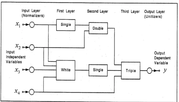
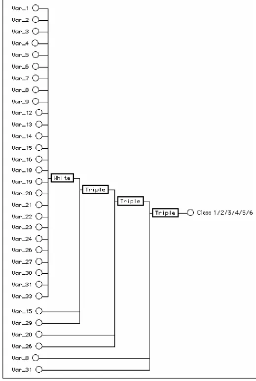
AIM builds networks consisting of various types of polynomial functional elements. The network size, element types, connectivity, and coefficients for the optimum model are automatically determined using well-proven optimization criteria, thus reducing the need for user intervention compared to neural networks. This simplifies model development and considerably reduces the learning/development time and effort. The models take the form of layered feed-forward abductive networks of functional elements (nodes) [30], see Fig. 1. Elements in the first layer operate on various combinations of the independent input variables (x's) and the element in the final layer produces the

predicted output for the dependent variable y. In addition to the main layers of the network, an input

layer of normalizers convert the input variables into an internal representation as Z scores with zero

mean and unity variance, and an output unitizer unit restores the results to the original problem space. AIM supports the following main functional elements:

(i) A white element which consists of a constant plus the linear weighted sum of all outputs of the previous layer, i.e.

"White" Output = w₀ + w₁x₁+ w₂x₂ + w₃x_{3 + .... +} w_nx _{n (4)}

where x₁, x₂,..., x_nare the inputs to the element and w₀, w₁, ..., w_n are the element weights.

(ii) Single, double, and triple elements which implement a third-degree polynomial expression with all possible cross-terms for one, two, and three inputs respectively; for example,

"Double" Output = w_{0 + w1}x_{1 + w2}x_{2 + w3}x₁2 + w₄x₂2 + w₅x₁x_{2 + w6}x₁3 + w₇x₂3 (5)

2.2 Classification with Problem Decomposition

Classification with problem decomposition entails dividing the decision domain into a number of smaller subtasks that are more easily handled using dedicated classifiers. Fig. 2 sketches a straight

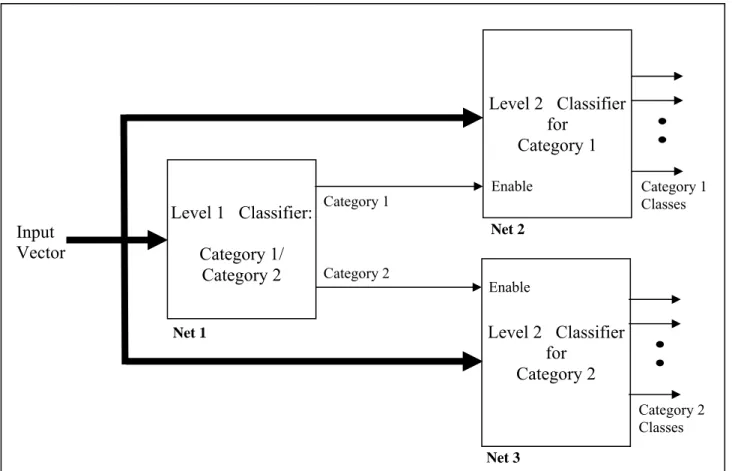
forward, non-hierarchical arrangement of solving a K-class classification problem using class decomposition. Instead of using a single complex classifier to solve the problem, K binary classifier modules are used in parallel, each trained to identify only one class from its complement. Individual modules handle simpler tasks and therefore are expected to be simpler than a single (monolithic) classifier tackling the entire problem. Since class classifiers can be trained and interrogated in parallel, faster training and classification is expected. Using classification techniques that indicate the input features selected by the classifier, e.g. decision trees and GMDH based methods, this approach reveals disease markers that are important for differentially diagnosing each class from the remaining classes. One limitation of this approach is the gross imbalance in the composition of training sets for individual modules. For example, if all K classes are equally represented in the dataset, the ratio of training records pertaining to the class of interest to the remaining classes is 1/(K-1). For a large number of classes, this ratio would be low, which slows down training and degrades classification performance [32]. Multi-stage hierarchical problem decomposition attempts to overcome this limitation. Fig. 3 shows a two-stage arrangement where the classes are grouped into two categories (superclasses), each containing a number of classes. The correct superclass is first determined by the classifier in the first stage, and then the appropriate classifier in the second stage is used to determine the class within that superclass. Although classifier modules can still be trained in parallel, actual classification is sequential. One challenging aspect of this approach is splitting the classification problem into two or more subproblems which are at least partially independent. Wu [1] applied the symptom decomposition method as a systematic approach to solve partially decomposable medical diagnostic problems. In this paper we investigate two heuristic approaches to problem decomposition for the six-class standard dermatology dataset: one based on clinical diagnostic practice and the other based on class separability properties reported in the literature.

3. Material

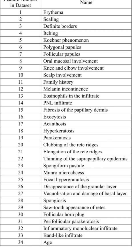
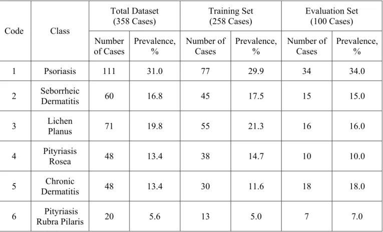
The dermatology standard medical diagnosis dataset from the UCI Machine Learning Repository [33] was used for this study. This multiclass dataset [28] has been used for the differential diagnosis of Erythemato-Squamous diseases. It consists of 366 records, each having 34 attributes. Table 1 lists the names or brief descriptions of the input attributes for the dataset. The attributes include age and 11 other clinical attributes (attributes numbered 1-11), and 22 histopathological features (attributes numbered 12-33) determined by the analysis of skin samples under the microscope. Each attribute other than age and family history was given a score in the range 0 to 3, where 0 indicates the feature being absent, 3 indicates the largest amount possible, and 1, 2 indicate intermediate values. The feature number used in the table is the column number for the feature in the dataset. The class output variable (variable 35 in the dataset) is an integer code ranging from 1 to 6 that indicates the following six possible diseases: psoriasis, seborrheic dermatitis, lichen planus, pityriasis rosea, chronic dermatitis, and pityriasis rubra pilaris, respectively. Eight records in the original dataset had the age attribute missing, and these were excluded, leaving 358 records for use in this study. The 358 records were randomly split into a training set and an evaluation set of 258 and 100 records, respectively. Table 2 gives details of the distribution of the six disease classes in the total, training, and evaluation datasets as determined by the class variable. Using single classifiers based on the C4.5 decision-tree induction algorithm, a classification accuracy of 89.1% was obtained with a five-fold cross validation procedure [34]. Classification accuracies of 92.25% and 86.15% were achieved on this dataset with feed forward back propagation neural networks and conventional radial basis function neural networks, respectively [35].

4. Results

4.1Monolithic Models

Monolithic AIM abductive models of various complexities were developed to solve the whole classification problem at once. Model inputs comprised the full set of 34 input features of the data set (Table 1), and the model had a single multi-valued output with the values 1, 2, 3, 4, 5, and 6 representing the six disease classes as given in Table 2. Each model was trained using the full training set of 258 records and evaluated using the evaluation set consisting of the remaining 100 records. Categorical classifier output was derived from the linear model output by rounding through simple crossing of threshold levels located half-way between adjacent class values. For example, class 1 is represented by: output < 1.5, class 3 is represented by: 2.5 ≤ output < 3.5, while class 6 is represented by: 5.5 ≤ output. Various models of different complexity were synthesized using different CPM values, e.g. CPM = 1 (default model), CPM = 0.5 (more complex model), and CPM = 2 (less complex model). The model with CPM = 0.5 gave the highest value of 91% for the classification accuracy. Fig. 4 shows the structure of this 4-layer model. Only 27 out of the 34 input features are automatically selected by the learning algorithm as model inputs. The numbers indicated at the model input in Fig. 4 refer to the feature numbers listed in Table 1. The seven features discarded by the model are those numbered 10, 11, 17, 25, 28, 32, and 34. A data reduction procedure carried out on this dermatology dataset using stepwise discriminant analysis has identified nine input features {1,3,9,10,17,23,27,30,34} that do not contribute significantly to the discrimination of the six classes [21]. These included features 10, 17, and 34 discarded by the AIM model described above. Table 3 (a) shows the confusion matrix obtained when this monolithic model was evaluated on the 100 cases of the evaluation set. The table shows the overall percentage classification accuracy in the bottom right cell. Poorest performance is associated with the identification of class 6, followed by classes 2 and 4 respectively. As indicated in Table 2, class 6 is thinly represented in the data set at only 5.6%, and therefore the number of training examples

for this class may not be sufficient for adequate learning. Exploratory data analysis performed by West and West [21] on the dermatology dataset using self organizing maps (SOMs) revealed that classes {1,3,5,6} form distinct clusters that do not overlap in the SOM map, and therefore should be identified with a higher degree of accuracy compared to classes 2 and 4. They have shown that classes 2 and 4 overlap on the SOM map at five cases in the total dataset of 358 cases due to inconsistency or wrong diagnosis, concluding that sets an upper limit of 98.6% for the classification accuracy for the dermatology dataset. It is expected that classifier schemes employing problem decomposition could improve on the classification accuracy of the complex monolithic model through better learning and identification of classes 2, 4, and 6.

4.2Class Decomposition Approach

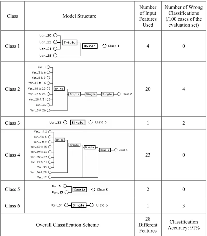
In line with the class decomposition scheme depicted in Fig. 2, six abductive models were developed, each trained to identify only one class. Referring to Table 2, the model for class 6, for example, was trained on 258 cases of which 13 cases are class 6 and 245 cases are not class 6, and therefore the ratio between the in-class and out-of-class cases is only 0.05. The model was evaluated on 100 cases of which 7 cases are class 6 and 93 cases are not class 6. In the training set, the class output is assigned the value of 2 for the in-class cases and the value of 1 for the out-of-class cases. Table 4 shows the structure and performance of the six models synthesized at the default model complexity (CPM = 1). Overall classification accuracy is 91%, which is the same as the best monolithic model of Fig. 4. Table 3 (b) shows the confusion matrix obtained when the six class decomposition models were evaluated on the evaluation set. As expected, the modular classifiers are generally simpler than the monolithic model. The most complex models correspond to classes 2 and 4, which proved to be the most difficult classes to classify [21]. Among themselves, the six models use 28 different input features. The six features discarded are those numbered 10, 11, 24, 30, 32, and 34. Four of these features {10,11,32,34} were also discarded by the monolithic model described in Section

4.1 above, and three {10,30,34} are among the nine features discarded by the data reduction procedure described in [21].

The unique property of automatic selection of only the most relevant input features by abductive network models gives useful insight into the diagnostic value of the various features in the dataset. For example, Table 4 shows that the model for class 1 (Psoriasis) uses four features: 20 (Clubbing of the rete ridges), 22 (Thinning of the suprapapillary epidermis), 28 (Spongiosis), and 31 (Perifollicular parakeratosis) and achieves 100% classification accuracy for this class. It is clinically established that histopathologic features of Psoriasis vary according to the stage of development of the lesion. Spongiosis is very mild and is usually seen only in the very early lesion. The fully developed psoriatic plaque is characterized by (a) acanthosis with regular elongation of the rete ridges with thickening in their lower portions (clubbing), (b) thinning of the suprapapillary epidermis with the occasional presence of small spongioform pustules of Kogoj, (c) pallor of the upper layers of the epidermis, (d) diminished or absent granular cell layer, (e) confluent parakeratosis, (f) presence of Munro microabscesses, (g) elongation and edema of the dermal papillae, and (h) dilated tortuous capillaries [36, 37]. This suggests that features 21 (Elongation of rete ridges), 23 (Spongioform pustules), 24 (Munro microabcesses), and 26 (Absent granular cell layer) should also contribute to the model. With the model already giving 100% classification accuracy without any of these features, the diagnostic value of these features in relation to the Psoriasis disorder appears to be poor for the dataset used. Class 3 disorder (Lichen Planus) can be diagnosed using only input feature number 33 (Band-like infiltrate). Inspection of the full data set revealed that the value of this feature is ≥ 2 for class 3 cases and is 0 for nearly all other cases. This feature is clinically recognized as a characteristic histopathological marker for this disorder, together with Damage to the basal cell layer (feature 27) and Saw-tooth appearance of retes (feature 29) [36]. Analysis of the dataset showed strong correlation between feature 33 selected by the model and the other two features, with the Pearson correlation

coefficients being 0.94 and 0.93 with features 27 and 29, respectively. Simple models in Table 4 allow the derivation of manageable analytical expressions that directly relate the classification output to the feature inputs. The model relationship is obtained through symbolic substitution of the equations determined by the learning algorithm for the various functional elements of the model. For example, substituting for the equations obtained for the normalizer, unitizer, and “Single” functional elements of the model for class 3, the class output can be determined from only the value of feature 33 (Var_33)

using the following relationships:

2 3

1 1.16667 _ 33 + 1.5 ( _ 33) 0.3333 ( _ 33) ,

y = − V ar V ar − V ar

Class = 3 if y ≥ 1.5 (6)

The model for Class 5 (Chronic Dermatitis) uses only two features: 5 (Koebner phenomenon) and 15 (Fibrosis of the papillary dermis) and achieves 100% classification accuracy for this class. Inspection of the data revealed that the value of feature 15 is ≥ 1 for class 5 and is 0 for nearly all other cases. Clinical experience confirms that Papillary dermal fibrosis (feature 15) is a justified feature for diagnosing chronic dermatitis and discriminating it from the remaining disorders. Class 6 disorder (Pityriasis Rubra Pilaris) can be diagnosed using only feature number 31 (Perifollicular parakeratosis). Inspection of the data revealed that the value of this feature is ≥ 1 for class 6 and is 0 for nearly all other cases. The localization of parakeratosis to perifollicular shoulders is often seen in the follicular keratotic lesions of the disorder, and is usually associated with dilated infundibulae filled with orthokeratotic horny plug [37]

In addition to comparing the results of class decomposition models given in Table 4 with knowledge gained from clinical practice, we compared the results with those derived from informatics perspectives. Valdes-Perez, Pericliev, and Pereira [38] have derived concise, intelligible, and approximate profiles for each class of the dermatology dataset. Each class profile consists of a minimized list of features annotated with how these features contrast the class from other classes.

Fidelis, Lopes, and Freitas [39] have used genetic algorithms (GA) to derive six comprehensive classification rules that describe the six dermatology classes, each maximizing a fitness function defined as the product of sensitivity and specificity for the class. Rules were derived using a training set consisting of 2/3 of the available records and tested on the remaining 1/3 of the records. Table 5 compares the features selected by the class decomposition approach with those derived by the approximate profiling and the classification rule approaches for each class. The table also lists the values of the fitness function (on a scale of 0 to 1) for each class for the latter approach. In all three approaches, identifying classes 2 and 4 represents the most difficult problem, as indicated by the large number of features required and the lowest values for the fitness function for those two classes. For example, approximate profiling suggests that each of classes 1, 3, 5, and 6 can be identified with a single feature while classes 2 and 4 require 5 and 3 features, respectively. Moreover, the three features used to identify class 4 are a subset of the five features used to identify class 2. This suggests that the group of classes {1,3,5,6} are more separable than the group {2,4}. Such observations agree with conclusions made by West and West [21]. All three approaches unanimously agree on feature 33 (Band-like infiltrate) as the sole predictor for class 3 (Lichen Planus). They also select feature 15 (Fibrosis of the papillary dermis) as a predictor for class 5 (Chronic Dermatitis). Approximate profiling is the only approach that made use of the feature 34 (Age), which is used as a sole predictor for class 6 (Pityriasis Rubra Pilaris) as opposed to feature 31 (Perifollicular parakeratosis) selected by class decomposition for this purpose. With the class output being 1 for class 6 and 0 otherwise, analysis of the full dataset reveals that the Pearson correlation coefficient between the class output and features 34 and 31 are –0.42 and 0.95, respectively, suggesting that feature 31 would be a better predictor for class 6.

4.3Hierarchical Problem Decomposition Approach

As shown by the results above, class decomposition did not improve classification performance beyond that of the best monolithic model, mainly because of the imbalance between the number of in-class and out-of-in-class cases during training of individual models. To overcome this limitation, we employed two-stage hierarchical problem decomposition of the type shown in Fig. 3. In the first stage, a classifier sorts the population into one of two categories (superclasses), which is then sorted into individual classes by the appropriate classifier in the second stage. If the class subsets for the two categories are {2,5} and {1,3,4,6}, then the category classifier in the first stage would have an in-class/out-of-class ratio of 0.41 for its training set (refer to relevant class distribution data in Table 2). In the second stage, the classifier handling the second category would be trained to identify class 6 with an in-class/out-of-class of 0.07. This ratio is 40% higher than the corresponding value of 0.05 with the class decomposition approach, suggesting improved classification performance for this class with hierarchical problem decomposition. Performance is also improved with judicious partitioning of the population into separate categories with minimum overlap for simplifying category classification at the first stage. Here we apply two heuristic approaches for partitioning the population based on natural and logical grouping. One approach relies on clinical experience with the dermatology disorders, while the other utilizes class separability properties reported in the literature for the dataset.

4.3.1 Clinical-based Hierarchical Problem Decomposition

With this approach, the six disorders of the dermatology dataset are partitioned into two categories based on primary legion diagnosis. The first category of Eczema (Spongiotic dermatitis) disorders includes two classes: 2 (Seborrheic Dermatitis) and 5 (Chronic Dermatitis). The second category of Papulosquamous disorders includes the remaining four classes: 1 (Psoriasis), 3 (Lichen Planus), 4 (Pityriasis Rosea), and 6 (Pityriasis Rubra Pilaris). Eczema disorders start with itchy oozy papulovesicular eruption that develops crustations and with chronicity it becomes lichenified (as in

chronic dermatitis). On the other hand, Papulosquamous disorders start as erythematous scaly papules that may coalesce to form plaques [40].

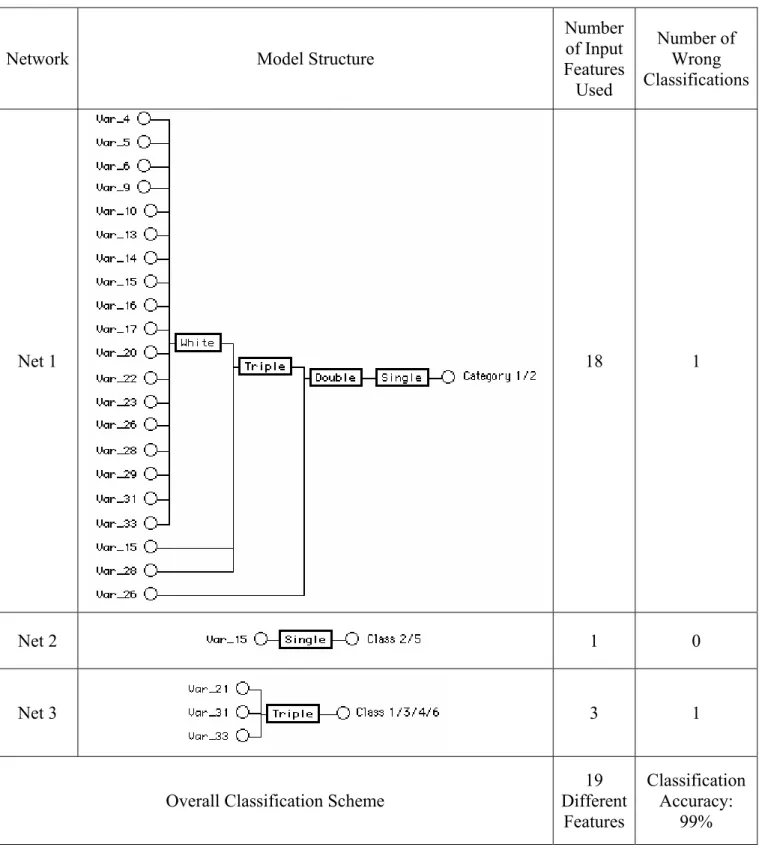
Table 6 shows model structures for the three classifier modules, all synthesized at the default CPM value of 1, as well as their performance on the evaluation set of 100 cases. The total number of different input features required by the three models is 19 features, which is 70% of the number of features used by the monolithic model in Fig. 4. The subset of 15 discarded features is {1,2,3,7,8,11,12,18,19,24,25,27,30,32,34}, which includes 5 of the 9 features discarded by the data reduction procedure in [21]. Net 1 distinguishes between the two main disorder categories with only one error, and is the most complex of the three models. Identifying classes within each group proves to be a much simpler task. Net 2 is a single element model that discriminates between classes 2 and 5 in the Eczema group with 100% accuracy using only feature 15 (Fibrosis of the papillary dermis). Fibrosis of dermal papillae is the predominant feature in chronic dermatitis as it represents the cutaneous reaction to chronic itching and rubbing of the skin. Inspection of the full data set revealed that the value of feature 15 is 0 for all class 2 cases and > 0 for all class 5 cases. Referring to the approximate profiling column in Table 5, it is noted that feature 15 forms the intersection of the two feature subsets characterizing classes 2 and 5. Net 3 is a single element, 3-input model that uses features 21, 31, and 33 to classify all four classes of the Papulosquamous group with only one error. Overall accuracy of the problem decomposition classification scheme is 99%, which matches the theoretical upper bound proposed by West and West [21]. The confusion matrix giving details of the classification performance is shown in Table 3(c). A 3-member committee of abductive networks trained on different subsets of the same dataset achieved classification accuracy of only 93% [26].

4.3.2. Separability-based Hierarchical Problem Decomposition

With this approach, the six disorders of the dermatology dataset are partitioned into two categories based on class separability properties reported by West & West [21]. Their exploratory data

analysis performed on the dataset using SOM maps revealed that four classes, namely 1 (Psoriasis), 3 (Lichen Planus), 5 (Chronic Dermatitis), and 6 (Pityriasis Rubra Pilaris) are quite distinct. They conclude that most of the error in conventional classification systems results from confusion in separating the two remaining classes, namely 2 (Seborrheic Dermatitis) and 4 (Pityriasis Rosea) which partially overlap. Effective improvement in the overall classification accuracy for the dataset should address the issue of poor separability between classes 2 and 4. They employed a back propagation neural network classifier augmented by a mixture-of-experts network for enhancing the separation of the two overlapping classes. Here we propose a two-stage hierarchical problem decomposition classification scheme based on their findings, with class subsets {2,4} and {1,3,5,6} forming category 1 and category 2, respectively. This allows handling classes 2 and 4 by a dedicated classifier optimized for their adequate separation at the second classifier stage.

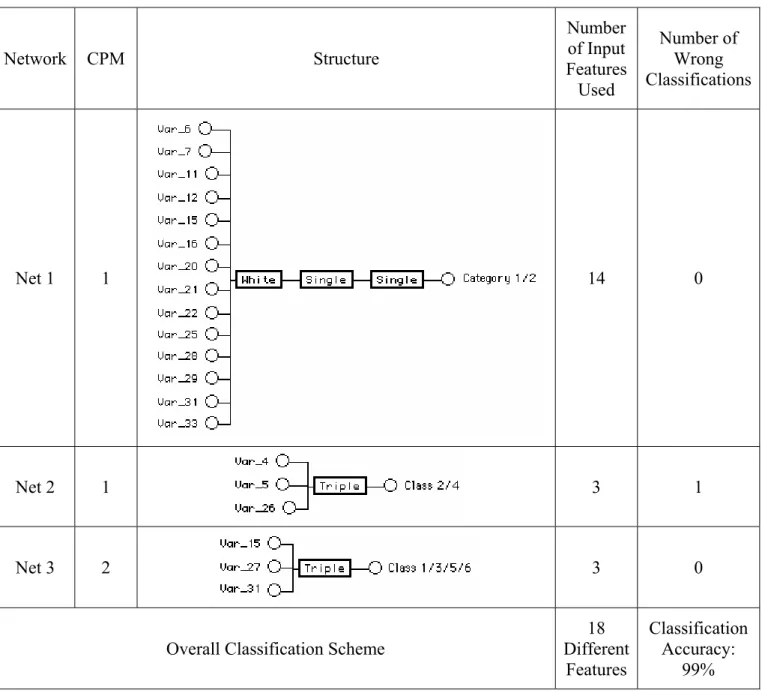
Table 7 shows model structures for the three classifier modules, the CPM value used, as well as their performance on the evaluation set of 100 cases. The total number of different input features required by the three models is 18 features, amounting to two thirds of features used by the monolithic model in Fig. 4. Out of the 18 features used by this classifier, 13 have been used by that described in Section 4.3.1. The subset of 16 discarded features is {1,2,3,8,9,10,13,14,17,18,19,23,24,30,32,34}, which includes 8 of the 9 features discarded by the data reduction procedure in [21]. Net 1 distinguishes between the two main disorder categories with 100% accuracy, and is the most complex of the three models. However, this 14-input, 3-layer model is simpler than the corresponding 18-input, 4-layer model for the other problem decomposition approach described in Section 4.3.1. Identifying classes within each group proves to be a much simpler task. Both Net 2 and Net 3 are single element, 3-input models. Net 2 classifies classes 2 and 4 with a single error while Net 3 classifies classes 1, 3, 5, and 6 with no errors. The optimum form of Net 3 was synthesized with CPM = 2 (i.e. is a simpler model than Net 2). These two observations confirm the fact that category 2 classes are easier to

separate than category 1 classes. Net 2 uses features 4, 5, and 26 to separate class 2 from class 4. Referring to the approximate profiling column in Table 5, it is noted that feature 5 forms part of the intersection between the two feature subsets characterizing classes 2 and 4. Inspection of the full data set revealed that the value of feature 5 has averages of 0.033 and 1.167 and standard deviations of 0.258 and 0.808 for classes 2 and 4, respectively. Using the number of cases given in Table 2 for the two classes in the total dataset, the z-statistic shows the difference between the means of the two features statistically significant at the 99% confidence level (α = 0.01). Overall accuracy of the problem decomposition classification scheme is 99%, which is identical to that achieved by the other problem decomposition approach of Section 4.3.1. The confusion matrix giving details of the classification performance is shown in Table 3(d).

5. Conclusions

Problem decomposition offers several advantages in dealing with the difficult problem of diagnosing multiple disorders of similar symptoms and signs. Starting by judiciously decomposing the problem into simpler subtasks, the whole exercise instills better understanding of the diagnosis problem. Simpler classifier models handling the smaller subtasks perform better and should execute faster. With GMDH-based abductive networks, automatic selection of only relevant inputs validates knowledge on the diagnostic value of disease markers, simplifies classification models, and helps explain and justify diagnostic decisions. In addition to improving classifier performance, the resulting data reduction helps simplify, and reduce the cost of, diagnostic tests required and offset the problems of high dimensionality, e.g. by allowing adequate training on smaller datasets. We have demonstrated the effectiveness of hierarchical classifiers employing problem decomposition approaches in improving the performance and reducing the cost of classifying multiple disorders of a standard dermatology dataset. Clinical-based and informatics-based problem decompositions achieved up to 47% reduction in the number of features used and 99% classification accuracy. The latter value is a

theoretical upper limit reported in the literature. This accuracy far exceeds that of monolithic models as well as network ensembles trained on different subsets of the dataset. Findings on the diagnostic value of various features agree with clinical knowledge and with results from previous studies on the dataset. It was found that the histopathological feature number 15 (Fibrosis of the papillary dermis) alone could discrminate between class 2 (Seborrheic Dermatitis) and class 5 (Chronic Dermatitis) with 100% accuracy. Simple classifier models can be represented as manageable analytical relationships that directly relate the classsifier output to the relevant input features. Future work would apply similar approaches to other mutliclass medical data such as the thyroid dataset.

Acknowledgement

The first author wishes to acknowledge the support of the Computer Engineering Department and the Research Committee at King Fahd University of Petroleum and Minerals, Dhahran, Saudi Arabia.

References

[1] Wu TD. A problem decomposition method for efficient diagnosis and interpretation of multiple disorders. Computer Methods and Programs in Biomedicine 1991;35:239-50.

[2] Ohno-Machado L, Musen MA. Hierarchical neural networks for partial diagnosis in medicine. World Congress on Neural Networks, 1994, 291-6.

[3] Gorry GA. Strategies for computer-aided diagnosis. Math. Biosci. 1968;2:293-318.

[4] Weiss SM, Kulinowski CA, Amarel S, Safir A. A model-based method for computer-aided medical decision making. Artificial Intelligence 1978;11:145-72.

[5] Montgomery GJ, Drake KC. Abductive networks. Proceedings of the SPIE Conference on the Applications of Artificial Neural Networks, 1990, 56-64.

[6] Farlow SJ. The GMDH algorithm. In: Farlow SJ, ed. Self-Organizing Methods in Modeling: GMDH Type Algorithms. New York: Marcel-Dekker, 1984:1-24.

[7] Abdel-Aal RE, Mangoud AM. Modeling obesity using abductive networks. Comput Biomed. Res. 1997;30:451-71.

[8] Abdel-Aal RE, Mangoud AM. Abductive machine learning for modeling and predicting the educational score in school health surveys. Methods Inf Med1996;35:265-71.

[9] Echauz J, Vachtsevanos G. Neural network detection of antiepileptic drugs from a single EEG trace. Proceedings of the Electro/94 International Conference, 1994, 346-51.

[10] Kondo T, Pandya AS, Zurada JM. GMDH-type neural networks and their application to the medical image recognition of the lungs. Proceedings of the 38th IEEE SICE Annual Conference,

1999, 1181-6.

[11] Cheung J, Lin ZY, McCallum RW, Chen JDZ. Screening of delayed gastric emptying using electrogastrography andabductivenetworks. Gastroenterology Suppl. S 1997;112:A711.

[12] Karlik B and Ozbay Y. A new approach for arrhythmia classification. 18th Annual International Conference of the IEEE Engineering in Medicine and Biology Society, 1996, 1646-7.

[13] Syiam MM. A neural network expert system for diagnosing eye diseases. Proceedings of the 10th Conference on Artificial Intelligence for Applications, 1994, 491-2.

[14] Nguyen HT, Butler M, Roychoudhry A, Shannon AG, Flack J, Mitchell P. Classification of diabetic retinopathy using neural networks. Proceedings of the 18th Annual International Conference of the IEEE Engineering in Medicine and Biology Society: Bridging Disciplines for Biomedicine, 1996, 1548-9.

[15] Ramadan Z, Ropella K, Myklebust J, Goldstein M, Feng X, Flynn J. A neural network to discriminate between dyslexic subtypes, Annual International Conference of the IEEE Engineering in medicine and Biology Society, 1991, pp. 1405-6.

[16] Axer H, Jantzen J, Berks G, v. Keyserlingk DG. Aphasia Classification Using Neural Networks. Proc. of ESIT 2000, Aachen, Germany, 2000, 111-5.

[17] Kim BY, Park KS. Automatic sleep stage scoring system using genetic algorithms and neural network. Proceedings of the 22nd Annual International Conference of the IEEE Engineering in Medicine and Biology Society, 2000, 849-50.

[18] Abe H, Ashizawa K, Li F, Matsuyama N, Fukushima A, Shiraishi J, MacMahon H, Doi K. Artificial neural networks (ANNs) for differential diagnosis of interstitial lung disease: results of a simulation test with actual clinical cases. Academic Radiology 2004;11:29-37.

[19] García-Pérez E, Violante A, Cervantes-Pérez F. Using neural networks for differential diagnosis of Alzheimer disease and vascular dementia. Expert Systems with Applications 1998;14:219-25.

[20] Ikeda M , Ito S, Ishigaki T, Yamauchi K. Evaluation of a neural network classifier for pancreatic masses based on CT findings. Computerized Medical Imaging and Graphics 1997;21:175-83.

[21] West D, West V. Improving diagnostic accuracy using a hierarchical neural network to model decision subtasks. International Journal of Medical Informatics 2000;57:41-55.

[22] Pratt LY, Kamm CA. Improving a phoneme classification neural network through problem decomposition, IJCNN-91-Seattle International Joint Conference on Neural Networks, 1991, 821-826. [23] Wen H, Ozdamar O. Auditory brainstem response classification using modular neural networks.

Proceedings of the Annual International Conference of the IEEE Engineering in Medicine and Biology Society, 1991, 1879-80.

[24] Chi Z, Jabri MA. Identification of supraventricular and ventricular arrhythmias using a combination of three neural networks. Proceedings of the IEEE Conference on Computers in

Cardiology, 1991, 169-72.

[25] Guan S –U, Li S. Parallel growing and training of neural networks using output parallelism, IEEE Transactions on Neural Networks 2002;13:542–50.

[26] Abdel-Aal RE. Abductive network committees for improved classification of medical data. Methods of Information in Medicine 2004;43:192-201.

[27] Lee C-C, Chung P-C, Tsai H-M. Identifying multiple abdominal organs from CT image series using a multimodule contextual neural network and spatial fuzzy rules. IEEE Transactions on Information Technology in Biomedicine 2003;7:208–17.

[28] Guvenir HA, Demiroz G and Ilter N. Learning differential diagnosis of erythemato-squamous diseases using voting feature intervals. Artificial Intelligence in Medicine 1998;13:147-65.

[29] Abdel-Aal RE. Experimental evaluation of performance improvements in abductive network classifiers with problem decomposition. Neurocomputing 2004;61: 193-215.

[30] AbTech Corporation, Charlottesville, VA, AIM User's Manual, 1990.

[31] Barron AR. Predicted squared error- a criterion for automatic model selection. In: Farlow SJ, ed. Self-Organizing Methods in Modeling: GMDH Type Algorithms. New York: Marcel-Dekker, 1984:87-103.

[32] Anand R., Mehrotra K, Mohan CK, Ranka S. Efficient classification for multiclass problems using modular neural networks. IEEE Transactions on Neural Networks 1995;6:117-24.

[33] http://www.ics.uci.edu/~mlearn/MLRepository.html.

[34] Bojarczuk CC, Lopes HS, Freitas AA, Michalkiewicz EL. A constrained-syntax genetic programming system for discovering classification rules: application to medical data sets. Artificial

Intelligence in Medicine 2004;30:27-48.

[35] Karayiannis NB, Randolph-Gips MM. On the construction and training of reformulated radial basis function neural networks. IEEE Transactions on Neural Networks 2003;14:835-46. [36] Braun-Falco O, Christophers E. Arch Dermatol Forsch. 1974;251:95-110.

[37] Ragaz A, Ackerman AG. Evolution, maturation and regression of lesions of psoriasis. Aust J Dermopathol 1979;1:198-203.

[38] Valdes-Perez RE, Pericliev V, Pereira F. Concise. Intelligible, and approximate profiling of multiple classes. International Journal of Human Computer Systems 2000;53:411-36.

[39] Fidelis MV, Lopes HS, Freitas AA. Discovering comprehensible classification rules with a genetic algorithm.Proceedings of the IEEE Congress on Evolutionary Computation, 2000, 805-10. [40] Lever WF. Lever's Histopathology of the Skin, 8th Edition, J.B. Lippincott, 1996.

Table 1. Brief description of the dataset input features. All features take the value 0, 1, 2, or 3, except family history (0 or 1) and age which takes integer values in the range 0 to 70 years.

Feature Number in Dataset Name 1 Erythema 2 Scaling 3 Definite borders 4 Itching 5 Koebner phenomenon 6 Polygonal papules 7 Follicular papules 8 Oral mucosal involvement 9 Knee and elbow involvement 10 Scalp involvement 11 Family history

12 Melanin incontinence 13 Eosinophils in the infiltrate 14 PNL infiltrate

15 Fibrosis of the papillary dermis 16 Exocytosis

17 Acanthosis 18 Hyperkeratosis 19 Parakeratosis 20 Clubbing of the rete ridges 21 Elongation of the rete ridges

22 Thinning of the suprapapillary epidermis 23 Spongiform pustule

24 Munro microabcess 25 Focal hypergranulosis 26 Disappearance of the granular layer 27 Vacuolisation and damage of basal layer 28 Spongiosis

29 Saw-tooth appearance of retes 30 Follicular horn plug

31 Perifollicular parakeratosis

32 Inflammatory monoluclear inflitrate 33 Band-like infiltrate

Table 2. Distribution of the six output classes in the total, training, and evaluation datasets. Total Dataset (358 Cases) Training Set (258 Cases) Evaluation Set (100 Cases) Code Class Number

of Cases Prevalence, % Number of Cases Prevalence, % Number of Cases Prevalence, % 1 Psoriasis 111 31.0 77 29.9 34 34.0

2 Seborrheic _Dermatitis 60 16.8 45 17.5 15 15.0 3 Lichen _Planus 71 19.8 55 21.3 16 16.0 4 Pityriasis _Rosea 48 13.4 38 14.7 10 10.0 5 _Dermatitis Chronic 48 13.4 30 11.6 18 18.0 6 _{Rubra Pilaris} Pityriasis 20 5.6 13 5.0 7 7.0

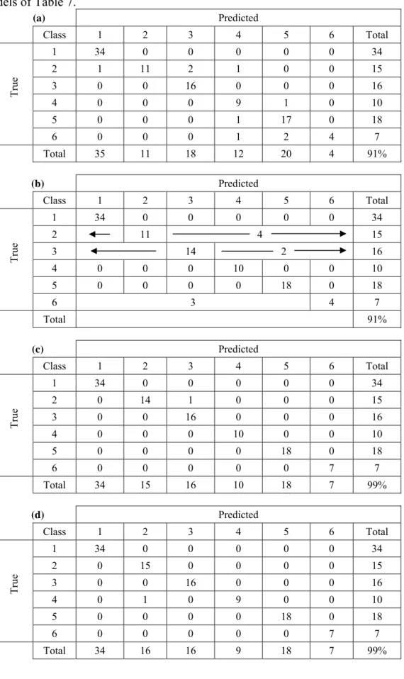
Table 3. Confusion matrices showing detailed classification performance for: (a) Monolithic model of Fig. 4, (b) Class decomposition models of Table 4, (c) Clinical-based hierarchical problem decomposition models of Table 6, and (d) Separability-based hierarchical problem decomposition models of Table 7. (a) Predicted Class 1 2 3 4 5 6 Total 1 34 0 0 0 0 0 34 2 1 11 2 1 0 0 15 3 0 0 16 0 0 0 16 4 0 0 0 9 1 0 10 5 0 0 0 1 17 0 18 Tr ue 6 0 0 0 1 2 4 7 Total 35 11 18 12 20 4 91% (b) Predicted Class 1 2 3 4 5 6 Total 1 34 0 0 0 0 0 34 2 11 4 15 3 14 2 16 4 0 0 0 10 0 0 10 5 0 0 0 0 18 0 18 Tr ue 6 3 4 7 Total 91% (c) Predicted Class 1 2 3 4 5 6 Total 1 34 0 0 0 0 0 34 2 0 14 1 0 0 0 15 3 0 0 16 0 0 0 16 4 0 0 0 10 0 0 10 5 0 0 0 0 18 0 18 Tr ue 6 0 0 0 0 0 7 7 Total 34 15 16 10 18 7 99% (d) Predicted Class 1 2 3 4 5 6 Total 1 34 0 0 0 0 0 34 2 0 15 0 0 0 0 15 3 0 0 16 0 0 0 16 4 0 1 0 9 0 0 10 5 0 0 0 0 18 0 18 Tr ue 6 0 0 0 0 0 7 7 Total 34 16 16 9 18 7 99%

Table 4. Structures and performance of the modular classifiers synthesized with the class decomposition approach.

Class Model Structure

Number of Input Features Used Number of Wrong Classifications (/100 cases of the evaluation set) Class 1 4 0 Class 2 20 4 Class 3 1 2 Class 4 23 0 Class 5 2 0 Class 6 1 3

Overall Classification Scheme Different 28 Features

Classification Accuracy: 91%

Table. 5. Comparison of the features selected to represent each of the dermatology classes by the class decomposition approach, the approximate profiling approach [38], and the classification rule approach [39].

Classification Rules [39] Class Class Decomposition _{Profiling [38]} Approximate

Features Used _{Testing Set} Fitness on 1 (Psoriasis) {20,22,28,31} {22} {20,31} 0.973 2 (Seborrheic Dermatitis) {1,3,4,5,6,8,9,12,13, 14,15,16,18,19,20,23,26,28,31,33} {5,15,22,33,34} {5,27,28} 0.855 3 (Lichen Planus) {33} {33} {33} 0.979 4 (Pityriasis Rosea) {1,2,4,5,7,8,9,13,14, 15,17,19,20,21,22,23,25,26,27,28, 29,31,33} {5,22,33} {9,11,17,25,28,_32} 0.783 5 (Chronic Dermatitis) {5,15} {15} {12,15,24} 1.000 6 (Pityriasis Rubra Pilaris) {31} {34} {7,31} 1.000

Table 6. Structures and performance of the modular classifiers synthesized for the clinical-based hierarchical problem decomposition.

Network Model Structure

Number of Input Features Used Number of Wrong Classifications Net 1 18 1 Net 2 1 0 Net 3 3 1

Overall Classification Scheme

19 Different Features Classification Accuracy: 99%

Table 7. Structures and performance of the modular classifiers synthesized for the separability-based problem decomposition.

Network CPM Structure Number of Input Features Used Number of Wrong Classifications Net 1 1 14 0 Net 2 1 3 1 Net 3 2 3 0

Overall Classification Scheme

18 Different Features Classification Accuracy: 99%

Input Vector Class 1 Classifier Net 1 Class 2 Classifier Class 2 Net 2 Class i Classifier Class i Net i Class K Class K Classifier Net K Class 1

Input Vector Level 1 Classifier: Category 1/ Category 2 Category 2 Classes Level 2 Classifier for Category 1 Net 3 Level 2 Classifier for Category 2 Category 1 Enable Category 2 Enable 2 Net 1 Net Category 1 Classes

Fig. 3. A schematic diagram showing a two-stage hierarchical problem decomposition approach to multiclass classification