Washington University in St. Louis
Washington University Open Scholarship
Engineering and Applied Science Theses &
Dissertations McKelvey School of Engineering
Winter 12-15-2014
Approximation and Relaxation Approaches for
Parallel and Distributed Machine Learning
Stephen Tyree
Washington University in St. Louis
Follow this and additional works at:https://openscholarship.wustl.edu/eng_etds
Part of theEngineering Commons
This Dissertation is brought to you for free and open access by the McKelvey School of Engineering at Washington University Open Scholarship. It has Recommended Citation
Tyree, Stephen, "Approximation and Relaxation Approaches for Parallel and Distributed Machine Learning" (2014).Engineering and Applied Science Theses & Dissertations. 64.
WASHINGTON UNIVERSITY IN ST. LOUIS
School of Engineering and Applied Science Department of Computer Science and Engineering
Dissertation Examination Committee: Kilian Q. Weinberger, Chair
Kunal Agrawal Roger Chamberlain Laurens van der Maaten
Robert Pless
Approximation and Relaxation Approaches for Parallel and Distributed Machine Learning by
Stephen W. Tyree
A dissertation presented to the Graduate School of Arts and Sciences
of Washington University in partial fulfillment of the requirements for the degree
of Doctor of Philosophy
December 2014 St. Louis, Missouri
c
Contents
List of Figures . . . iv List of Tables . . . v Acknowledgments . . . vi Abstract . . . x 1 Introduction . . . 11.1 Learning from Data . . . 3
1.2 Non-Linear Machine Learning Methods . . . 7
1.3 Parallel and Distributed Systems . . . 14
2 Parallel Boosted Tree Ensemble Construction . . . 17
2.1 Gradient Boosted Regression Trees . . . 19
2.1.1 Notation . . . 19
2.1.2 Gradient Boosting . . . 21
2.1.3 Regression Trees . . . 24
2.2 Related Work . . . 31
2.3 Feature-wise Distribution . . . 34
2.4 Instance-wise Distribution with Histograms . . . 37
2.4.1 Setting . . . 39
2.4.2 Cumulative Statistics . . . 41
2.4.3 Histograms . . . 43
2.5 Experimental Results . . . 50
2.5.1 Web Search Ranking . . . 51
2.5.2 Data Sets . . . 55
2.5.3 Experimental Setup . . . 55
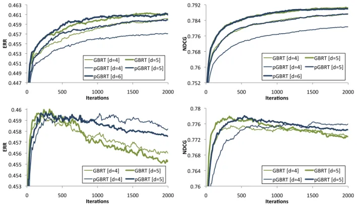
2.5.4 Prediction Accuracy . . . 57
2.5.5 Performance and Speedup . . . 60
2.6 Discussion . . . 64
3 Parallel Non-Linear Metric Learning with Boosted Tree Ensembles . . . 66
3.1 Introduction . . . 67
3.2.1 Background . . . 72
3.2.2 Related Work . . . 74
3.2.3 Non-linear Transformations with Gradient Boosting . . . 75
3.2.4 Experimental Results . . . 80
3.2.5 Discussion . . . 84
3.3 Random Forest Ensemble Metrics . . . 84
3.3.1 Background and Related Work . . . 88
3.3.2 Methods . . . 93
3.3.3 Experimental Results . . . 101
3.3.4 Discussion . . . 109
4 Multi-Platform Parallelism for Support Vector Machines . . . 112
4.1 Introduction . . . 113
4.2 Parallelism for GPUs and Multicores . . . 120
4.2.1 Explicitly Parallel SVM Optimization . . . 120
4.2.2 Implicitly Parallel SVM Optimization . . . 122
4.2.3 Implementing Sparse-Primal SVM . . . 125
4.3 Experimental Results . . . 131
4.4 Discussion . . . 138
5 Conclusions . . . 140
List of Figures
1.1 The “XOR” dataset and three non-linear models. . . 8
2.1 A simple regression tree. . . 25
2.2 ERR and NDCG for Yahoo Sets 1 and 2 on parallel and exact implementations for varying tree depths. . . 57
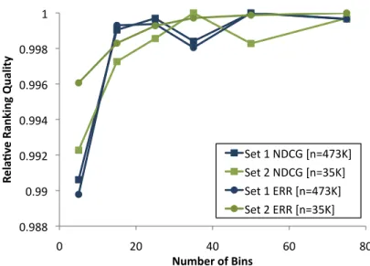
2.3 Ranking performance of pGBRT on the Yahoo Sets 1 and 2 with a varying number of histogram bins. . . 61
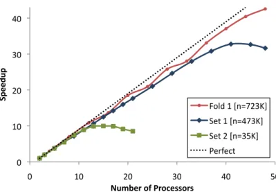
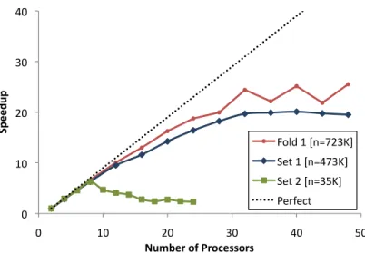
2.4 The speedup of pGBRT on a multicore shared memory machine. . . 62
2.5 The speedup of pGBRT on a distributed memory cluster. . . 63
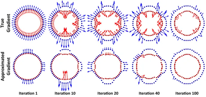
3.1 GB-LMNN illustrated on a toy data set. . . 78
3.2 Sensitivity of GB-LMNN to the tree depth parameter. . . 83
3.3 Random forest schematic showing posterior label predictions made at each tree. 88 3.4 Test error of RFEM with a varying number of trees. . . 106
3.5 RFEM and Euclidean metrics applied to Yale Faces test instances. . . 107
3.6 t-SNE visualization of four test data sets using Euclidean distance, LMNN distance, and RFEM distance. . . 111
List of Tables
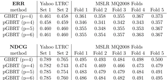
2.1 Statistics of the Yahoo and Microsoft Learning to Rank data sets. . . 55 2.2 Results in ERR and NDCG on the Yahoo and Microsoft data sets. . . 58 3.1 kNN classification error for linear and nonlinear metric learning methods. . . 81 3.2 kNN classification error with dimensionality reduction to output
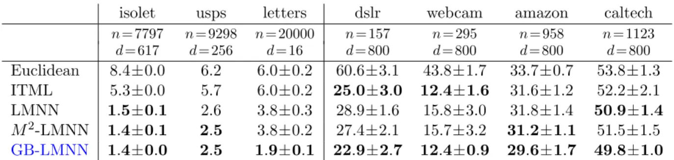
dimension-ality r. . . 82 3.3 Dataset attributes and test error rates of kNN classifiers using seven metric
learning approaches. . . 103 3.4 Test error with RFEM using five different histogram distances. . . 105 3.5 Test error on classes held out during training. . . 108
4.1 Comparison of test error, training time, and speedup of kernelized SVM train-ing methods. . . 132
Acknowledgments
At first glance, this dissertation may seem to be the result of copious coffee, computer code,
and server time. (That there was much coffee is certain.) But more than that, this particular
dissertation the result of relationships. To begin, I owe much to the professor who taught a
remarkably exciting class in machine learning my first semester (Kilian), therein completely
changing my desired research direction. My debt is extended to the colleague (Kunal) he
asked to sign on to collaboratively co-advise me. Their commitment to my development and
success through thick and thin have brought me to this point.
My lab-mates in Kilian’s group have been the best colleagues and friends I could have hoped
for in a graduate program. Mimmin, Eddie (Zhixiang), Dor, Matt, Jake, and Wenlin: our
collaborations have truly been the highlight of my time here. Austin, David, Mithun,
Shau-rya, Steve, Zheng, and various others (graduate students, undergraduates, and visitors) that
I have befriended along the way: best of luck and godspeed. I must also acknowledge my
dissertation committee: thank you for granting me your time and support. I am very
grate-ful to NVIDIA both for the funding and opportunities afforded by the NVIDIA Graduate
This long journey to a dissertation began at home, with encouragement and support from my
parents, much love from grandparents, and affectionate goads from my two younger brothers.
I am proud of each of you and am grateful to have made you proud of me in turn.
From almost the very start, I have been incredibly blessed to have two extended families in
St. Louis. International Friends has taught me the bittersweet reality of a world that is at
once so very small and so very big. Aigula, Alicia, Allison, Andrea, Arpith, Brian, Carol,
Chenyu, Chioma, Chui Li, Dale, Esha, Fernando, Foster, Hyunju, Ifeoma, Josh, Nicolas,
Ophelia, Pato, Rachel, Rodger, Seth, Sharleen, Silvana, Stan, and Vernal: thank you for
showing and leading me in grace, peace, and love. I can personally attest, “Where morning
dawns, where evening fades, You call forth songs of joy.” (Psalm 65:8)
My second St. Louis family is New City Fellowship, specifically the Koch-Woodard house
church. David, Mandy, Timothy, Christopher, and Karis; Mark, Aubree, Wendy, and Lucy;
Matt and Nicole; Sally; Paul and Kathy; and Erin: you are each dear to my heart and
bring countless smiles to my face, “For you yourselves have been taught by God to love each
other.” (1 Thessalonians 4:9) As we walk together, always remember, “He will bring forth
I cannot possibly name everyone whose support and companionship I have received while
trudging this “road of happy destiny,” but I am immensely grateful to have encountered each
of you. This work is a testament to your friendship and support.
Stephen W. Tyree
Washington University in St. Louis December 2014
“For us, there is only the trying. The rest is not our business.”
ABSTRACT OF THE DISSERTATION
Approximation and Relaxation Approaches for Parallel and Distributed Machine Learning by
Stephen W. Tyree
Doctor of Philosophy in Computer Science Washington University in St. Louis, 2014
Professor Kilian Q. Weinberger, Chair
Large scale machine learning requires tradeoffs. Commonly this tradeoff has led practition-ers to choose simpler, less powerful models, e.g. linear models, in order to process more training examples in a limited time. In this work, we introduce parallelism to the training of non-linear models by leveraging a different tradeoff—approximation. We demonstrate var-ious techniques by which non-linear models can be made amenable to larger data sets and significantly more training parallelism by strategically introducing approximation in certain optimization steps.
For gradient boosted regression tree ensembles, we replace precise selection of tree splits with a coarse-grained, approximate split selection, yielding both faster sequential training and a significant increase in parallelism, in the distributed setting in particular. For metric learning with nearest neighbor classification, rather than explicitly train a neighborhood structure we leverage the implicit neighborhood structure induced by task-specific random forest classifiers, yielding a highly parallel method for metric learning. For support vector machines, we follow existing work to learn a reduced basis set with extremely high parallelism, particularly on GPUs, via existing linear algebra libraries.
We believe these optimization tradeoffs are widely applicable wherever machine learning is put in practice in large scale settings. By carefully introducing approximation, we also intro-duce significantly higher parallelism and consequently can process more training examples for more iterations than competing exact methods. While seemingly learning the model with less precision, this tradeoff often yields noticeably higher accuracy under a restricted training time budget.
Chapter 1
Introduction
Large scale machine learning requires tradeoffs. Commonly this tradeoff has led
practition-ers to choose simpler, less powerful models, e.g. linear models, in order to process more
training examples in a limited time. In this work, we introduce parallelism to the training
of non-linear models by resorting to a different tradeoff—approximation. We demonstrate
various techniques by which non-linear models can be made amenable to larger data sets and
added parallelism by strategically introducing approximation in certain optimization steps.
In practice, the combination of increased non-linear model power and the ability to train
on more data counteract the loss of precision due to approximation. The result is higher
accuracy in training time which is competitive with less powerful methods.
For gradient boosted regression tree ensembles, we consider trading off the precise selection
of tree splits in favor of a coarse-grained, approximate split selection. This opens the door
setting in particular. While the consequence is a small loss in accuracy, boosted tree
ensem-bles are shown to be highly resilient to this approximation and significantly more parallel as
a result. We leverage this method for both large scale regression (e.g. learning to rank) and
non-linear metric learning.
For metric learning with nearest neighbor classification, it is common to learn a metric
which explicitly produces some desired neighborhood structure. However, this is often both
computationally expensive and limited in parallelism. In this work, we opt out entirely from
the optimization of an explicit neighborhood structure. Instead, we leverage the implicit
neighborhood structure induced by task-specific random forest classifiers. In doing so, we
co-opt the highly parallel random forest training procedure to metric learning. The result is an
accurate metric for nearest neighbor classification and an additional layer of interpretability
for random forest predictions.
For support vector machines, previous work has shown that adopting a carefully selected
reduced basis set, instead of learning weights for all support vectors, can maintain high
accuracy while significantly reducing training time and model size. We leverage this existing
work and demonstrate that this training also presents extremely high parallelism, particularly
on GPUs. Further, the method suffers little loss in accuracy under additional approximation
by choosing the basis vector set with only minor supervision or even randomly. The result is
the fastest publicly-available kernel SVM training code released to date for either multicore
We believe these optimization tradeoffs are widely applicable wherever machine learning
is put in practice in large scale settings. By carefully introducing approximation, we also
introduce significantly higher parallelism and consequently can process more data examples
for more iterations than competing exact methods. While seemingly learning the model
with less precision, this tradeoff often yieldshigher accuracy under a restricted training time
budget.
In the remainder of this chapter, we introduce the general problem of learning predictors
from data, along with several common methods for learning non-linear predictors. Finally, we
consider a variety of settings for parallel and distributed computing which will be leveraged
throughout this dissertation.
1.1
Learning from Data
With many complex tasks, it is remarkably challenging to precisely describe how to
accom-plish the task, e.g. in a computer program. For example, it would be very difficult to write
a computer program which takes as input the image of a handwritten digit and returns the
value of the digit represented in the image. (Indeed, it is hard to convey the same task to
young humans.)
Yet, for many complex problems, it is almost trivial to accumulate examples of the
straightforward to collect numerous examples of handwritten digits with the identity of the
digit written in each. Indeed, far more humans are capable of creating or collecting such
examples than have sufficient skills to write complex computer code.
With this setup, we no longer want to write a digit recognition program by hand. Rather, if
we could leverage a more general, existing program—a pattern recognition method—we could
present our collection of task examples and allow the general program to learn the pattern
behind the examples in order to repeat the task on new examples. Then, the handwritten
digit task becomes a data collection and labeling problem rather than a challenging reasoning
and programming task!
Supervised learning. Supervised machine learning is concerned with designing pattern
recognition methods. We assume we are presented with examples of the inputs to and
outputs from a function of unknown form. Examples of functions of interest may include:
• the identity of a handwritten digit in an image;
• whether an email message is or is not spam; and
• the relevance of a document to a web search query string.
In each case, these functions are hard to characterize directly, yet it may be quite simple to
• recruiting several hundred subjects and asking each to write the digits 0-9;
• recording which emails are marked spam by users of a web-based email service; and
• examining click-through rates and human evaluator scores on web search results.
Data and learning problems. In the machine learning context, a set of input and output
pairs constitutes atraining set. A machine learning algorithm attempts to approximate the
unknown function underlying the training data, capturing a model for the function. When
presented with a previously unseen input, referred to as a test input, the model is used to
predict the function’s output.
We assume training data D = {(xi, yi)} n
i=1 are in the form of n samples from some input
distribution. The samples are captured as feature vectors xi ∈ X ⊆ Rd in a d-dimensional
vector space. We denote the value of featurej of sampleiby the notation [xi]j. Each sample
xi is associated with a label yi ∈ Y, an observed output of the function to be learned when
queried with input xi. This label yi indicates the property we would like to automatically
predict about unlabeled instances.
When the set of label values is an ordered subset of the real numbers (Y ⊆R), we refer to
the problem as a regression problem. When the set of label values is discrete and unordered
(Y ∈ {1,2, ..., c}), we refer to the discrete labels asclasses and the problem as aclassification
multiclass problems can be (and often are) solved as a series of binary classification problems
[69, 151].
Learning as optimization. The goal is to learn a functionh:X → Y such that h(xi)≈
yi. We choose our predictorhfrom some restricted class of functionsH. A common approach
is to optimize the predictor h with respect to a cost function C(h), selecting the function ˆh
which minimizes the mis-prediction cost on the available training instances:
ˆ
h= argmin
h∈H
C(h).
For many cost functions, this optimization is intractable. This includes, for example, the
most straightforward classification error measure, the mis-prediction count:
C(h) =
n
X
i=1
[h(xi)6=yi],
where [·] denotes the Iverson bracket. Mis-prediction counts are non-continuous in the space
of predictor functions, as a small change in predictor output may induce large changes in
the cost function. Without a well-behaved error measure, function selection can become a
One solution is to optimizeh with respect to a well-behaved surrogate cost function C(h)— continuous, at least once differentiable, and (ideally) convex. Surrogate cost functions
com-monly upper bound the desired error measure. With such a function, learning predictors in
many function classes is a numerical minimization problem amenable to well-studied first- or
second-order mathematical optimization methods, including gradient descent and Newton’s
method. One typical well-behaved cost function for regression problems is the squared-loss,
C(h) =
n
X
i=1
(h(xi)−yi)2.
Several cost functions are common for learning classification models, including the logistic,
exponential, and hinge loss functions.
1.2
Non-Linear Machine Learning Methods
Machine learning is extremely effective for a wide variety of data analysis and prediction
tasks. For many complex problems, non-linear models have proven essential to achieving
high prediction accuracy. In this context, non-linearity refers to the ability to capture effects
which cannot be modeled as a linear combination of features in the input spaceX. Consider
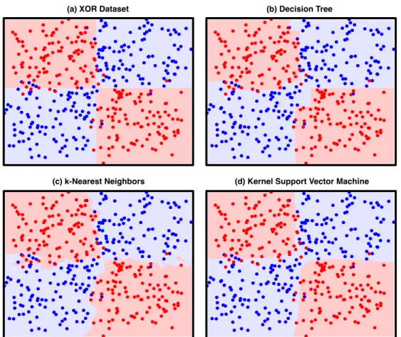
a version of the “XOR-problem” as depicted in Figure 1.1(a). No linear combination of the
(a) XOR Dataset (b) Decision Tree
(c) k-Nearest Neighbors (d) Kernel Support Vector Machine
Figure 1.1: A simple noisy “XOR” dataset with two classes (red and blue dots), and the decision boundary (red and blue shading) of (a) the underlying noiseless “XOR” distribution, (b) a decision tree, (c) the k-nearest neighbors decision rule (k = 3), and a kernel support vector machine (C = 1, γ = 1).
depicted in Figure 1.1(b-d) and discussed in the following paragraphs, models learned from
a variety of non-linear function spaces can easily produce reliable predictors.
Learning non-linear models often presents significant computational challenges, particularly
when paired with large-scale training sets. The work in this dissertation encompasses several
to effectively speed up and scale up machine learning with non-linear models. Here we discuss
three categories of non-linear models which will be referenced in subsequent chapters.
Decision trees and tree ensembles. Decision tree models operate by recursively
parti-tioning the feature space using axis-aligned splits. This input space partiparti-tioning is captured
in a binary tree structure. The tree’s internal nodes denote single-feature partitioning rules
of the form [x]j ≤ θ, where j is an index in feature vector x and θ is a split threshold.
Leaf nodes in the tree indicate prediction labels, with one constant label value
correspond-ing to each input space partition. Trees are denoted classification orregression trees based
on whether leaf predictions are class labels (or distributions over classes) or real numbers,
respectively.
A prediction is made for a samplexby descending the tree. Following the branching rule at
each internal node, the left child node is chosen when the rule evaluates true, otherwise the
right child is chosen. Upon reaching a leaf node, the leaf’s label is returned as the prediction.
Trees naturally capture non-linear decision boundaries, are invariant to feature scaling, and
readily incorporate a variety of input spaces including categorical features. Tree training is
typically accomplished via a top-down procedure which greedily chooses splits to minimize
prediction error at the next level of the tree. Construction of each level of nodes typically
involves a sequential pass over the training samples, considering the effect of each potential
easily capture smooth decision boundaries and, due in part to the greedy training procedure,
can easily “overfit” to specific patterns in the training set.
Tree ensemble models use a collection of subtly varying trees to learn powerful and easily
configured classifiers for many problems. Merging many trees supports smooth decision
boundaries. Fitting the trees to varying views of the training dataset helps to alleviate
overfitting. When trained bygradient boosting, trees in the ensemble are learned sequentially
to correct errors made by previous trees. Inrandom forests, a collection of “random” trees are
learned from different random samples from the training set and their predictions averaged.
When attempting to scale to large training sets, the sequential training of gradient boosting
places the burden of parallelization on the construction of individual trees. Leveraging special
properties of boosted tree models, particularly short tree depth and weak assumptions on
the accuracy of any individual tree, we present an extremely flexible approximate method to
parallelize tree learning in both distributed and multi-core settings. Random forest training
is naturally parallel as individual trees are learned on different independent samples from
the training set. We leverage parallelism in these methods to perform regression and metric
learning (as discussed in the next paragraph) on medium and large scale problems.
Nearest neighbor methods and metric learning. Nearest neighbor methods produce
arguably the simplest and most interpretable non-linear classification models. Predictions
to the unlabeled test instance, and constructing a prediction from the labels of the similar
examples.
For the case of 1-nearest neighbor classification (1NN), the predicted labelyt for a test point
xt is the label yi of the nearest training instancexi ∈ D:
yt= argmin (xi,yi)∈D
D(xt,xi),
for some distance functionD:X ×X → R+, effectively capturing inverse similarity. Common
choices for D(·) are the Euclidean distance for general vector data and the χ2 distance for
histograms or probability-vectors. In the general case of k-nearest neighbor classification (kNN), for somek≥1, classification predictions are made by a vote among the labels of the
k neighbors, while regression predictions are commonly produced by some form of averaging. The accuracy of nearest neighbor models relies heavily on the choice of similarity metric
for determining which neighbors are indeed “nearest” for both the sample input space and
the prediction task at hand. Metric learning optimizes task-specific similarity metrics to
minimize kNN error under the metric. It is often to useful to reframe the metric learning problem as learning a transformationφ(·) of the input feature space under which a standard metric, such as Euclidean or χ2, yields good kNN performance:
yt= argmin (xi,yi)∈D
Dφ(xt,xi) = argmin (xi,yi)∈D
In its simplest form, φ(·) is a linear transformation parameterized by matrix L: φ(x) =
Lx. Learning linear transformations presents computational advantages, however for some
problems the feature space cannot be adequately reshaped by simple linear manipulations.
In these cases, linear metric learning approaches, often corresponding to learning
non-linear transformations, can yield significant increases in accuracy. In this dissertation, we
introduce two novel non-linear metric learning approaches, each leveraging a parallel tree
ensemble approach for scalable training. Each approach yields highly competitive accuracy
with no significant parameters to tune and scalability to medium and large scale training
sets.
Kernel support vector machines. Support vector machines (SVM) learn a classifier
with a large “margin” between a linear hyperplane separating the two classes of samples and
the nearest training samples from each class. In the linear formulation, the SVM optimization
minimizes the hinge loss with respect to a linear hyperplane parameterized by weights w,
min w,b 1 2||w|| 2 2+C n X i=1 max(0,1−yi(w>xi+b)).
A maximum margin is enforced by L2-regularization on the hyperplane with tradeoff C. The “kernel trick” provides a natural non-linear extension to SVMs, implicitly learning a
hyperplane in a high (or even infinite) dimensional projection of the input space. In the
to the non-linear transformations discussed for metric learning. It is costly (or impossible
in the case of projections into infinite-dimensional feature spaces) to explicitly represent the
feature transformation and then proceed with SVM training. However, some transformations
have corresponding kernel functions, permitting closed-form solutions for inner products in
the transformed space, k(xi,xj) = φ(xi)>φ(xj). By solving the SVM optimization in the
dual [150] or by leveraging the Representer Theorem for primal optimization [47], training
samples are accessed only in inner product computations with other training samples,
per-mitting powerful non-linear projections by simply substituting a kernel function. As a result
of the kernel substitution, the hyperplane is represented as coefficients on kernel function
evaluations between training samples and a test sample. Training samples corresponding to
non-zero coefficients are called “support vectors.”
Quadratic model complexity and limited parallelism in typical SVM optimization procedures
have prevented the application of SVMs to many medium and large datasets. We review
the literature of SVM solvers seeking an SVM formulation and optimization method more
conducive to parallelism on modern multi-core and GPU hardware. By adopting a previously
published sparse SVM approximation, we successfully implement SVM training for
1.3
Parallel and Distributed Systems
Training speed is vital for practical machine learning settings. In many real-world
appli-cations, models are not simply trained once and reused ad infinitum. Rather, models are
frequently retrained as new labeled data are acquired. In adversarial settings or systems
whose behavior drifts over time, such as spam filtering or web search ranking, retraining
may occur at a daily or even hourly frequency to account for the changing environment.
Further, development and evaluation of new input features is a common process which also
requires model retraining.
Initial model training can exhibit some trivial parallelism when there are hyper-parameters to
tune. However, after hyper-parameter selection, a single training phase is typically engaged
using the full training set. Additionally, recent developments in Bayesian hyper-parameter
tuning [178] limit the need for broad searches over grids or random selections of
hyper-parameters. These observations solidify the need for fast, highly parallel training.
In conjunction, trends in computer architecture have been moving toward increasingly
par-allel hardware. Indeed the major speedups in hardware have been almost exclusively from
introducing more parallel cores rather than increasing the processing speed of individual
cores. In this dissertation, we explore parallelizations of a variety of non-linear learning
Thread and process level parallelism is supported in multiprocessing architectures, where
multiple processing cores are engaged simultaneously. Inshared memory architectures, these
cores are tightly coupled, having access to the same memory bus, and perhaps residing in the
same socket and sharing some level of the cache hierarchy. Communication among processors
is extremely fast, but system memory is limited by the amount of RAM configurable in a
single machine.
An extreme example of shared memory multiprocessing is found in general-purpose
graph-ics processing units (GPUs). GPUs were originally developed for real time rendering of
complex visual scenes from underlying 3-D shape models. As such, they have many hun-dreds of lightweight compute cores. Unlike traditional shared memory multi-core systems,
GPUs are optimized for high throughput. GPUs are based on a “same instruction
multi-ple data” (SIMD) architecture, which requires all threads within one block to execute the
exact same instructions, whereas multi-core CPUs have much fewer threads with no such
restriction. Efficient GPU memory access patterns are restricted to batch memory accesses
made cooperatively by multiple threads. Fast thread switching is used hide latency in
mem-ory accesses, but requires many simultaneously executing threads. These restrictions can
make coding for GPUs, and more importantly optimizing execution performance on GPUs,
a significant challenge. Reuse of existing patterns can lighten this development burden and
significantly increase both performance and code resiliency across multiple generations of
In distributed memory (or cluster) systems, computing cores are located in physically
dis-tinct machines and communication is directed through network connections. In this setting,
interaction is distinctly slower and limited by network bandwidth. However the amount of
system memory is practically unlimited and no longer bound by what is feasible to install on
a single computer. This volume of memory permits tackling of significantly larger problems
than are manageable with shared memory systems. However, programmability can suffer
as additional considerations are introduced, including data distribution patterns, inter-node
Chapter 2
Parallel Boosted Tree Ensemble
Construction
Tree-based classifiers are a popular and powerful set of supervised-learning methods
applica-ble to a wide variety of learning proapplica-blems. Tree classifiers incorporate natural non-linearity
and present few important hyper-parameters, two factors which yield powerful
out-of-the-box performance. With ensembling, tree models often reach state-of-the-art accuracy on a
variety of problems, including some which are particularly difficult for other methods (e.g.
many categorical features or features with widely-varying scales).
Boosting is an ensemble method in which a single strong classifier is iteratively constructed
from a sequence of “weak learners.” Most commonly the weak learners are depth-limited tree
classifiers. The weak learners are trained in sequence, each correcting the prediction errors
classifiers have proven remarkably effective for many industrial scale problems in machine
learning, including web search ranking [48] and recommender systems [123].
The sequential nature of boosted tree learning—training one tree at a time on a potentially
very large training set—places the full computational burden on the tree learning procedure.
Tree learning is expensive as the entire set of training data must be scanned repeatedly during
the process of constructing each tree. Further, tree learning in general is non-trivial to
paral-lelize as any parallelization strategy requires some combination of frequent synchronization
or repeated data re-distribution.
Surprisingly, while both boosting and tree learning are challenging to parallelize in general,
the specific combination presented by boosted regression trees is highly amenable for both
parallel and distributed learning. This is due in large part to the strictly limited tree depth
imposed commonly imposed in boosted tree learning.
In this chapter, we study methods for speeding up training of boosted tree ensembles by
parallelizing the special case of learning depth-limited trees. We first examine the common
exact method for split evaluation, which in conjunction with afeature-wise data distribution
is well-suited for medium scale data. Subsequently, we present a novel approximate method
which supports arbitrary data distribution strategies, including a more naturalinstance-wise
distribution, and can scale to much larger datasets in distributed cluster and cloud settings.
parallelize regression tree construction specifically tuned for the purpose of gradient boosting.
The approximate method demonstrates speedups of up to 40× on 48 shared memory cores
and up to 25×on 48 distributed cluster cores, while resulting in no significant loss in accuracy.
Section 2.1 provides an introduction to gradient boosting ensembles and regression tree
learn-ing. Section 2.3 details a feature-wise data distribution strategy, particularly in conjunction
with exact split selection. Section 2.4 presents an approximate tree learning method
sup-porting an instance-wise data distribution via histogram synchronization. Section 2.5 gives
an experimental evaluation.
2.1
Gradient Boosted Regression Trees
In this section we first review gradient boosting [81] as a general meta-learning algorithm
for function approximation. We follow this with a description of regression trees [24], tree
learning procedures, and considerations for parallelization of the learning procedure.
2.1.1
Notation
We assume the data are in the form of samples D = {(xi, yi)}ni=1 consisting of feature
vectors xi ∈Rd and labels yi ∈ R. The notation [xi]j denotes the jth feature of sample xi.
may or may not closely match the query. (This example of a web search ranking problem
will be carried throughout this chapter.) The feature vector xi captures characteristics of
the query (e.g. language, number of words), the website (e.g. PageRank [146], language,
last update time), and both parts jointly (e.g. the number of times the query terms appear
in the website). Some of these features may be numerical (e.g. word counts), while others
are categorical (e.g. language). In this example, the label of interest yi is the relevance of
document to its query, ranging from “irrelevant” (ifyi = 0) to “perfect match” (if yi = 4).
Our goal is to learn a functionh:Rd→Rsuch that h(xi)≈yi. In cases where the label set
is a continuous or ordered subset of the real numbers, we have a regression learning problem.
Otherwise, when labels are drawn from a discrete, unordered set of values, a classification
problem results. Continuing the search query example, we seek to learn a regression function
on the relevance of queries to documents. At test time, a search engine gathers documents
that provide a preliminary match to the query. Subsequently, the engine computes query
specific features for this set of documents {xj}mj=1 and ranks them in decreasing order of
their predicted relevance {h(xj)}mj=1.
A common approach is to optimize the prediction function hwith respect to a well-behaved cost function C(h), selecting the function ˆh which minimizes this mis-prediction cost on the available training instances,
ˆ
h= argmin
h
One typical cost function for regression problems is the squared-loss, C(h) = n X i=1 (h(xi)−yi)2.
We do not restrict ourselves to any particular cost function. Instead we assume that we are
provided with a generic cost function C(·), which is continuous, convex and at least once
differentiable. Particularly pertinent to the web search ranking problem are a number of
ranking specific cost functions [31, 30].
2.1.2
Gradient Boosting
Gradient boosting [81] is an iterative algorithm to find an additive predictorh(·) which mini-mizes a cost functionC(h). The additive classifierh(·)∈ HT is formed from the combination
of T predictors from some class of base predictors H. At each iteration t, a new function
gt(·) is added to current predictor ht(·), such that after T iterations, hT(·) = PTt=1αtgt(·),
where αt > 0 is some non-negative learning rate. (Often the learning rate is constant, i.e.
αt=α for all iterations t.)
In iteration t, gradient boosting attempts to find the function g(·) such that C(ht+g) is
minimized,
g = argmin
g∈H
By a first-order Taylor approximation, we obtain g ≈argmin g∈H C(ht) + ∂C ∂ht(·) , g(·) .
By approximating the inner-product between two functions by summing over the products
of known instantiations of the functions, hf(·), g(·)i = Pn
i=1f(xi)g(xi), and dropping the
constant term C(ht), we obtain
g ≈argmin g∈H " n X i=1 ∂C ∂ht(xi) g(xi) # . (2.1)
In order to find an appropriate function g(·), we assume the existence of an oracle O. For a given function classHand a set{(xi, ri)}of pairs of instance vectors xi and target responses
ri, this oracle returns the function g ∈ H, that yields the best least squares approximation
of the response values (up to some small >0):
O({(xi, ri)})≈argmin g∈H
X
i
We expand the squared term in (2.2) and assume the norm of g ∈ H is constant,1 i.e.
hg, gi=c. The two quadratic terms are constants and therefore independent of g, leaving
O({(xi, ri)})≈argmin g∈H " X i −rig(xi) # .
The solution of the minimization (2.1) becomes
g ≈ O({(xi, ri)}) where ri =−
∂C
∂ht(xi)
.
In the case where C(·) is the squared-loss, C(h) =Pn
i=1(h(xi)−yi)
2, the target assignment
is the current residual, ri =yi−ht(xi).
Algorithm 1 summarizes gradient boosted regression in pseudo-code. In many domains,
including web search ranking and recommender systems, the most successful and practical
choice for the oracle O(·) in (2.2) is the greedy Classification and Regression Tree (CART)
algorithm [24] with limited tree depthp. In the following section, we review regression trees and the basic CART algorithm.
1We can avoid this restriction on the function classHwith a second-order Taylor expansion in (2.1). We
omit the details of this slightly more involved derivation as it does not affect our algorithmic setup. However, we do refer the interested reader to [241].
Algorithm 1Gradient Boosting
Input: data setD={(xi, yi)}ni=1
Parameters: continuous & differentiable cost functionC(h), learning rateαt, ensemble sizeT
Initialization: ri=yi, ∀i h(·) = 0 fort= 1 toT do gt← O({(xi, ri}) h(·)←h(·) +αtgt(·) fori= 1 tondo ri← − ∂C ∂ht(xi) end for end for return h
2.1.3
Regression Trees
Decision tree models recursively partition the input feature space, grouping similarly-labeled
input samples into the same regions. Beginning with the full feature space at the root node,
each internal node in the tree applies a binary axis-aligned split, dividing the feature space
into two regions. A full tree of splits results in a set of non-overlapping rectangular regions,
with one region corresponding to each “leaf” node in the tree. A full, balanced, binary tree
model of depth p results in a partition of the input space into 2p axis-aligned regions.
Predictions are made by traversing inputs down the tree. Beginning at the root node, an
input xis navigated to either the left or right child by comparing with a split criterionθ on featurej at each internal node. Upon reaching a leaf node, the input is assigned a prediction label.
Partitioning is accomplished by simple decision functions at each branch. Commonly, each
[x]2 < 0.78
[x]1 < 0.24 [x]1 < 0.61
2.8 1.1 0.9 1.5
node 0
node 1 node 2
node 3 node 4 node 5 node 6
br anc hi ng node s le af node s [x]2 [x]1 0.78 0.24 0.61 node 3 0.9 1.5 node 4 node 5 node 6 2.8 1.1 (a) (b)
Figure 2.1: A simple regression tree (a), and the corresponding partitioning and labeling of the input feature space, x∈[0,1]2 (b).
one category from a single discrete feature. For example, Figure 2.1(a) depicts a regression
tree with two levels of branching nodes. The root branch sends instances to the left child
node when the value of feature 2, [x]2, is less than the threshold θ0 = 0.71, otherwise to the
right child node. Similar numerical decision stumps partition on feature 1 in the second level
of branches.
After descending the tree, data samples have been partitioned into one of several sets, each
set corresponding to a “leaf node” in the tree. Ideally the instances in each set can be
reliably characterized by a common constant label prediction. For example, the decision
tree in Figure 2.1(a) partitions the input space into four rectangular regions. These regions
and the constant predictions made for each are depicted in Figure 2.1(b). For instance, all
Decision tree training. In supervised decision tree learning, the splits at each branch
are chosen to minimize error when making a constant prediction for all samples in each leaf
node region. Decision tree models where each output prediction is selected from a continuous
range are commonly termed “regression trees,” with “classification” trees corresponding to
trees with predictions made in a discrete label space.
Learning an optimal decision tree is in general an NP-complete problem, however greedy
methods are very effective in practice. Here we detail the CART algorithm [24], a simple
and widely-used method for decision tree construction. Throughout, we focus on a discussion
of regression tree training while highlighting issues for learning regression trees from large
training sets. However, we note that classification trees may be learned by nearly identical
methods.
Regression tree construction in CART [24] proceeds by selecting branch splits to greedily
minimize label variance in child nodes. Let us consider how to select a split for an arbitrary
branching node given training samplesS ⊆ D. (If this node is the root of the tree,Sincludes
all input samples in the training data, i.e. S = D.) We wish to select a split (j, θ) on a single feature [x]j with split criterionθ. For notational simplicity, we assume θis a threshold
on a numerical feature, corresponding to the binary test [x]j < θ, though splits on discrete
A split (j, θ) induces a partition of the input data into two sets, the first corresponding to the left child of the branching node,
A(j,θ) ={(x
i, yi)∈ S : [xi]j < θ},
and the second corresponding to the right child,
B(j,θ)=S − A(j,θ) ={(x
i, yi)∈ S : [xi]j ≥θ}.
The set of candidate split features j is determined by the input dimensionality d, i.e.
j ∈ {1, ...d}. The set of thresholds θ is seemingly infinite, even for bounded features, however a finite training set only supports meaningful evaluation of a finite set of split
thresholds. Given the set of unique values for a feature j, Qj = {[xi]j∀i}, there exist only |Qj| − 1 unique partitions A(j,θ) and B(j,θ), as all thresholds between consecutive feature
values, nθ :Qj(k) < θ <Q(jk+1)o, induce the same partition. It is common in practice to use candidate thresholds chosen to be the values half-way between each consecutive feature
value, i.e. ( Q(jk)+Q(jk+1) 2 )|Qj|−1 k=1 .
Using this construction of candidate thresholds, a full set of candidate splits is P = (j, θ) :θ∈ ( Q(jk)+Q(jk+1) 2 )|Qj|−1 k=1 d j=1 .
Given a set of candidate splits P, we select the split (ˆj,θˆ) ∈ P which minimizes the label variance in the two child sets, A and B,
(ˆj,θˆ) = argmin
(j,θ)∈P
|A|var(A) +|B|var(B), (2.3) where var(S) = 1 |S| X (xi,yi)∈S (yi−y¯S)2 and ¯yS = 1 |S| X (xi,yi)∈S yi.
Solving (2.3) once corresponds to branching a single tree node into two child nodes. To build
a full regression tree, we begin with the root node and recursively split by (2.3), terminating
recursion whenever a child node violates a pre-specified stopping criterion, e.g. maximum
tree depth or minimum number of training instances per node (|S|).
A constant prediction is assigned to every terminal (leaf) node. Given a leaf node with input
dataS ⊆ D, a common predictor is the average label value of input samples inS, previously
possible constant predictors for a set S: ¯ yS = argmin q∈R X (xi,yi)∈S (yi−q)2.
Dynamic programming for split evaluation. Evaluating the objective function in (2.3)
for a single split (j, θ) is O n complexity as every training sample must be assigned to either the left or right child set. Evaluating a set of splits on a single feature, Pj, can also
be accomplished in O n by a simple dynamic programming schemes [24].
To demonstrate this, we begin by substituting the definition of sample variance into (2.3),
expanding the quadratic terms, and dropping the constant termP
(xi,yi)∈Ay 2 i + P (xi,yi)∈By 2 i, yielding, argmin (j,θ)∈P |A|y¯A2 −2¯yA X (xi,yi)∈A yi + |B|y¯B2 −2¯yB X (xi,yi)∈B yi .
Simplifying further by recalling the definitions of predictors ¯yA and ¯yB, we have
argmin (j,θ)∈P − 1 |A| X (xi,yi)∈A yi 2 − 1 |B| X (xi,yi)∈B yi 2 . (2.4)
Rewritten in this way, the optimization depends only two quantities computed from each
split-induced set, A and B: the number of samples in each set, |A| and |B|; and the sum of
the sample labels in each set, P|A|
i=1yi and
P|B|
A simple dynamic programming scheme begins with training samples stored feature-wise in
memory with each feature sorted independently. (We offer some implementation details of
this scheme in Section 2.3.) In a one-time preprocessing step per tree, we count the number
of samples,|S|, and the sum of the labels,P|S|
i=1yi, for all training samplesSbefore branching
at the root node. To evaluate splits for a featurej, we initialize with all samples taking the right branch, i.e. A = ∅ and B = S. We have |B| = |S| and P
(xi,yi)∈Byi =
P|S|
i=1yi from
preprocessing.
We make a sequential pass through the sorted feature values, [x(1)]j,[x(2)]j, ...,[x(n)]j . As
each sample [x(k)]j is figuratively moved from the right side of the branch, B, to the left,
A, we update sample counts and label sums for both sets. We stop whenever a new feature
value is encountered, i.e. [x(k)]j <[x(k+1)]j. At such points, A and B correspond to the sets
induced by a split (j, θ), where [x(k)]j < θ < [x(k+1)]j. We compute the objective in (2.4)
using the current label sums and set sizes, recording the current split parameters if the split
yields a new minimum objective value.
The remainder of this chapter focuses on repeatedly solving (2.4) in the context of learning
many short trees. We consider efficient implementations leveraging either parallel or
dis-tributed architectures and computing both exact and approximation solutions. In Section
programming split evaluation described here. In Section 2.4, we introduce a novel
approxima-tion scheme for evaluating (2.4) on an instance-wise parallelizaapproxima-tion of the training samples,
a setup very amenable to large scale distributed learning.
2.2
Related Work
Here we present a sample of previous work on parallel methods related to our work. This
related work falls into two categories: parallel decision trees and parallelization of boosting.
Parallel decision tree algorithms have been studied for many years, and can be grouped
into two main categories: task-parallelism and data-parallelism. Algorithms in the
task-parallelism category [64, 181] divide a tree into sub-trees, which are constructed on different
workers, e.g. after the first node is split, the two remaining sub-trees are constructed on
separate workers. There are two downsides of this approach. First, each worker should
either have a full working copy of the data or a large amount of data must be communicated
to workers after each split. This scheme is infeasible for distributed training with large data
sets, especially if the entire data set does not fit in each worker’s local memory. Second,
small trees, such as those commonly used in boosting approaches, are unlikely to achieve
much speedup since they can only utilize as many workers as the number of nodes in a single
The algorithms presented in this chapter fall under the second approach [3],data-parallelism,
where the training data are divided among different workers. Data can be partitioned by
features [79], by samples [166] or both [232]. Distributing by feature requires workers to
coordinate which inputs fall into which tree nodes during the construction process, since the
individual workers do not have enough information to compute branching decisions using
features stored by other workers. This requires communication ofO(n) bits for each level of the tree. We detail our approach to this method (and our open-source implementation) in
Section 2.3.
Distributing the training data by samples [166] avoids this communication problem.
How-ever, in order to obtain an exact solution, all workers are required to aggregate their
eval-uations of each potential split point [232]. This motivates our approximate instance-wise
distributed method. This approach distributes the data by samples, avoiding O(n) com-munication and allowing significant scaling potential, particularly in distributed settings.
We deliberately only approximate the exact split, making use of histograms to synchronize
split evaluation across processing nodes, yielding a communication requirement which is
independent of the data set size.
Two sample-partitioning approaches bear similarities to our work. PLANET [147] selects
splits using exact, static histograms constructed in a two stage process. Implemented in
the MapReduce framework, PLANET first samples histogram bin boundaries to achieve
bin. Initially we implemented a similar scheme, but later achieved better accuracy with a
single stage process and our dynamic regression-oriented histograms.
Further, unlike PLANET, our implementations specifically avoids use of the MapReduce
framework which is ill-suited to iterative computation. In na¨ıve implementations of
MapRe-duce, the internal states of the distributed “mapper” processes are not preserved between
iter-ations. Instead, significant setup and teardown costs are incurred during each re-initialization.
While this yields simplicity and robustness to node or link failures, this attribute renders
many MapReduce implementations extremely inefficient for highly iterative algorithms such
as tree learning. In the case of boosted tree construction, a different MapReduce iteration
is required for learning of each level of nodes in each tree in the ensemble. This
com-monly amounts to several thousand iterations over the course of ensemble training, which in
MapReduce could entail reloading the input data from disk at each iteration.
Our approximate instance-wise algorithm is most similar to Ben-Haim and Yom-Tov’s work
on parallel approximate construction of decision trees for classification [15]. Our histogram
methods were largely inspired by their publication. However, our approach differs in several
ways. First, we use regression trees instead of classification – requiring us to interpolate label
values within histogram bins instead of computing one histogram per label. Further, our
method explicitly parallelizes gradient boosted regression trees with a fixed small depth. The
communication required for workers to exchange the feature-histograms grows exponentially
65,535 tree nodes), we saw a slowdown (instead of speedup) due to increased communication. This drastically reduces the benefit of parallelization of full decision or regression trees on
large data sets, since the required tree depth grows with increasing data set size. In contrast,
our framework deliberately fixes tree-depth to a small value (e.g. p between 4 and 6 with 63 to 255 tree-nodes). Unlike other tree methods, boosting addresses larger data sets by opting
for additional boosting iterations rather than deeper trees, precisely fitting our approach.
We will show that our approach obtains more speed-up on larger data sets, as the parallel
scan of the data to construct histograms takes a larger fraction of the overall running time.
Most of the previous work on parallelizing boosting focuses on parallel construction of the
weak learners [147] or on the original AdaBoost algorithm [127, 203] instead of gradient
boosting. MultiBoost [213] combines bagging with AdaBoost, which can be performed in
parallel, but inherits AdaBoost’s sensitivity to noise.
2.3
Feature-wise Distribution
Parallelizing by features is perhaps the simplest approach for large scale tree learning [79].
In this setting, features in the training set are partitioned among the available processing
nodes. As each processing node has access to an entire feature across all training samples,
we can directly implement the efficient dynamic programming approach for split evaluation
Parallel execution proceeds as follows: Each processing node k loads and sorts a subset of the training features, {[xi]j} for j ∈ Jk. Tree construction operates breadth first, as
every processor k independently computes the best branch parameters (jk, θk) for the root
node based on its locally-stored features Jk. The best local splits are exchanged among the
processors and the split with minimal global cost is selected and added to each processor’s
local copy of the tree.
Before proceeding to compute the next level of branching nodes, the previous splits must be
applied to the training data, navigating each training sample to either the left or right child
of its current node. Due to the feature-wise data distribution, only one processor will have
on hand the globally-best splitting feature for each new branch, necessitating another round
of communication. We assign every training instance a single bit in a n-length bit-vector. Processors with a local copy of a splitting feature will set the bit for a training sample to 1 if
the sample should be assigned to the right child, 0 otherwise. After this assignment vector is
distributed, each local processor updates its local node assignments and proceeds to expand
the next layer of the tree.
Implementing the exact split evaluation requires O nlogn
preprocessing time, including
sorting each feature. In practice, this time is roughly equivalent to learning a few small
boosting trees. Further, it requires 2nmemory, as the sample index must be stored alongside each feature value for every feature to navigate samples through each new branching node
Advantages and Drawbacks. A feature-wise data distribution, as described here, has
the distinct advantage of supporting both exact and approximate evaluation of splits. The
following section describes an instance-wise distribution method, but efficient evaluation
in that setting requires approximations for most problems. Meanwhile, the approximation
scheme may also be applied in the feature-wise setting for added speedup.
The drawbacks of a feature-wise distribution are apparent in three areas: feature storage,
communication, and robustness. First, data must be stored (or redistributed) by feature,
which in many cases is the transpose of the most natural format (storing each sample
vec-tor contiguously) and could require significant communication to achieve in a distributed
storage setting. Second, while communication is constant with respect to tree depth and
the number of features, it scales linearly with the number of training samples (requiring one
bit per sample). Third, implementations may be vulnerable to two difficulties specific to
the distributed setting. High variance may be observed in processing time observed among
different features if features vary significantly in the number of candidate splits. This results
in a problem termed the “curse of the last reducer,” where most processing nodes must idle
while a small number of nodes complete their computations. Further, feature-wise
distribu-tions are significantly affected by compute node or communication link failures, potentially
meaning the loss of entire features from training.
Finally, electing for exact split evaluations also present drawbacks when applied to large
are required to accommodate the necessary feature sorting. Further, while the training
procedure can linearly scan feature values in memory, simultaneously a random memory
access is needed to access the label and tree node index for the sample corresponding to each
feature value. Unpredictable memory accesses such as these are extremely unfriendly to the
caching schemes in modern memory architectures.
2.4
Instance-wise Distribution with Histograms
In this section, we introduce and analyze a novel method for learning gradient boosted
regression trees. The method is motivated by the distributed data setting, in which individual
data instances are partitioned across nodes in a cluster or cloud computing system. Learning
in this setting is challenging as no individual computing node has access to all data instances,
or even all instances for a particular feature.
The method introduced here is inspired by Ben-Haim and Yom-Tov’s work on parallel
con-struction of decision trees for classification [15]. We use adaptive histograms to summarize
local data distributions during tree construction. This method is optimized to learn
depth-limited regression trees on large datasets, making the method ideal for learning boosted
regression trees in large-scale settings, such as those found in learning web ranking
In our approach, the algorithm works incrementally, constructing one layer of the regression
tree at a time. The data are partitioned among a set of worker nodes/processors whose
efforts are organized by a master node.2 At each step, the workers compress their portion
of the data into small histograms and send these histograms to the master. The master
aggregates the histograms and uses them to approximate the tree split optimization in (2.4)
and compute the next layer in the regression tree. It then communicates this layer to
the workers, allowing them to compute the histograms for constructing subsequent layers.
Construction stops when a predefined depth is reached.
This master-worker approach with bounded communication has several advantages. First,
it can be generalized to numerous platforms and implementation schemes: multicores and
shared memory machines (e.g. OpenMP, MPI), clusters (e.g. MPI, MapReduce) and clouds
(e.g. Amazon Elastic MapReduce [4]) with relatively little effort. Second, the data samples
are partitioned among workers instance-wise and each worker only accesses its own partition
of the data. Third, the amount of communication between processors is independent of the
size of the distributed training set and is tunable, allowing an increase in the compression
ratio, possibly at the expense of accuracy. In the distributed memory setting, this allows
practically unlimited scaling in the size of the training set.
While adapted from [15], where a similar method is demonstrated for learning single,
full-depth classification trees, this approach is a very natural fit for gradient boosting for two
2While useful conceptually, the role of the master node may be distributed among the workers in actual
reasons. First, the communication between processors at each step is proportional to the
number of leaves in the current layer. Therefore, it grows exponentially with the tree depth,
which is a significant drawback for full decision trees. However, regression trees used for
boosting are typically very small. Second, while inaccuracies from approximate splits may
be detrimental to a single tree model, in the boosting setting, the minor inaccuracies can be
compensated for through a relatively small increase in the number of boosting iterations or
by slightly deeper trees (which are still much too small for inter-processor communication
to have a noticeable effect).
2.4.1
Setting
In this section, we describe our approach for parallelizing the construction of gradient boosted
regression trees using aninstance-wise data distribution andapproximation of split selection.
In this approach, the boosting still occurs sequentially, as we parallelize the construction of
individual trees. Two key insights enable our parallelization. First, in order to evaluate a
potential split point during tree construction we only need cumulative statistics about all
data left and right of the split, but not the individual data instances themselves. Second,
boosting does not require the weak learners to be particularly accurate. A small reduction
in accuracy of the regression trees can potentially be compensated for by using more trees
In our method, we have a master processor and P workers. Workers may be separate compute nodes (each with one or more cores) in a distributed cluster or cloud environment
or individual cores on a shared memory processor. We assume that data are partitioned by
instance into P disjoint subsets, each possibly stored in a different physical location. Each worker phas access one of these subsets, Dp, such that
SP
p=1Dp =D, Dp∩ Dq =∅ forp6=q
and |Dp| ≈ |D|/P.
The master processor guides construction of a regression tree layer by layer. We proceed
layer-wise (rather than node-wise, for instance) to optimize memory access patterns. When
learning balanced trees by layer, each training instance is assigned to exactly one node
and instances may be scanned in-order and in-place during the data compression phase,
merely noting the node containing each instance. This procedure avoids repeatedly copying
to coalesce instances by tree node or making scattered memory accesses to read just the
instances belonging to a single node.
At each iteration, a new layer is constructed as follows: Each worker compresses its share
of the data using histograms (as in [15]) and sends them to the master processor. The
histograms capture the distribution of labels at each current tree node under the ordering
of each feature. The master collects and merges the histograms, using them to approximate
the best splits for each branching node, thereby constructing a new layer. The master sends
the splits for this new layer (features j and thresholds θ) to each worker, and the process repeats as workers construct histograms for the new layer.
The communication consists entirely of the workers sending histograms to the master and
the master sending the splits for a new layer of the tree to the workers. The amount of
com-munication is related only to the number of nodes in the current layer, the dimensionality of
the feature vectors, and granularity of the histograms (number of bins)—and is independent
of the number of training instances. The size of communication does increase with the depth
of the tree, but since the depth of the regression trees for gradient boosting is bounded and
very small, the amount of communication is also bounded and reasonable.
To explain the details of this algorithm, we first identify the cumulative statistics that are
sufficient for regression tree training. Second, we describe how we can construct histograms
with a single pass over the data and use them to approximate these cumulative statistics and,
consequently, approximate the best tree splits. Finally, we describe the algorithms that run
on the master and workers and how we overlap computation and communication to achieve
good parallel performance.
2.4.2
Cumulative Statistics
We wish to build trees from compressed summaries of distributed data. In other words,
we wish to evaluate the splitting criterion (2.3) using cumulative statistics about the data
set. To begin, we have a subset S ⊆ D of training inputs and a branching node which
{(xi, yi)∈ S : [xi]j < θ}andB(j,θ)=S −A(j,θ) ={(xi, yi)∈ S : [xi]j ≥θ}. For convenience,
we will generally refer to this sets simply as A and B, with the parameters of the split
considered only implicitly.
Let`S denote the sum of all labels and mS the number of inputs within a set of inputs S:
`S=
X
(xi,yi)∈S
yi and mS =|S|. (2.5)
With this notation, the constant least squares predictors ¯yA and ¯yB, for the left and right
subsets respectively, can be expressed as
¯ yA= `A mA and: ¯yB = `A mA = `S−`A mS−mA . (2.6)
We apply the notation from (2.5) and (2.6) to simplified split evaluation of (2.4):
(j∗, θ∗) = argmin (j,θ)∈P −(`A(j,θ)) 2 mA(j,θ) −(`S−`A(j,θ)) 2 mS−mA(j,θ) . (2.7)
Since `S and mS are constants for a setS, in order to evaluate a split point on S, we only
require the values `A(j,θ) and mA(j,θ) on the set A(j,θ).
Here we deviate from the previous exact approach which relied on the linear time dynamic
programming evaluation with sorted features. Given a procedure to efficiently estimate
splits P (at a considerable computational savings for many features) nor require a scan
of sorted feature values. In the following sections, we introduce a novel histogram-based
method for compressing training samples and efficiently estimating the cumulative statistics
for evaluation of arbitrary splits.
2.4.3
Histograms
The traditional GBRT algorithm, as described in Section 2.1.3, spends the majority of its
computation time evaluating split points during the creation of regression trees. We speed
up and parallelize this process by summarizing label and feature-value distributions using
histograms. Here we describe how a single split is selected using histogram summaries of the
raw input data.
Ben-Haim and Yom-Tov [15] introduce a parallel histogram-based decision tree algorithm
for classification. A histogramHj summarizes thejth feature of a data setS. The histogram
is a set of b tuples Hj={(p1, m1), ...,(pb, mb)}, where each tuple (pk, mk) summarizes a bin Bk⊆ S containing mk =|Bk| inputs around a bin center pk = m1k
P
(xi,yi)∈Bk[xi]j. In this
original setting, each processor summarizes its data by generating one histogram per label.
Unlike [15], we are working in a regression setting, so we cannot have a different histogram
for each label. Instead, our histograms contain triples, (pk, mk, rk), where rk =P(xi,yi)∈Bkyi
is the cumulative label value of the kth bin and p
Construction. A histogram Hj can be built over a data setS in a single pass. For each
input (xi, yi) ∈ S, a new bin ([xi]j,1, yi) is added to the histogram. If the size of the
histogram exceeds a predefined maximum value b∗ then the two nearest bins, Bk1 and Bk2
where
k1, k2 = argmin k0
1,k02
|pk01 −pk20|, (2.8)
are merged and replaced by the bin
mk1pk1 +mk2pk2 mi +mk2 , mk1 +mk2, rk1 +rk2 . (2.9)
Entire histograms may be merged by sequentially inserting the bins of one histogram into
the other and applying the same merging rule. By this method, distributed subsets of a data
set may be compressed in parallel, foll
![Figure 2.1: A simple regression tree (a), and the corresponding partitioning and labeling of the input feature space, x ∈ [0, 1] 2 (b).](https://thumb-us.123doks.com/thumbv2/123dok_us/475810.2556265/38.918.109.811.134.415/figure-simple-regression-corresponding-partitioning-labeling-input-feature.webp)