CloudScale: Elastic Resource Scaling for
Multi-Tenant Cloud Systems
Zhiming Shen, Sethuraman Subbiah, Xiaohui Gu,
Department of Computer Science
North Carolina State University
{zshen5,ssubbia2}@ncsu.edu, [email protected]
John Wilkes
Mountain View, CA
ABSTRACT
Elastic resource scaling lets cloud systems meet application service level objectives (SLOs) with minimum resource provisioning costs. In this paper, we present CloudScale, a system that automates fine-grained elastic resource scaling for multi-tenant cloud computing infrastructures. CloudScale employs online resource demand pre-diction and prepre-diction error handling to achieve adaptive resource allocation without assuming any prior knowledge about the appli-cations running inside the cloud. CloudScale can resolve scaling conflicts between applications using migration, and integrates dy-namic CPU voltage/frequency scaling to achieve energy savings with minimal effect on application SLOs. We have implemented CloudScale on top of Xen and conducted extensive experiments using a set of CPU and memory intensive applications (RUBiS, Hadoop, IBM System S). The results show that CloudScale can achieve significantly higher SLO conformance than other alterna-tives with low resource and energy cost. CloudScale is non-intrusive and light-weight, and imposes negligible overhead (< 2% CPU in Domain 0) to the virtualized computing cluster.
Categories and Subject Descriptors
D.4.8 [Operating Systems]: Performance—Modeling and predic-tion, Monitors; C.4 [Performance of Systems]: Modeling tech-niques
General Terms
Measurement, Performance
Keywords
Cloud Computing, Resource Scaling, Energy-efficient Computing
1.
INTRODUCTION
Most Infrastructure as a Service (IaaS) providers [1, 6] use vir-tualization technologies [10, 7, 3] to encapsulate applications and
Permission to make digital or hard copies of all or part of this work for personal or classroom use is granted without fee provided that copies are not made or distributed for profit or commercial advantage and that copies bear this notice and the full citation on the first page. To copy otherwise, to republish, to post on servers or to redistribute to lists, requires prior specific permission and/or a fee.
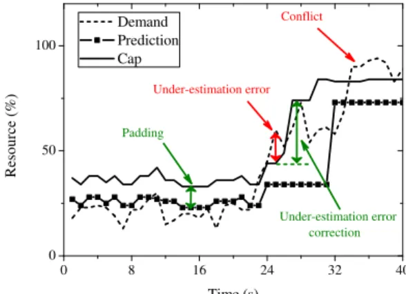
SOCC’11, October 27–28, 2011, Cascais, Portugal. Copyright 2011 ACM 978-1-4503-0976-9/11/10 ...$10.00. 0 8 16 24 32 40 0 50 100 Under-estimation error correction Padding Conflict Under-estimation error R es o u rc e (% ) Time (s) Demand Prediction Cap
Figure 1: Problems and solutions of prediction-driven resource scaling.
provide isolation among uncooperative users. However, statically partitioning the physical resource into virtual machines (VMs) ac-cording to the applications’ peak demands will lead to poor re-source utilization. Overbooking [39] is used to improve the overall resource utilization, and resource capping is applied to achieve per-formance isolation among co-located applications by guaranteeing that no application can consume more resources than those allo-cated to it. However, application resource demand is rarely static, varying as a result of changes in overall workload, the workload mix, and internal application phases and changes. If the resource cap is too low, the application will experience SLO violations. If the resource cap is too high, the cloud service provider has to pay for the wasted resources. To avoid both situations, multi-tenant cloud systems need an elastic resource scaling system to adjust the resource cap dynamically based on application resource demands.
In this paper we present CloudScale, a prediction-driven elas-tic resource scaling system for multi-tenant cloud computing. The goal of our research is to develop an automatic system that can meet the SLO requirements of the applications running inside the cloud with minimum resource and energy cost. In [24], we described our application-agnostic, light-weight online resource demand predic-tor and showed that it can achieve good prediction accuracy for a range of real world applications. When applying the predictor to the resource scaling system, we found that the resource scaling system needs to address a set of new problems in order to reduce SLO violations, illustrated by Figure 1. First, online resource de-mand prediction frequently makes ov and undestimation er-rors. Over-estimations are wasteful, but can be corrected by the on-line resource demand prediction model after it is updated with true application resource demand data. Under-estimations are much
worse since they prevent the system from knowing the true appli-cation resource demand and may cause significant SLO violations. Second, co-located applications will conflict when the available re-sources are insufficient to accommodate all scale-up requirements. CloudScale provides two complementary under-estimation error handling schemes: 1) online adaptive padding and 2) reactive error correction. Our approach is based on the observation that reac-tive error correction alone is often insufficient. When an under-estimation error is detected, an SLO violation has probably already happened. Moreover, there is some delay before the scaling sys-tem can figure out the right resource cap. Thus, it is worthwhile to perform proactive padding to avoid under-estimation errors.
When a scaling conflict happens, we can either reject some scale-up requirements or migrate some applications [14] out of the over-loaded host. Migration is often disruptive, so if the conflict is tran-sient, it is not cost-effective to do this. Moreover, it is often too late to trigger the migration on a conflict since the migration might take a long time to finish when the host is already overloaded. Our approach achieves predictive migration, which can start the tion before the conflict happens to minimize the impact of migra-tion to both migrated and non-migrating applicamigra-tions. CloudScale uses conflict prediction and resolution inference to decide whether a migration should be triggered, which application(s) should be mi-grated, and when the migration should be triggered.
We make the following contributions in this paper:
• We introduce a set of intelligent schemes to reduce SLO vi-olations in a prediction-driven resource scaling system.
• We show how using both adaptive padding and fast estimation error correction minimizes the impact of under-estimation errors with low resource waste.
• We evaluate how well predictive migration resolves scaling conflicts with minimum SLO impact.
• We demonstrate how combining resource scaling with CPU voltage and frequency scaling can save energy without af-fecting application SLOs.
The rest of the paper is organized as follows. Section 2 presents the system design of CloudScale. Section 3 presents the experi-mental results. Section 4 compares our work with related work. Section 5 discusses the limitations and future work. Finally, the paper concludes in Section 6.
2.
CLOUDSCALE DESIGN
In this section, we present the design of CloudScale. First, we provide an overview of our approach. Then, we introduce the sin-gle VM scaling algorithms that can efficiently handle runtime pre-diction errors. Next, we describe how to resolve scaling conflicts. Finally, we describe the integrated VM resource scaling and CPU frequency and voltage scaling for energy saving.
2.1
Overview
CloudScale runs within each host in the cloud system, and is complementary to the resource allocation scheme that handles coarse-grained replicated server capacity scaling [30, 38, 9]. CloudScale is built on top of the Xen virtualization platform. Figure 2 shows the overall architecture of the CloudScale System.
CloudScale uses libxenstat to monitor guest VM’s resource us-age from domain 0. The monitored resource metrics include CPU consumption, memory allocation, network traffic, and disk I/O stat-ics. CloudScale also uses a small memory monitoring daemon
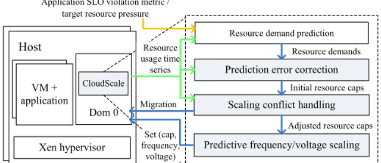
Figure 2: The CloudScale system achitecture.
within each VM to get memory usage statistics (through the /proc interface in Linux). Measurements are taken every 1 second. We use external application SLO monitoring tools [11] to keep track of whether the application SLO is violated. CloudScale currently sup-ports CPU and memory resource scaling. The CPU resource scal-ing is done by adjustscal-ing the CPU cap usscal-ing the Xen credit sched-uler [8] that runs in the non-work-conserving mode (i.e., a domain cannot use more than its share of CPU). The memory resource scal-ing is done usscal-ing Xen’s setMemoryTarget API.
The resource usage time series are fed into an online resource de-mand prediction model to predict the short-term resource dede-mands. CloudScale uses the online resource demand prediction model de-veloped in our previous work [24]. It uses a hybrid approach that employs signature-driven and state-driven prediction algorithms to achieve both high accuracy and low overhead. The model first em-ploys a fast Fourier transform (FFT) to identify repeating patterns called signatures. If a signature is discovered, the prediction model uses it to estimate future resource demands. Otherwise, the pre-diction model employs a discrete-time Markov chain to predict the resource demand in the near future.
The prediction error correction module performs online adap-tive padding that adds a dynamically determined cushion value to the predicted resource demand in order to avoid under-estimation errors. The reactive error correction component detects and cor-rects under-estimation errors that are not prevented by the padding scheme. The result is an initial resource cap for each application VM.
The resource usage time series are also fed into a scaling conflict prediction component. CloudScale decides to trigger VM migra-tions or resolve scaling conflicts locally in the conflict resolution component. The local conflict handling component adjusts the ini-tial resource caps for different VMs according to their priorities when the sum of the initial resource caps exceed the capacity of the host. The migration-based conflict handling component decides when to trigger VM migration and which VM to migrate.
The predictive frequency and voltage scaling module takes the resource cap information to derive the minimum CPU frequency and voltage that can support all the VMs running on the host. The cap adjustment component then calculates the final resource cap values based on the ratio between the new CPU frequency and the old CPU frequency.
In the rest of this section, we will provide details about each major system module.
2.2
Prediction Error Correction
CloudScale incorporates both proactive and reactive approaches to handle under-estimation errors. In this section, we present the online adaptive padding and under-estimation correction schemes.
0 100 200 300 400 0 20 40 60 80 100 C P U u sa g e (% ) Time (s)
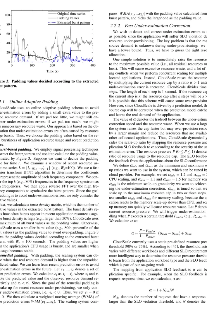
Original time series Padding values Extracted burst pattern
Figure 3: Padding values decided according to the extracted burst pattern.
2.2.1
Online Adaptive Padding
CloudScale uses an online adaptive padding scheme to avoid under-estimation errors by adding a small extra value to the pre-dicted resource demand. If we pad too little, we might still en-counter under-estimation errors; if we pad too much, we might have unnecessary resource waste. Our approach is based on the ob-servation that under-estimation errors are often caused by resource usage bursts. Thus, we choose the padding value based on the re-cent burstiness of application resource usage and rere-cent prediction errors.
Burst-based padding. We employ signal processing techniques to extract the burst pattern and use it to calculate the padding value, illustrated by Figure 3. Suppose we want to decide the padding value for time t. We examine a window of recent resource us-age time series L={lt−Wa, ...,lt−1}(e.g., Wa=100). We use a fast Fourier transform (FFT) algorithm to determine the coefficients that represent the amplitude of each frequency component. We con-sider the top k (e.g., 80%) frequencies in the frequency spectrum as high frequencies. We then apply reverse FFT over the high fre-quency components to synthesize the burst pattern. Since the goal of padding is to avoid under-estimation errors, we only consider the positive values.
Next, we calculate a burst density metric, which is the number of positive values in the extracted burst pattern. The burst density re-flects how often bursts appear in recent application resource usage. If the burst density is high (e.g., larger than 50%), CloudScale uses the maximum of all burst values as the padding value. Otherwise, CloudScale uses a smaller burst value (e.g., 80th percentile of the burst values) as the padding value to avoid over-padding. Figure 3 shows the padding values decided according to the extracted burst pattern, with Wa = 100 seconds. The padding values are higher
when the application’s CPU usage is bursty, and are smaller when the usage becomes stable.
Remedial padding. With padding, the scaling system can ob-serve when the real resource demand is higher than the unpadded predicted value. We can learn from recent prediction errors to avoid under-estimation errors in the future. Let e1, ...,ekdenote a set of
recent prediction errors. We calculate eias xi−x′i, where xiand x′i
denote the predicted value and the observed resource demand re-spectively and xi<x′i. Since the goal of the remedial padding is
to make up for recent resource under-provisioning, we only con-sider under-estimation errors, i.e. ei<0. Thus, we set ei=0 if
ei>0. We then calculate a weighted moving average (WMA) of
those prediction errors W MA(e1, ...ek). The scaling system
com-pares|W MA(e1, ...ek)|with the padding value calculated from the
burst pattern, and picks the larger one as the padding value.
2.2.2
Fast Under-estimation Correction
We wish to detect and correct under-estimation errors as soon as possible since the application will suffer SLO violation during resource under-provisioning. The key problem is that the real re-source demand is unknown during under-provisioning: we only have a lower bound. Thus, we have to guess the right resource allocation.
One simple solution is to immediately raise the resource cap to the maximum possible value (i.e., all residual resources on the host). This will cause excessive resource waste, and a lot of scal-ing conflicts when we perform concurrent scalscal-ing for multiple co-located applications. Instead, CloudScale raises the resource cap by multiplying the current resource cap by a ratioα>1 until the under-estimation error is corrected. CloudScale divides time into steps. The length of each step is 1 second. If the resource cap for the current step is x, the resource cap after k steps will be x×αk.
It is possible that this scheme will cause some over-provisioning. However, since CloudScale is driven by a prediction model, the re-source cap will be corrected when the prediction model catches up and learns the real demand of the application.
The value ofαdenotes the tradeoff between the under-estimation correction speed and the resource waste. When we use a largerα, the system raises the cap faster but may over-provision resources by a larger margin and reduce the resources that are available to other collocated applications. Thus, CloudScale dynamically de-cides the scale-up ratio by mapping the resource pressure and ap-plication SLO feedback toαaccording to the severity of the under-estimation error. The resource pressure P (0≤P≤1) denotes the ratio of resource usage to the resource cap. The SLO feedback is the feedback from the applications about the SLO conformance.
We defineαminandαmaxas the minimum and maximum
scale-up ratios we want to use in the system, which can be tuned by the cloud provider. For example, we setαmin=1.2 andαmax=2 for
CPU scaling, andαmin=1.1 andαmax=1.5 for memory scaling.
αminis the minimum scale-up granularity we want to achieve
dur-ing the under-estimation correction. αmax is tuned so that we can
scale up to the maximum resource cap in two or three steps. We use smallerαminandαmaxfor memory scaling, because the
appli-cation reacts to the memory scale-up slower than CPU, and scaling up memory too quickly will cause resource waste. Let P denote the current resource pressure. We will trigger under-estimation han-dling when P exceeds a certain threshold Punder(e.g., Punder= 0.9).
We calculateαas:
α= P−Punder
1−Punder
·(αmax−αmin) +αmin (1)
CloudScale currently uses a static pre-defined resource pressure threshold (90% or 75%). According to [45], the threshold actually varies with different workloads and different SLO requirements. A more intelligent way to determine the resource pressure threshold is to learn from the application workload type and the SLO feedback, which is part of our on-going work.
The mapping from application SLO feedback toα can be ap-plication specific. For example, when the SLO feedback is the request-response time, we can calculateαas:
α=1+Nvio/N (2)
Nvio denotes the number of requests that have a response time
number of requests during the previous sampling period (e.g., 1 second). For Hadoop applications, the SLO feedback can be job progress scores. We calculateαas 1+ (Pre f−P)/Pre f, where Pre f
denotes the desired progress score derived from the target comple-tion time of the job, and P denotes the current progress score.
When both resource pressure and SLO feedback are available, CloudScale chooses the larger one as the finalα.
2.3
Scaling Conflict Handling
In this section, we describe how we handle concurrent resource scaling for multiple co-located applications. The key issue is to deal with scaling conflicts when the available resources are insuffi-cient to accommodate all scale-up requirements on a host. We first describe how to predict the conflict. Then we introduce the local conflict handling and migration-based conflict handling schemes. Finally we describe the policy of choosing different conflict han-dling approaches.
2.3.1
Conflict Prediction
We can resolve a scaling conflict by either rejecting some ap-plications’ scale-up requirements or employing VM migration to mitigate the conflict. Both approaches will probably cause SLO vi-olations, but we try to minimize these. We use a conflict prediction model to estimate 1) when the conflict will happen, 2) how serious the conflict will be, and 3) how long the conflict will last.
We leverage our resource demand prediction schemes for con-flict prediction, looking further into the future. The scaling system maintains a long-term resource demand prediction model for each VM. Different with the prediction model used by the resource scal-ing system, which uses 1-second prediction interval, the long-term prediction model uses 10-second prediction interval in order to pre-dict further into the future. We use Wb to denote the length of the
look-ahead window of the long-term prediction model (e.g., Wb=
100 seconds). Suppose a host runs K application VMs: m1,...,mK.
Let{ri,t+1, ...ri,t+Wb}denote predicted future resource demands on the mifrom time t+1 to t+Wb. We can then derive the total
re-source demand time series on the host as{∑K
i=1 ri,t+1, ... K ∑ i=1 ri,t+Wb}. By comparing this total resource demand time series with the host resource capacity C, we can estimate when a conflict will happen (i.e., ∑K
i=1
ri,t1>C, t1denotes the conflict start time), how serious the
conflict will be (i.e., the conflict degree:
K
∑
i=1
ri,t1−C), and how long
the conflict will last.
2.3.2
Local conflict handling
If the conflict duration is short and the conflict degree is small, we resolve the scaling conflict locally without invoking expensive migration operations. We define SLO penalty as the financial loss for the cloud provider when applications experience SLO viola-tions, and we use RPi(Resource under-provisioning Penalty) to
de-note the SLO penalty for the application VM micaused by one unit
resource under-provisioning.
Using local conflict handling, we need to consider how to dis-tribute the resource under-provisioning impact among different ap-plications. CloudScale supports both uniform and differentiated local conflict handling. In the uniform scheme, we set the resource cap for each application in proportion to its resource demand. Sup-pose the predicted resource demand for the application VM miis
ri. We set the resource cap for mias(ri/ K
∑
i=1
ri)·C, where C de-notes the total resource capacity on the host. In the differentiated
scheme, CloudScale allocates resources based on application pri-orities or resource under-provisioning penalties (RPi) of different
applications in order to minimize the total penalty. For example, when the VMs have different priorities, CloudScale strives first to satisfy the resource requirements of high-priority applications and only share the under-provisioning impact among low priority appli-cations. CloudScale first ranks all applications according to their priorities, and decides the resource caps of different applications based on the priority rank. If the application’s resource demand can be satisfied by the residual resource, CloudScale will allocate the required resource to the application. Otherwise, CloudScale al-locates the residual resources to all the remaining applications in proportion to their resource demands. We can apply a similar dif-ferentiated allocation scheme when RPiis used to rank different
applications.
We estimate the total SLO penalty for mibased on the conflict
prediction results as
t2
∑
k=t1
RPi·ei,t+k, where t1and t2denote the
con-flict start and end time, and ei,t+kdenotes the undestimation
er-ror at time t+k. We aggregate the SLO penalties of all application VMs to calculate the total resource under-provisioning penalty QRP
using the local conflict handling scheme.
2.3.3
Migration-based conflict handling
If we decide to resolve the scaling conflict using VM migra-tion, we first need to decide when to trigger the migration. We observe that Xen live migration is CPU intensive. Without proper isolation, the migration will cause significant SLO impact to both migrated and non-migrating applications on both source and des-tination hosts. Furthermore, without sufficient CPU, the migration will take a long time to finish, which will lead to a long service degradation time. It is often too late to trigger the migration after the conflict already happened and the host is already overloaded. To address the problem, we use predictive migration, which lever-ages the conflict prediction to trigger migration before the conflict happens. If we want to trigger migration I (e.g., I=70s) before the conflict happens, the migration-based conflict handling mod-ule will check whether any conflict that needs to be resolved using migration will happen after time t+I, where t denotes the current time. If positive, the module will trigger the migration now at time t rather than wait until the conflict happens later after time t+I.
To avoid triggering unnecessary migrations for mis-predicted or transient conflicts, the migration will be triggered only if the con-flict is predicted to last continuously for at least K seconds. The value of K denotes the tradeoff between correct predictions and false alarms, and can be tuned by the cloud provider. Typically we set K=30s, which corresponds to three consecutive predicted con-flicts using a 10-second prediction interval. As a future work, we will make K a function of the migration lead time I and the VM migration time. We may use larger K for longer migration lead time since it will be more likely to have false alarms given a longer migration lead time. For VMs that have longer migration time, we want to avoid unnecessary migrations by using a larger K for lower false alarm rate.
Next, we need to decide which application VMs should be mi-grated. Since modern data centers usually have high speed net-works, the network cost for migration typically is not the major concern. Instead, our scheme focuses on i) migrating as few VMs as possible, and 2) minimizing SLO penalty caused by migrations. Similar to previous work [41], we consider a normalized SLO penalty metric: Zi=MPi·Ti/(w1·cpui+w2·memi), where MPi(Migration
during the migration1; T
idenotes the total migration time for mi;
cpuiand memidenote the normalized CPU and memory utilization
of the application VM micompared to the capacity of the host. The
weights w1and w2denote the importance of the CPU resource or
the memory resource in our decision-making. We can give a higher weight to the bottleneck resource that has lower availability. For example, if the host is CPU-overloaded but has plentiful memory, w1can be much larger than w2so that we will choose a VM with
high CPU consumptions to release sufficient CPU resource. In-tuitively, if the application has low SLO penalty during migration and high resource demands, we want to migrate this application first since the migration imposes low SLO penalty to the migrated application and can release a large amount of resources to resolve conflicts. We sort all application VMs using the normalized SLO penalty metric, and start to migrate the application VMs from the one with the smallest SLO penalty until sufficient resources are re-leased to resolve the conflicts.
Finally, we need to decide which host the selected VM should be migrated to. CloudScale relies on a centralized controller to select the destination host for the migrated application. For example, we can use a greedy algorithm to migrate the VMs to the least loaded host that can accommodate the VM [41], or we can find a suitable host by matching the resource demand signature of the VM with the residual resource signature of the host [23].
We calculate the SLO penalty for migrating mias MPi·Ti. In
our current implementation, we estimate the migration time using a linear function of average memory footprint. The function is de-rived from a few measurement samples using linear regression. We can then aggregate the SLO penalties of all migrated VMs to derive the total migration penalty QMusing the migration-based conflict
handling scheme.
2.3.4
Conflict Resolution Inference
CloudScale currently decides whether to trigger migration by comparing QRPand QM. If QRP≥QM, CloudScale will not
mi-grate any application VM and resolve the scaling conflict using the local conflict handling scheme. Otherwise, CloudScale migrates selected VMs out until sufficient resources are released to resolve the conflict. As a future work, we can also adopt a hybrid ap-proach that combines both local conflict handling and migration-based conflict handling to minimize the total SLO penalty QRP+
QM. We can estimate the total SLO penalty QRP+QMof
migrat-ing different subsets of VMs, and choose the migrated subset that minimizes the total SLO penalty.
The unit SLO penalty values RPiand MPi are application
de-pendent. We assume that these are provided to CloudScale by the user. Typically, batch processing applications (e.g., long run-ning MapReduce jobs) are more tolerant of short periods of ser-vice degradation than time-sensitive interactive applications such as Web transactions.
2.4
Predictive Frequency/Voltage Scaling
CloudScale integrates VM resource scaling with dynamic volt-age and frequency scaling (DVFS) to transform unused resources into energy savings without affecting application SLOs. For ex-ample, if the resource demand prediction models indicate that the total CPU resource demand on a host is 50%, we can then half the CPU frequency and double the resource caps of all application VMs. Thus, we can reduce energy consumption since the CPU runs at a slower speed but the application’s SLO is unaffected. Another
1Although Xen live migration shortens the VM downtime, the
ap-plication may experience a period of high SLO violations due to the memory copy.
way of saving energy is to let the application run as fast as possible and then shutdown the machine. However, the host in the multi-tenant cloud system often runs some interactive foreground jobs that are expected to operate 24x7. Thus, we believe that slowing down the CPU is a more practical solution in this case.
Modern processors often can run at a range of frequencies and voltages and support dynamic frequency/voltage scaling. Suppose the host processor can operate at k different frequencies: f1< ... <
fkand the current frequency is fi. For example, the processor in our
experimental testbed supports 11 different frequencies. We want to slow down the CPU based on the current resource cap information to ensure that application performance is not affected. Let C′and C denote the total CPU demand by all the application VMs and the CPU capacity of the host, respectively. We can then derive the current CPU utilization as C′/C. If the current host does not have a full utilization (i.e., C′/C<1) and the current frequency fiis not the lowest, CloudScale picks the lowest frequency fjthat
meets the condition: fj≥C′/C·fi. If fj< fi, we scale down the
CPU frequency to fj. We then multiply the resource caps for all
application VMs by fi/fj to maintain the application SLOs. To
maintain the accuracy of the resource demand prediction, we also need to scale up the stored resource demand training data by fi/fj
to match the new CPU frequency.
If the processor is not running at the highest frequency, we can increase the CPU speed to try to resolve scaling conflicts. For ex-ample, if the future CPU demand is predicted to be C′,C′>C and the current frequency is fi, we will scale up the CPU frequency to
the slowest one fjamong fi+1, ...fksuch that fj/fi>C′/C. After
we set the CPU frequency to fj, we will scale down the resource
cap rifor each application VM to ri·(fi/fj)to match the new CPU
frequency. After we reach the highest frequency, we will resort to either local conflict handling or migration-based conflict handling, as described in the previous section.
3.
EXPERIMENTAL EVALUATION
We implemented CloudScale on top of the Xen virtualization platform and conducted extensive evaluation studies using the RU-BiS [4] online auction benchmark (PhP version), Hadoop MapRe-duce systems [2, 15], and IBM System S data stream processing system [21]. This section describes our results.
3.1
Experiment setup
Most of our experiments were conducted in the NCSU’s Virtual Computing Lab (VCL) [6]. Each VCL host has a dual-core Xeon 3.00GHz CPU, 4GB memory and 100Mbps network bandwidth, and runs CentOS 5.2 64bit with Xen 3.0.3. The guest VMs also run CentOS 5.2 64bit and have one virtual CPU core (the small-est scheduling unit in Xen hypervisor, similar to the task in Linux kernel).
The integrated VM scaling and DVFS experiments were con-ducted on the Hybrid Green Cloud Computing (HGCC) cluster in our department since VCL hosts are not equipped with power me-ters. Each HGCC node has a quad-core Xeon 2.53GHz processor, 8GB memory and 1Gbps network bandwidth, and runs CentOS 5.5 64 bit with Xen 3.4.3. The processor supports 11 frequency steps between 2.53 and 1.19Ghz. We used Watts Up power meters to get real time power readings from HGCC hosts. The guest VM OS is the same with the VCL host. We use Intel SpeedStep technology to perform DVFS. We run our systems on DVFS enabled Linux 2.6.18 kernel and control the CPU frequency from the host OS using the Linux CPUfreq subsystem.
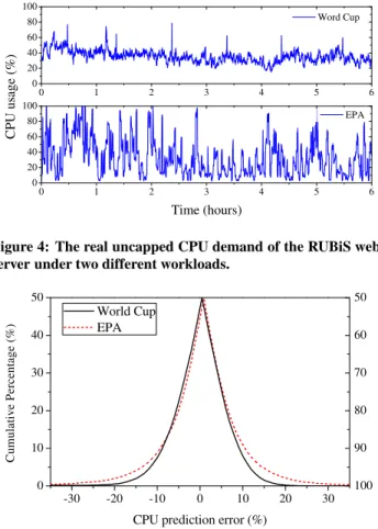
0 1 2 3 4 5 6 0 20 40 60 80 100 EPA Time (hours) 0 1 2 3 4 5 6 0 20 40 60 80 100 Word Cup C P U u sa g e (% )
Figure 4: The real uncapped CPU demand of the RUBiS web-server under two different workloads.
-30 -20 -10 0 10 20 30 0 10 20 30 40 50 C u m u la ti v e P e rc e n ta g e ( % )
CPU prediction error (%) World Cup EPA 100 90 80 70 60 50
Figure 5: Folded cumulative distribution of CPU resource de-mand prediction errors for two different workloads. The left half is a normal CDF using the y-axis scale on the left; the right half, using the scale on the right, is the reflected upper half of the CDF.
run all guest VMs on another core. CloudScale runs within Domain 0.
CloudScale performs fine-grained monitoring by frequently sam-pling all resource metrics and repeatedly updates the resource de-mand prediction model using a number of recent resource usage samples. The resource scaling period, the sampling period, pre-diction model update period, and training data size are all tunable parameters. For CPU scaling, CloudScale uses a 1 second scaling and sampling period, 10 second prediction model update period, 100 recent resource usage samples as training data for the short-term resource demand prediction model, and 2000 recent resource usage samples as training data for the long-term conflict prediction model. For memory scaling, the default setup is the same as CPU scaling except that the scaling period is 10 seconds, and the training data set for short-term resource demand prediction model contains 1000 recent resource usage samples. We found that the default set-tings work well for all of the applications used in our experiments. A service provider can either rely on the application itself or an external tool [11] to keep track of whether the application SLO is violated. In our experiments with RUBiS and IBM System S, we adopted the latter approach, using the workload generator to track the response time of the HTTP requests it made or the processing day of each stream data tuple. In RUBiS, the SLO violation rate is the fraction of requests that have response time larger than the pre-defined SLO threshold (200 ms) during each experiment run.
Scheme PredictionError Correction OnlineAdaptive Padding
Correction Resource pressure none
Dynamic padding none Dynamic
Padding-X% none Constant X%
CloudScale RP Resource pressure Dynamic CloudScale RP + SLO Resource pressure
+ SLO feedback Dynamic Table 1: Configurations of different schemes.
In System S, the SLO violation rate is the fraction of data tuples that have processing delay larger than the pre-defined SLO thresh-old (20 ms). In Hadoop experiments, we used the progress score provided by the Hadoop API as the SLO feedback, and transform the target job completion time into the desired progress score. The SLO violation rate is sampled every second in RUBiS and System S. In Hadoop, since calling the Hadoop API to get the progress score will take a long time (> 1 minute) to return, we try to get the updated progress score as fast as possible by calling the API again immediately after getting the returned value.
To evaluate CloudScale under workloads with realistic time vari-ations, we used per-minute workload intensity observed in real-world Web traces [5] to modulate the request rate of the RUBiS benchmark and the input data rate to the System S stream process-ing system. We constructed two workload time series: 1) the re-quest rate observed in each minute of the six-hour World Cup 98 web server trace starting at 1998-05-05:00.00; and 2) the request rate observed in each minute of the six-hour EPA web server trace starting at 1995-08-29:23.53.
For comparison, we also implemented a set of alternative schemes and several variations of the CloudScale system, summarized in Ta-ble 1: 1) Correction: the scaling system performs resource pressure triggered prediction error correction only; 2) Dynamic padding: the scaling system performs dynamic padding only; 3) Padding-x%: the scaling system performs a constant percentage padding by adding x% predicted value; 4) CloudScale RP: the scaling system performs both dynamic padding and scaling error correction, and the scaling error correction is only triggered by resource pressure; and 5) CloudScale RP+SLO: the scaling system performs both dy-namic padding and scaling error correction, and the scaling error correction is triggered by both resource pressure and SLO feed-back.
3.2
Results
Figure 4 shows the real CPU demand (the CPU usage achieved with no resource caps) for the RUBiS Web server under two test workload patterns. Both workloads have fluctuating CPU demands. We focus on CPU resource scaling in RUBiS experiments since it appears to be the bottleneck in this application.
Figure 5 shows the accuracy of online resource demand pre-diction using folded cumulative distributions. The results show that the resource demand prediction makes less than 5% significant under-estimation or over-estimation errors (i.e.,|e|>10%) for the World Cup workload and about 10% significant under-estimation or over-estimation errors for the EPA workload.
We conducted experiments for both single VM and multiple VMs. For single VM case, the VM hosts a RUBiS web server. For the multi-VM case, there were two VMs running on the same physical host, each hosting a RUBiS Web server driven by the World Cup workload and the EPA workload respectively. The database servers run on different physical hosts. During the multi-VM scaling ex-periment, all the VMs have equal priority.
World Cup EPA Both 0 5 10 S L O v io la ti o n r at e (% )
World Cup EPA Both
0 50 100 M ea n r es p o n se t im e (m s)
World Cup EPA Both
0 100 200 300 T o ta l C P U a ll o ca ti o n s (m in )
Correction Dynamic padding CloudScale RP CloudScale RP+SLO
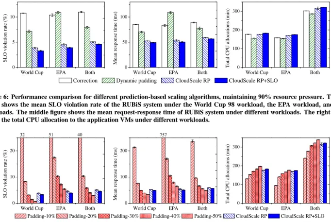
Figure 6: Performance comparison for different prediction-based scaling algorithms, maintaining 90% resource pressure. The left figure shows the mean SLO violation rate of the RUBiS system under the World Cup 98 workload, the EPA workload, and both workloads. The middle figure shows the mean request-response time of RUBiS system under different workloads. The right figure shows the total CPU allocation to the application VMs under different workloads.
World Cup EPA Both
0 10 20 40 51 32 S L O v io la ti o n r at e (% )
World Cup EPA Both
0 100 200 757 M ea n r es p o n se t im e (m s)
World Cup EPA Both
0 100 200 300 T o ta l C P U a ll o ca ti o n s (m in )
Padding-10% Padding-20% Padding-30% Padding-40% Padding-50% CloudScale RP CloudScale RP+SLO Figure 7: Performance comparison for CloudScale and constant padding algorithms, maintaining 90% resource pressure. The left figure shows the mean SLO violation rate of the RUBiS system under the World Cup 98 workload, the EPA workload, and both workloads. The middle figure shows the mean request-response time of RUBiS system under different workloads. The right figure shows the total CPU allocation to the application VMs under different workloads.
Figure 6 and Figure 7 show the performance and total CPU al-locations of different scaling schemes. In these experiments, the resource pressure threshold to trigger under-estimation error cor-rection is set at 90% and the SLO triggering threshold is set at 5% requests experience SLO violation (i.e., response time>200ms). The total CPU allocation is calculated based on the resource cap set by different schemes. Each experiment is repeated three times and we report both mean and standard deviations.
Figure 6 shows that CloudScale can achieve lower SLO viola-tion rate and smaller response time than other schemes. Both reac-tive correction and dynamic padding when used alone can partially alleviate the problem. But dynamic padding works better for the World Cup workload, while the reactive correction works better for the EPA workload, because the EPA workload shows more fluctu-ations and reactive correction becomes more important. We also observe that runtime SLO feedback is helpful, but not vital, for CloudScale to reduce SLO violations. CloudScale also achieves better performance than other schemes in the multi-VM concurrent scaling case.
Figure 7 shows the performance comparison between Cloud-Scale with different constant padding schemes. The results show that if we pad too little (e.g., padding-10%), we have high SLO vi-olations and if we pad too much (e.g., padding-50%), we have low SLO violation rate but at high resource cost. When the resource al-location reaches a certain threshold, more padding does not reduce the response time and SLO violation rate much. More importantly, it is hard to decide how much to pad in advance if we use constant padding schemes. In contrast, CloudScale does not need to specify
the padding percentage, and is able to adjust the padding during runtime automatically.
We learned from our experiments that the prediction-only scheme performs poorly without under-estimation correction and padding, which is not shown in the figures. The reason is that the prediction model cannot get the real resource demand when under-estimation error happens, and can only learn the distorted demand values. Since the application cannot consume more resources than the re-source cap, once the rere-source cap is pushed down, it will not be raised anymore. In this case, the scaling system will predict and al-locate less and less resources, and the application will suffer from severe resource under-provisioning.
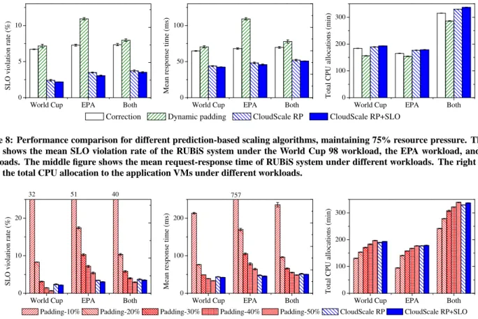
Figure 8 and Figure 9 shows the results of the same set of ex-periments but with the resource pressure threshold set at 75%. The SLO violation rates are consistently lower for all algorithms when compared to the 90% resource pressure threshold cases. Note that CloudScale RP+SLO achieves much better performance in this case. That is because CloudScale RP+SLO considers both resource pres-sure and SLO feedback. Moreover, since the SLO triggering thresh-old is set at 5%, and we derive the scale-up ratioαusing equation 2, α derived from SLO feedback is typically very small and the resource pressure feedback becomes the dominant factor in trig-gering scaling error corrections. We can see that CloudScale still achieves the best application performance with low resource cost. The benefit of CloudScale is more significant for EPA trace, achiev-ing much lower SLO violations and smaller response time than the generous constant padding scheme “padding-50%” but with a sim-ilar resource cost. The reason is that the EPA trace is very bursty
World Cup EPA Both 0 5 10 S L O v io la ti o n r at e (% )
World Cup EPA Both
0 50 100 M ea n r es p o n se t im e (m s)
World Cup EPA Both
0 100 200 300 T o ta l C P U a ll o ca ti o n s (m in )
Correction Dynamic padding CloudScale RP CloudScale RP+SLO
Figure 8: Performance comparison for different prediction-based scaling algorithms, maintaining 75% resource pressure. The left figure shows the mean SLO violation rate of the RUBiS system under the World Cup 98 workload, the EPA workload, and both workloads. The middle figure shows the mean request-response time of RUBiS system under different workloads. The right figure shows the total CPU allocation to the application VMs under different workloads.
World Cup EPA Both
0 10 20 S L O v io la ti o n r at e (% )
World Cup EPA Both
0 100 200 M ea n r es p o n se t im e (m s)
World Cup EPA Both
0 100 200 300
Padding-10% Padding-20% Padding-30% Padding-40% Padding-50% CloudScale RP CloudScale RP+SLO
T o ta l C P U a ll o ca ti o n s (m in ) 40 51 32 757
Figure 9: Performance comparison for CloudScale and constant padding algorithms, maintaining 75% resource pressure. The left figure shows the mean SLO violation rate of the RUBiS system under the World Cup 98 workload, the EPA workload, and both workloads. The middle figure shows the mean request-response time of RUBiS system under different workloads. The right figure shows the total CPU allocation to the application VMs under different workloads.
and intelligent handling of under-estimation plays a critical role in this case.
Figure 10 shows the energy saving effectiveness of the predic-tive CPU scaling. We repeated the same RUBiS experiments as the CloudScale RP+SLO scheme on the HGCC cluster, and set the re-source pressure threshold as 90%. We ran each experiment for 6 hours and measured the total energy consumption for both Cloud-Scale without DVFS and with DVFS. Without DVFS, the CPU runs at the maximum frequency. The idle energy consumption is mea-sured when the host is idle and stays at its lowest power state. The workload energy consumption is derived by subtracting the idle en-ergy consumption from the total enen-ergy consumption. The results show that CloudScale with DVFS enabled (CloudScale DVFS) can save 8-10% total energy consumption, and 39-71% workload en-ergy consumption with little impact to the application performance and SLO conformance. We also observe that compared to the work-load energy consumptions, the idle energy consumptions are dom-inating in all cases. This is because all HGCC hosts are powerful quad-core machines and each experiment run only uses two cores: one core for the application VM and one core for Domain 0. We be-lieve that CloudScale DVFS can achieve higher total energy saving when more cores are utilized.
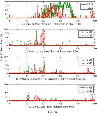
We now evaluate our conflict handling schemes. We run two RUBiS web server VMs on the same host, and maintain a 75% re-source pressure with dynamic padding. The local conflict handling uses the uniform handling policy that treats the two VMs uniformly. The memory size of VM1 is 1GB, and the memory size of VM2 is
2GB, so the migration time of VM2 is much longer than VM1. We sample the SLO violation rate every second for both VMs, and cal-culate the total time that the application experiences different SLO violation rates. Figure 11(a) shows the SLO violation time under the local conflict handling scheme. We can see that when conflict happens, both VMs suffer from high SLO violation rates for a long period of time. The total time that both VMs experience SLO viola-tions adds up to 351 seconds. We then evaluate the migration-based conflict handling schemes. We first test with the reactive migration scheme where the scaling system triggers the live migration to mi-grate VM2 out after it detects a sustained scaling conflict using the algorithm proposed in [41]. In Figure 11(b), we can see that the migration reduces the SLO violation time significantly. The total time of having SLO violations becomes 92 seconds. However, the live migration still takes a long time to finish when the system is overloaded and both non-migrating and migrated VMs experience significant SLO violations during the migration. We then enable the CloudScale’s VM selection algorithm that selects the migrated VM based on the normalized SLO penalty metric. In this experiment, we used equal weights for CPU and memory. We set RP1=RP2=1
and MP1=MP2=8 (RP1and RP2denote the unit resource
under-provisioning penalties for VM1 and VM2 respectively; MP1and
MP2denote the unit migration penalty for VM1 and VM2
respec-tively). We tried different ratios between MP and RP, and find that setting MP/RP=8 provides a reasonable tradeoff between local conflict resolving and migration. The migration time is estimated using the regression-derived function shown by Figure 14. In this
World Cup EPA Both 0.00 0.20 0.40 0.60 T o ta l en er g y c o n su m p ti o n ( K W h )
Workload energy consumption - CloudScale Workload energy consumption - CloudScale DVFS Idle power
(a) Total energy consumption
World Cup EPA Both
0 30 60 M ea n r es p o n se t im e (m s) CloudScale CloudScale DVFS
(b) Mean response time.
World Cup EPA Both
0 4 8 S L O v io la ti o n r at e (% ) CloudScale CloudScale DVFS
(c) SLO violation rate.
Figure 10: Effect on energy consumption and applica-tion performance of RUBiS applicaapplica-tion using predictive fre-quency/voltage scaling (maintaining 90% resource pressure).
case, the system selects VM1 instead of VM2 to migrate out. From Figure 11(c) we can see that although the total SLO violation dura-tion is similar to the previous case (90 seconds), the SLO violadura-tion rates are much smaller.
We then repeat the same experiment using CloudScale’s conflict handling scheme. The predictive migration triggers the migration of VM1 about 70 seconds before the conflict happens. From Fig-ure 11(d) we can see that the live migration can finish in a short pe-riod of time and both VMs experience shorter SLO violation time. The total SLO violation duration is reduced to 60 seconds.
Figure 12 shows the cumulative percentage of continuous SLO violation duration under different SLO violation rates. When re-solving the conflict locally, more than 10% of the violation dura-tions are longer than 5 seconds. Using reactive migration, less than 5% of the SLO violation durations are more than 5 seconds, but the application can still experience up to 19 seconds of continuous SLO violations. After enabling our VM selection algorithm, the maximum continuous SLO violation time becomes 4 seconds. In contrast, when using CloudScale’s conflict handling scheme, the continuous SLO violation durations are always less than 2 seconds, and 90% of the continuous SLO violation durations are only 1 sec-ond.
Figure 13 shows the cumulative percentage of SLO violation
0 100 200 300 400 500 0 25 50 75 100
(d) CloudScale (Total violation time: 60s) (c) Reactive migration + VM selection (Total violation time: 90s)
(b) Reactive migration (Total violation time: 92s)
VM1 VM2
(a) Local conflict resolving (Total violation time: 351s)
0 100 200 300 400 500 0 25 50 75 100 S L O V io la ti o n R at e (% ) VM1 VM2 0 100 200 300 400 500 0 25 50 75 100 Time (s) VM1 VM2 0 100 200 300 400 500 0 25 50 75 100 VM1 VM2
Figure 11: Time series of SLO violation rate for different scal-ing conflict resolvscal-ing schemes.
rates using different scaling conflict schemes. When using Cloud-Scale’s conflict handling scheme, the application does not experi-ence any SLO violation for 94% of the time, and the SLO violation rate is less than 20% for 99% of the time. All of the other schemes incur higher SLO violation rates than CloudScale.
To measure the accuracy of our conflict prediction algorithms, we used six hours of CPU demand traces for two RUBiS web servers used in previous experiments for different scaling schemes. We first mark the start time of all significant conflicts, then use our conflict prediction algorithms to predict the conflict within differ-ent time windows. By comparing predicted conflicts with true con-flicts, we calculate the number of true positive predictions (Ntp): the
conflicts that are predicted correctly; the number of false-negative predictions (Nfn): the conflicts that were not predicted; the
num-ber of false-positive predictions (Nfp): the predicted conflicts that
did not happen; and the number of true-negative predictions (Ntn):
the non-conflicts that are predicted correctly. The true positive rate AT and false alarm rate AF are defined in a standard way as
AT=Ntp/(Ntp+Nfn); AF=Nfp/(Nfp+Ntn). Figure 15 shows the
true positive and false positive rate of our conflict prediction algo-rithms under different migration lead time requirements. As ex-pected, the prediction accuracy decreases with a longer migration lead time (i.e., triggering migration earlier). However, since predic-tive migration is triggered before conflict happens, the SLO impact of false alarms is small. We plan to further improve the accuracy of the conflict prediction algorithm in our future work.
We then apply the scaling system to a Hadoop MapReduce ap-plication. Unlike RUBiS, the Hadoop application is memory in-tensive, so we focus on memory scaling in this set of experiments. We used the Word Count and Grep MapReduce sample applica-tions. One VM holds all the map tasks while another VM holds all the reduce tasks. The number of slots for map tasks or reduce tasks is set to 2 on both nodes. Figure 16 shows the real memory
1 5 10 15 20 40 60 80 100 C u m u la ti v e P er ce n ta g e (% )
Continuous SLO violation duration (s) CloudScale (Total: 11s)
Reactive migration + VM selection (Total: 23s) Reactive migration (Total: 38s)
Local conflict resolving (Total: 238s)
Figure 12: CDF of continuous SLO violation duration (when SLO violation rate is larger than 20%) comparison among dif-ferent scaling conflict resolving schemes for the RUBiS system.
0 20 40 60 80 100 60 70 80 90 100 C u m u la ti v e P er ce n ta g e (% )
SLO Violation Rate (%) CloudScale
Reactive migration + VM selection Reactive migration
Local conflict resolving
Figure 13: CDF of SLO violation rate comparison among dif-ferent scaling conflict resolving schemes for the RUBiS system.
demand (the memory footprint achieved with no memory cap) of the VM hosting map tasks. We can see that the memory footprint of the VM fluctuates a lot. The peak memory footprint of word count is 591MB, and the peak memory footprint of grep is 579MB. Without scaling, we have to perform memory allocation based on the maximum memory footprint, which will cause memory waste. Moreover, it is hard to get the maximum memory footprint in ad-vance. We apply predictive memory scaling on Hadoop. Figure 17 shows the prediction accuracy of memory scaling. As with CPU, CloudScale can achieve good prediction accuracy for memory.
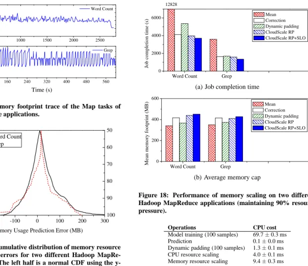
Figure 18 shows the job completion time and average memory caps of different scaling schemes. Since the progress score of map tasks is more accurate than that of reduce tasks, we only performed memory scaling on the map VM and the reduce VM is always given sufficient memory. The resource pressure threshold is set as 90%. We observe that CloudScale can achieve the shortest job comple-tion time with low memory cap. We use “mean” to denote the static memory allocation scheme that allocates a fixed amount of memory based on the average memory footprint in the real mem-ory demand trace. The results show that this static scheme works poorly, which significantly increases the job completion time: the system spends a long time on swapping memory pages when more memory is needed. In contrast, CloudScale does not know the exact memory demand in advance, but still achieves better performance. The effect of progress score feedback is not significant. As
men-1000 1500 2000 16 20 24 28 32 M ig ra ti o n t im e (s ) Memory size (MB) Migration time model
Sample data for calculating the regression model Real data observed in experiments
Figure 14: Migration time estimation model. The model is a linear regression of the sample data we got by measuring the migration time of the VMs with different memory sizes. We also put the real data that we observed in the experiments to show the accuracy of the model.
7 14 21 28 35 42 49 56 63 70 0 20 40 60 80 100 P re d ic ti o n a cc u ra cy ( % ) Lead time (s)
True positive rate False positive rate
Figure 15: Conflict prediction accuracy under different migra-tion lead time requirements.
tioned before, calling the Hadoop API to get the progress score will take a long time (10 to 60 seconds) to return, especially when the node is busy with memory page swapping. When the application is suffering from resource under-provisioning, CloudScale cannot trigger under-estimation handling in time because it cannot get the SLO feedback immediately.
We now evaluate CloudScale on IBM System S, a production data stream processing system. We run one of the sample applica-tions provided by System S. It is a tax calculation application that takes commodity records including commodity name, seller, price, quantity and state as the input stream tuples and calculates the fi-nal price for each tuple based on the tax rates of different states. We used the sample data provided by the System S. To emulate dynamic data arrivals, we used the World Cup and EPA workload to regulate the input data rate. The average input rate is about 1 million data tuples per second. The application consists of 7 dis-tributed processing elements (PEs). We run each PE within one VM. All VMs are deployed on different hosts. Since CloudScale focuses on resource scaling within single host, we perform CPU scaling on one of the PEs and always give sufficient resources to the other PEs. We set the resource pressure to 90%, and measure the
0 500 1000 1500 2000 2500 0 200 400 600 800 Word Count M em o ry f o o tp ri n t (M B ) 0 80 160 240 320 400 480 560 0 200 400 600 Time (s) Grep
Figure 16: The memory footprint trace of the Map tasks of Hadoop MapReduce applications.
-300 -200 -100 0 100 200 300 0 10 20 30 40 50 C u m u la ti v e P er ce n ta g e (% )
Memory Usage Prediction Error (MB) Word Count Grep 100 90 80 70 60 50
Figure 17: Folded cumulative distribution of memory resource demand prediction errors for two different Hadoop MapRe-duce applications. The left half is a normal CDF using the y-axis scale on the left; the right half, using the scale on the right, is the reflected upper half of the CDF.
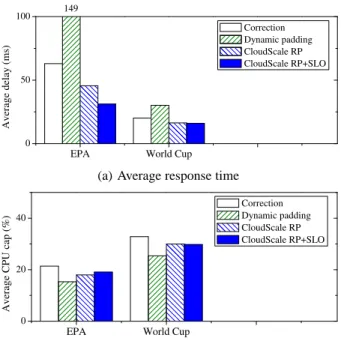
per-tuple processing delay. Figure 19 shows the performance and average CPU cap achieved by different scaling algorithms. The results show that CloudScale can achieve much lower processing delay than other prediction-based scaling schemes with low CPU caps.
We now evaluate the overhead of the CloudScale system. Ta-ble 2 shows the CPU overhead of all the key operations in Cloud-Scale. The results show that CloudScale is light-weight for all op-erations. In our experiment environment, running CloudScale only consumes about 2% CPU resource in Domain 0. Thus, we believe that CloudScale is suitable for large-scale cloud systems.
4.
RELATED WORK
Existing production cloud system scaling techniques such as Ama-zon Auto Scaling [1] is not fully automatic, which depend on the user to define the conditions for scaling up or down resources. However, it is often difficult for the user to figure out the proper scaling conditions, especially when the application will be executed on a third-party virtualized cloud computing infrastructure.
Several projects [30, 38, 9] studied coarse-grained capacity scal-ing scheme by dynamically addscal-ing or releasscal-ing server nodes in a particular system tier. The tier scaling schemes focus on determin-ing how many server hosts are needed in each tier usdetermin-ing queuedetermin-ing theory [38], machine learning [9], or control theory [30], and how to rebalance workload among replicated server instances. In
com-Word Count Grep 0 2000 4000 6000 Jo b c o m p le ti o n t im e (s ) Mean Correction Dynamic padding CloudScale RP CloudScale RP+SLO 12828
(a) Job completion time
Word Count Grep 0 200 400 600 M ea n m em o ry f o o tp ri n t (M B ) Mean Correction Dynamic padding CloudScale RP CloudScale RP+SLO
(b) Average memory cap
Figure 18: Performance of memory scaling on two different Hadoop MapReduce applications (maintaining 90% resource pressure).
Operations CPU cost
Model training (100 samples) 69.7±0.3 ms
Prediction 0.1±0.0 ms
Dynamic padding (100 samples) 1.3±0.1 ms CPU resource scaling 4.0±0.1 ms Memory resource scaling 9.4±0.3 ms
Table 2: Mean and standard deviation of CPU execution costs for all core operations in CloudScale, averaged over 300 opera-tions on Xeon 3.0GHz CPU.
parison, our work focuses on fine-grained VM-level resource scal-ing, which can be used on each server node to adaptively adjust resource allocation to different VMs for reducing resource and en-ergy cost. Our scaling scheme is complementary to the host-level tier scaling scheme.
Previous work [44, 29, 31, 36, 32] has extensively studied apply-ing control theory to achieve adaptive fine-grained resource alloca-tions based on SLO conformance feedback. However, those ap-proaches often have parameters that need to be specified or tuned offline, and need some time to converge to the optimal (or near-optimal) decisions. In contrast, CloudScale does not require any offline tuning and can achieve elastic resource allocation without assuming any prior knowledge about applications.
Our work is closely related to trace-driven resource allocation schemes. Rolia et al. [33] proposed a dynamic resource alloca-tion scheme by multiplying estimated resource usage with a burst factor that is derived offline based on different QoS levels. In con-trast, our scheme performs online burst pattern extraction and uses the burst pattern to dynamically decide the padding value. Chan-dra et al. [12] proposed workload prediction using auto-regression and histogram based methods. Gmach et al. [22] used a Fourier transform-based scheme to perform offline extraction of long-term cyclic workload patterns. Our previous system PRESS [24]
pro-EPA World Cup 0 50 100 A v er ag e d el ay ( m s) Correction Dynamic padding CloudScale RP CloudScale RP+SLO 149
(a) Average response time
EPA World Cup
0 20 40 A v er ag e C P U c ap ( % ) Correction Dynamic padding CloudScale RP CloudScale RP+SLO
(b) Average CPU cap
Figure 19: Performance of CPU scaling on IBM System S (maintaining 90% resource pressure).
vides a hybrid resource demand prediction scheme that can achieve both high accuracy and low overhead. In contrast, this work fo-cuses on efficiently handling prediction errors and concurrent scal-ing conflicts to achieve elastic resource scalscal-ing for multi-tenant cloud systems.
Previous work has proposed model-driven resource allocation schemes. Those approaches use statistical learning methods [34, 37, 20, 35] or queueing theory [17] to build models that allow the system to predict the impact of different resource allocation policies on the application performance. However, those models need to be built with non-trivial overhead and calibrated in ad-vance. Moreover, the resource allocation system needs to assume certain prior knowledge about the application and the running plat-form (e.g., input data size, cache size, processor speed), which often is impractical in the cloud system. In contrast, CloudScale is completely application and platform agnostic, which makes it more suitable for cloud computing infrastructures that often host third-party applications. Other work has used offline or online profiling [39, 40, 43, 25] to experimentally derive application re-source requirements using benchmark or real application work-loads. However, profiling needs extra machines and may take a long time to derive resource requirements. Our experiments using the perfect prediction scheme also show that profiling often does not work well for fine-grained resource control since a tiny shift in time will cause significant performance impact.
Virtual machine migration [14] has been widely used for dy-namic resource provisioning. Sandpiper [41] is a system that au-tomates the task of monitoring and detecting hotspots, determining a new mapping of physical to virtual resources, and initiating nec-essary migrations. It uses both black-box and gray-box approach to detect hotspots and determine resource provisioning. The mi-gration is triggered in Sandpiper when a certain metric exceeds some threshold for a sustained time and the next predicted value also exceeds the threshold. In comparison, our work leverages live VM migrations to resolve significant scaling conflicts. Our
scheme leverages long-term prediction to trigger migration before conflict happens and makes migration decisions based on the im-pact of migration to application SLOs. Entropy [27] is a resource manager for homogeneous clusters, which performs dynamic con-solidation based on constraint programming and takes migration overhead into account. Entropy assumes that the resource demand is known in advance. In contrast, our work focuses on addressing the challenge in predicting the resource demand and the impact of migration.
Although initial work [19, 42] on power saving focused on mo-bile devices, it has become increasingly important to consider en-ergy saving while managing large-scale hosting centers. Muse [13] is one pioneering work that integrates energy management into comprehensive resource management. It proposed an economic ap-proach to adaptive resource provisioning and an on-power capacity scaling system that can adaptively turn on/off some hosts based on the workload needs. ACES [26] is an automatic controller for energy-aware server provisioning that provisions servers to meet workload demand while minimizing the energy, maintenance and reliability cost. ACES tries to balance the tradeoff between en-ergy savings and reliability impact due to on-off cycles. It uses regression analysis to predict workload demand in the near future, and has a model to quantify the reliability impact in terms of its dollar cost. ACES focuses on using low power states (off, sleep, hibernate) instead of DVFS. In comparison, our work focuses on integrating fine-grained resource scaling and DVFS to achieve en-ergy saving. Our approach is complementary to Muse and ACES system, which can be particularly useful for multi-tenant cloud sys-tems when host shutdown is not an option. DVFS has been shown to be effective for reducing power consumption of large-scale com-puter systems [28]. Previous work (e.g., [16]) focuses on OS level task characterization and uses learning algorithms to estimate the best suited voltage and frequency setting. Fan et al. [18] used simulation to calculate the potential of power and energy saving in large scale systems using power management techniques based on DVFS. It considers triggering DVFS according to different CPU utilization thresholds. In comparison, our scheme integrates DVFS with VM scaling and leverages predicted resource caps to derive the proper frequency/voltage setting.
5.
FUTURE WORK
Although demonstrated efficient in experiments, CloudScale has several limitations which we plan to address in our future work.
CloudScale currently uses a pre-defined resource pressure thresh-old. Although the resource pressure maintenance and SLO feed-back handling can work together, CloudScale currently does not adjust resource pressure threshold dynamically according to the workload type or SLO feedback. However, different types of appli-cations might need varying resource pressure thresholds for trigger-ing the under-estimation handltrigger-ing. For example, an interactive ap-plication typically needs to avoid high resource pressure for main-taining sufficient resources to serve any requests as soon as they arrive. In contrast, for batch jobs, we can afford to maintain a tight resource pressure to achieve high resource utilization without sig-nificant SLO violations. To make CloudScale more intelligent, we can automatically tune the resource pressure threshold based on some general knowledge about the application (e.g. interactive v.s. batch jobs) or coarse-grained SLO feedback.
CloudScale can scale on different metrics independently, but does not coordinate the scaling operations on them. It is a non-trivial re-search task to efficiently handle potential interference between dif-ferent resource scaling operations. The problem is that adjusting the allocation of one resource type can affect the usage of another
type of resource, which might introduce more dynamics into the system and cause more prediction errors. To address the problem, we plan to investigate multi-metric prediction model that can pre-dict multiple metrics together and scale them concurrently.
Similar to multi-metric scaling, it is also challenging to handle multi-tier application scaling, in which different tiers have inter-dependency and scaling on one tier can affect the others. We can integrate CloudScale with host-level scaling techniques [30, 38, 9] to handle multi-tier application scaling efficiently by predicting the resource demand of different tiers at the same time and coordinat-ing the scalcoordinat-ing operation on different hosts.
CloudScale performs long-term conflict prediction by extracting the repeating pattern in the resource usage trace. When the repeat-ing pattern is not found, CloudScale relies on multi-step Markov prediction algorithms for long-term predictions. However, multi-step Markov prediction has limited prediction accuracy since the correlation between the resource prediction model and the actual resource demand becomes weaker as we look further into the fu-ture. We are investigating other long-term prediction models to bet-ter handle the case when no periodic patbet-tern is found in the training data.
CloudScale currently works in the capping mode, which isolates co-located applications by ensuring that the application cannot con-sume more resources than those allocated to it. Xen credit sched-uler also supports a weight mode: assigning each VM a weight which indicates the relative CPU share of the VM. CloudScale can be easily extended to support weight mode by adjusting the weight of the VMs dynamically based on the resource demand prediction. In contrast to the capping mode, VMs can consume residual CPU resources out of their shares in weight mode. However, when re-source contention happens, weight mode cannot provide perfor-mance isolation, and it is impossible to know the real demand of the collocated VMs since their resource usages are affected by each other. As a future work, we will leverage our conflict prediction to dynamically switch between capping mode and weight mode. When there is no conflict, CloudScale can work in weight mode to improve the resource utilization. When there are conflicts, Cloud-Scale can work in capping mode to ensure performance isolation.
6.
CONCLUSION
In this paper, we presented CloudScale, an automatic elastic re-source scaling system for multi-tenant cloud computing infrastruc-tures. CloudScale consists of three key components: 1) combin-ing online resource demand prediction and efficient prediction er-ror handling to meet application SLOs with minimum resource cost; 2) supporting multi-VM concurrent scaling with conflict pre-diction and predicted migration to resolve scaling conflicts with minimum SLO impact; and 3) integrating VM resource scaling with dynamic voltage and frequency scaling (DVFS) to save en-ergy without affecting application SLOs. We have implemented CloudScale on top of the Xen virtualization platform and conducted extensive experiments using the RUBiS benchmark driven by real Web server traces, Hadoop MapReduce systems, and a commer-cial stream processing system. The experimental results show that CloudScale can achieve much better SLO conformance than other alternative schemes with low resource cost. CloudScale can re-solve scaling conflicts with up to 83% less SLO violation time than other schemes. CloudScale can save 8-10% total energy consump-tion, and 39-71% workload energy consumption with little impact to the application performance and SLO conformance. CloudScale is light-weight and application-agnostic, which makes it suitable for large-scale cloud systems.
7.
ACKNOWLEDGEMENT
This work was sponsored in part by NSF CNS0915567 grant, NSF CNS0915861 grant, U.S. Army Research Office (ARO) un-der grant W911NF-10-1-0273, and Google Research Awards. Any opinions expressed in this paper are those of the authors and do not necessarily reflect the views of the NSF, ARO, or U.S. Govern-ment. The authors thank the anonymous reviewers for their insight-ful comments.
8.
REFERENCES
[1] Amazon Elastic Compute Cloud. http://aws.amazon.com/ec2/.
[2] Apache Hadoop System. http://hadoop.apache.org/core/. [3] KVM (Kernel-based Virtual Machine).
http://www.linux-kvm.org/page/Main_Page. [4] RUBiS Online Auction System. http://rubis.ow2.org/. [5] The IRCache Project. http://www.ircache.net/. [6] Virtual Computing Lab. http://vcl.ncsu.edu/. [7] VMware Virtualization Technology.
http://www.vmware.com/. [8] Xen Credit Scheduler.
http://wiki.xensource.com/xenwiki/CreditScheduler. [9] M. Armbrust, A. Fox, D. A. Patterson, N. Lanham,
B. Trushkowsky, J. Trutna, and H. Oh. Scads:
Scale-independent storage for social computing applications. In Proc. CIDR, 2009.
[10] P. Barham and et al. Xen and the art of virtualization. In Proc. SOSP, 2003.
[11] D. Breitgand, M. B.-Yehuda, M. Factor, H. Kolodner, V. Kravtsov, and D. Pelleg. NAP: a building block for remediating performance bottlenecks via black box network analysis. In Proc. ICAC, 2009.
[12] A. Chandra, W. Gong, and P. Shenoy. Dynamic resource allocation for shared data centers using online
measurements. In Proc. IWQoS, 2004.
[13] J. Chase, D. Anderson, P. N. Thakar, and A. M. Vahdat. Managing energy and server resources in hosting centers. In Proc. SOSP, 2001.
[14] C. Clark, K. Fraser, S. Hand, J. G. Hansen, E. Jul, C. Limpach, I. Pratt, and A. Warfield. Live migration of virtual machines. In Proc. NSDI, 2005.
[15] J. Dean and S. Ghemawat. MapReduce: Simplified data processing on large clusters. Dec. 2004.
[16] G. Dhiman and T. S. Rosing. Dynamic voltage frequency scaling for multi-tasking systems using online learning. In Proc. ISLPED, 2007.
[17] R. Doyle, J. Chase, O. Asad, W. Jin, and A. Vahdat. Model-based resource provisioning in a web service utility. In Proc. USITS, 2003.
[18] X. Fan, W.-D. Weber, and L. A. Barroso. Power provisioning for a warehouse-sized computer. In Proc. ISCA, 2007. [19] J. Flinn and M. Satyanarayanan. Energy-aware adaptation for
mobile applications. In Proc. SOSP, 1999.
[20] A. Ganapathi, H. Kuno, and et al. Predicting multiple metrics for queries: Better decisions enabled by machine learning. In Proc. ICDE, 2009.