Statistical Methods in Financial Risk Management

(1)

Statistical Methods in Financial Risk

Management

Rodrigo dos Santos Targino

A dissertation submitted in partial fulfillment of the requirements for the degree of

Doctor of Philosophy

of the

University College London.

Department of Statistical Science University College London

(2)

Declaration of authorship

I, Rodrigo dos Santos Targino, confirm that the work presented in this thesis is my own. Where information has been derived from other sources, I confirm that this has been indicated in the work.

(3)

Abstract

This thesis studies two different problems regarding financial companies’ capital, which is a buffer used to cover unexpected losses. The first problem is related tounderstandingthe capital, in a process calledallocation and the second is connected to itsmanagement.

For the capital allocation problem we follow the Euler principle and develop simulation-based algorithms to efficiently compute the contribution of individual names to the portfolio’s overall capital. Although the algorithms proposed in this thesis are general enough to be ap-plied to any portfolio, we focus on the allocation of operational risk and insurance capital. In both cases the algorithms proposed in this thesis are based on Sequential Monte Carlo (SMC) methods. In the context of operational risk we assume annual losses in the business lines are jointly modelled through a copula, and no parameter uncertainty is involved. In this case we are able to use the copula dependence structure to devise efficient algorithms. For the allocation of the one-year reserve risk and the one-year premium risk of insurance companies we develop a novel and fully Bayesian claims reserving model, and discuss how to perform allocations under parameter uncertainty.

Further to understanding the company’s capital we develop a class of financial instruments to facilitate the transference of operational risks, which would naturally lead to capital reduc-tions. As the annual amount due to operational losses can be extremely large “full insurance coverage” is very expensive, preventing some companies from accessing the insurance market. To circumvent this problem we propose a class of insurance products that last forT years but

the policyholder is only allowed to make claims for insurance coverage ink≤T years. For some

combinations of annual coverage and loss distribution we are able to derive the optimal usage strategy for these products in closed form and for general cases we present an approximation scheme based on density series expansion.

(4)

Acknowledgements

I would like to thank my supervisor, Gareth W. Peters, for all the support throughout the past four years. Since the very first day Gareth has done everything to ensure I enjoyed my research as much as he enjoys his. I am also grateful to my co-supervisors, Pavel V. Shevchenko and Mario V. W¨uthrich for their hospitality at, respectively, CSIRO and ETH, and for everything I have learned from them.

It was a pleasure to study alongside great researchers and friends at the Department of Statistical Science at UCL. My weekdays, Fridays in particular!, were extremely enjoyable due to the company of my fellow PhD students. Without them I would not have coped with a window-less room for four years!

From the other side of the Atlantic, in Brazil, I received the support of my friends and also from the generous Ciˆencia sem Fronteiras scholarship, provided by the Conselho Nacional de Pesquisa e Desenvolvimento (CNPq).

Last but, obviously, not least, I thank my wife Bibiana for her love, care and patience during my PhD.

(5)

List of Figures

2.1 Fully (left) and partially (right) nested Archimedean copulas of dimensiond= 4

with s = (((12)3)4) and s = ((43)(12)), respectively. Figure taken from

[Okhrin and Ristig, 2014]. . . 27 2.2 Lower (left) and upper (right) bound for correlations in a Gaussian-copula model

with Log-Normal marginal distributions, as a function of the scale parametersσ1

andσ2. . . 31

2.3 Hierarchical bank structure, withkB.U.’s. . . 40

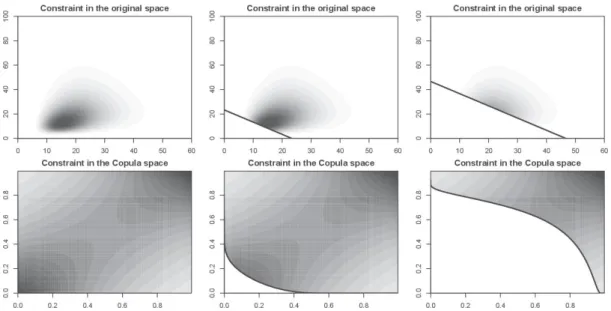
4.1 Frank copula with parameter 2, Log-Normal marginal c.d.f.’s, both with same µ= 3, andσ1 = 0.4,σ2 = 0.6. (Top row) Constraint in the original space, forB = 0,23,46

(Bottom row) Constraint in the Copula space, [0,1]2, for equivalent levels. . . 70

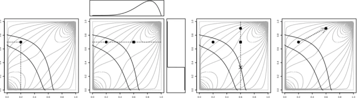
4.2 Example of the Global Beta kernel for a Gumbel(1.5) copula with Log-Normal marginals: (µ1 = 0.6, σ1 = 1.4), (µ2 = 0.4, σ2 = 1). The boundaries are such that F1−1(u1) +

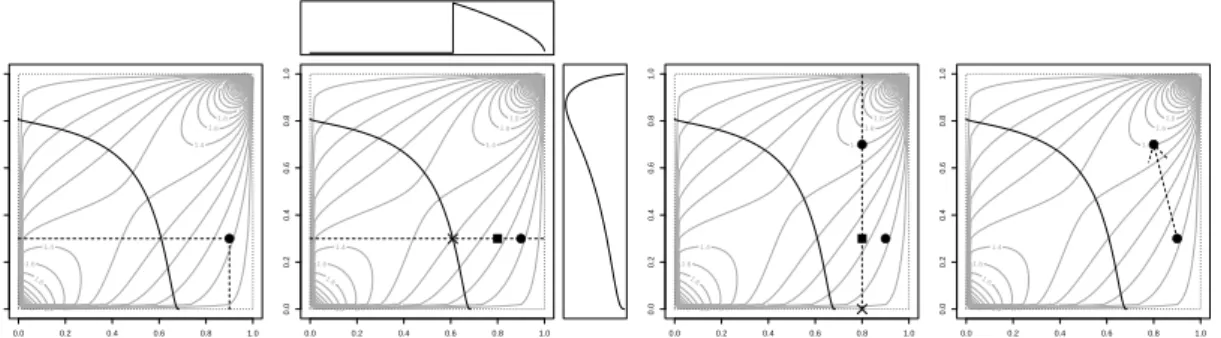
F₂−1(u2)>2.25 and 3.57. . . 73 4.3 Example of the move kernel for a Gumbel(1.5) copula with Log-Normal marginals: (µ1=

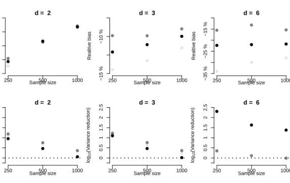
0.6, σ1 = 1.4), (µ2= 0.4, σ2= 1). The boundary is such thatF1−1(u1) +F2−1(u2)>3.57. 74 4.4 Coefficient of multivariate lower tail dependence for a 5-dimensional Clayton copula. 76 4.5 Relative Bias (top) and Variance Reduction (bottom) for the 5-dimensional

Clay-ton copula using the SMC algorithm. Using the notation from (4.8),•Marginal

fori= 1,•Marginal fori= 5,•Sum of all the marginal conditional expectations

(Expected Shortfall). . . 78 4.6 Ratio between the percentage of particles with non-zero weight and 1−α(top)

and Variance Reduction (bottom) for the 5-dimensional Clayton copula using the IS–ACH algorithm. Using the notation from (4.8), • Marginal for i = 1, • Marginal fori= 5,•Sum of all the marginal conditional expectations (Expected

Shortfall). . . 79 4.7 Coefficient of multivariate upper tail dependence for a Gumbel(1.25) copula. . . . 80 4.8 Relative Bias (top) and Variance Reduction (bottom) for the Gumbel(1.25) copula

using the SMC algorithm withNSM C= 250, 500 and 1,000 particles. Using the notation from (4.8),α= 0.999,•Marginal fori= 1,•Marginal fori=d,•Sum

(9)

List of Figures 9

4.9 Relative Bias (top) and Variance Reduction (bottom) for the Gumbel(1.25) copula using the SMC algorithm. Using the notation from (4.8),• Marginal fori= 1,• Marginal fori=d,•Sum of all the marginal conditional expectations (Expected

Shortfall). . . 82 4.10 Hierarchical Clayton Copula. . . 83 4.11 Relative Bias (top) and Variance Reduction (bottom) for the Hierarchical Clayton

copula from Figure 4.10 using the SMC algorithm with NSM C = 250 particles. Using the notation from (4.8),• Marginal fori= 1, •Marginal for i= 7,• Sum

of all the marginal conditional expectations (Expected Shortfall). . . 84 5.1 Quantile-Quantile plots, using the data from Figure 6.1, for the different LoBs

comparing (vertical axis) the empirical distribution of ZP Y |σ,D(t) based on Model Assumptions 5.3.1 and (horizontal axis) the log-normal approximation from Model Assumptions 5.3.11. . . 101 5.2 Quantile-Quantile plots, using the data from Figure 6.1, for the different LoBs

comparing (vertical axis) the empirical distribution ofZP Y | D(t) based on Model Assumptions 5.3.1 and (horizontal axis) the log-normal approximation from Model Assumptions 5.3.12 and using posterior samples as in Figures 6.5 and 6.6. . . 102 6.1 Cumulative claims payment (in millions of CHF). Lighter colours represent more

recent accident years. . . 122 6.2 Posterior distributions forσj for the MTPL line of business. One sees solid lines

representing the unnormalized posteriors, the histogram of the MCMC outputs and a red dashed line indicating the CL variance estimate. . . 124 6.3 Posterior distributions forσj for the Motor Hull line of business. One sees solid

lines representing the unnormalized posteriors, the histogram of the MCMC out-puts and a red dashed line indicating the CL variance estimate. . . 125 6.4 Posterior distributions forσjfor the Property line of business. One sees solid lines

representing the unnormalized posteriors, the histogram of the MCMC outputs and a red dashed line indicating the CL variance estimate. . . 126 6.5 Histogram of the parameterσP Y for the conditional model. Red dashed line: σP Y.127 6.6 Histogram of the parameterµP Y for the conditional model. Red dashed line: µP Y.128 6.7 Histograms levels used in the SMC sampler algorithm with p0 = 0.5 in the

marginalized model. The red dashed bar represents the true value of theαquantile.135

6.8 Histograms levels used in the SMC sampler algorithm in the conditional model. The red dashed bar represents the true value of theαquantile. . . 136

6.9 Bias for the marginalized model. . . 136 6.10 Bias for the conditional model. . . 137

(10)

6.11 Comparison between the “true” allocations (calculated via a large Monte Carlo

procedure) and the SMC sampler solution for the marginalized model. . . 138

6.12 Comparison between the “true” allocations (calculated via a large Monte Carlo procedure) and the SMC sampler solution for the conditional model. . . 139

6.13 Variance reduction for the marginalized model. . . 140

6.14 Variance reduction for the conditional model. . . 141

6.15 Relative bias in the marginalized model as a function of the parameterp0. . . 142

6.16 Relative bias in the marginalized model as a function of the sample size in the SMC sampler,NSM C. . . 143

7.1 Schematic representation of a LDA model. The aggregated loss in each year is represented hatched. . . 146

7.2 Individual Loss Policy (ILP) with TCL level of 1.5. . . 148

7.3 Accumulated Loss Policy (ALP) with ALP level of 2.0. . . 149

7.4 Schematic representation of the value function iteration. . . 151

7.5 Comparison of the two objective functions using the Accumulated Loss Policy (ALP): (top) histograms of the total loss under the global objective function (dark grey), local objective function (light grey), no insurance case (solid line); (bottom) Multiple optimal stopping times under the two loss functions. . . 164

7.6 Histogram of losses under four different stopping rules for the ALP case with (λ, µ, λN) = (3,2,3) and ALP = 10. . . 165

7.7 Histogram of losses under four different stopping rules for the ILP case with (λ, µ, λ e N) = (3,1,4) . . . 166

7.8 (Left) Histogram of the loss processZ =PN n=1Xn for X ∼LN(µ= 1, σ= 0.8) andN∼P oi(λN = 2) and in red the Gamma approximation using the first four moments ofZ. (Right) The graph of the region where the density is positive for all values ofz. . . 171

(11)

List of Tables

1.1 Composition of the Group of Ten (G-10) in 1974: original members (since

incep-tion, in 1962) and Switzerland (joined in 1964). . . 15

1.2 Example of risk weighted assets calculation under Basel I (from [Cruz et al., 2015]). 16 1.3 General summary of the Basel Accords (from [Cruz et al., 2015]). . . 18

1.4 Basel II business lines (left) and event types (right) – see [BCBS, 2006], Annexes 8 and 9. . . 20

2.1 Commonly used Archimedean generators . . . 26

2.2 Dependence measures (Spearman’s ρ, Kendall’s τ, lower and upper tail depen-dence) for Gaussian, Gumbel and Clayton copulas. . . 34

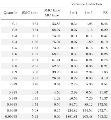
4.1 Computational time (in minutes) and Variance Reduction for the SMC algorithm when compared to a simple Monte Carlo scheme. . . 85

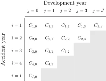
5.1 Claims triangle/trapezoid: The upper left triangle represents the information contained inD(t) and the lower right triangle (in gray) represents the unknowns, i.e.,Dc(_t). . . 88

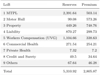
6.1 Original balance sheet. . . 115

6.2 SST’s (2015) standard development patterns for claims provision (normalized to have only 30 development years and then rounded to 2 digits). . . 116

6.3 Mack’s standard deviation estimates,sj, based on exogenous triangles. . . 117

6.4 Claims ratio, average claim amount (in millions of CHF) and market share. . . . 118

6.5 (Continued) Parameters and capital calculations for the marginalized and condi-tional models (Part II/II). . . 120

6.6 Copula correlation matrix from the marginalized model. . . 129

6.7 Correlation block for the marginalized model: ΩP Y . . . 129

6.8 Correlation block for the marginalized model: ΩP Y, CY,s . . . 129

6.9 Correlation block for the marginalized model: ΩCY,s . . . 129

6.10 Intermediate quantiles for different values ofp0. . . 130

7.1 Table of the value function for different L (steps remaining) and l stops in the Log-Normal example. . . 153

(12)

(13)

Chapter 1

Introduction to financial risk

management

The importance of financial risk management has been progressively increasing for all corpo-rations in the last few decades, notably in financial institutions. The first question one should pose is, then,what exactly is a financial risk? Although dictionaries would define risk as “the possibility of something bad happening” or “a situation involving exposure to danger”, in the context of financial risks the definition provided in [McNeil et al., 2010] is perhaps the most adequate one:

Financial risk is the quantifiable likelihood of loss or less-than-expected returns.

In a quantitative framework, the notion of risk is invariably related to uncertainty and, therefore, torandomness. The last concept has been formally defined in the first decades of the twentieth century with the axiomatization of the probability theory by A. N. Kolmogorov. As this thesis focuses on a quantitative approach to risk management we rely on the theories of probability and statistics.

Within the context of finance and insurance, three main risk classes can be characterized: market risk, credit risk and operational risk. The first risk, undoubtedly the one for which most of the attention has been drawn on the twentieth century, is related to “losses in positions arising from movements in market prices”, [BCBS, 2003b]. Credit risk, in turn, is the risk of not receiving agreed payments due to a default of the borrower or, more formally “the risk that a counterparty will not settle an obligation at its agreed full value, either when due or at any time thereafter”, [BCBS, 2003b]. Although market and credit losses are not desired, due to the nature of banking/insurance business, they can be seen asexpected. On the other hand operational losses, are comprised of a combination of both expected and unexpected losses and and comprise all the losses resulting from “inadequate or failed internal processes, people and systems, or from external events”, [BCBS, 2006]. From a quantitative point of view, another important notion that is universal in any quantification of risk management is that now known as model risk, which is associated with using an inappropriate model to measure risk. For example, one would be underestimating the risk of large losses if modelling the loss distribution

(14)

with lighter tails than the true (unobservable) distribution.

The definition of risk itself may already indicate why companies invest in measuring and understanding risk and loss processes but it is important to note that “earnings stability and the survival of the company are important managerial objectives”, [Hull, 2012]. Apart from the managerial objectives, risk management in financial institutions is also a regulatory requirement, as discussed in the next section.

1.1

Regulatory issues: Basel and Solvency accords

Unlike many other sectors of the economy, the financial sector, throughout the world, is heavily (and increasingly) regulated. Governments and their regulatory agencies want the sector to be as stable as possible, both locally (in their own countries) and globally, in an attempt to avoid repeated cycles of financial crisis and recessions/depressions of economies, which usually end up with expensive governmental bailouts (see [Reinhart and Rogoff, 2009] for a historical account on financial crisis). To ensure companies are going to be solvent in a finite horizon (of usually one year), regulators require them to set aside somecapital, which should be seen as a buffer to cover for unexpected losses.

As per [McNeil et al., 2015], “the main aim of modern prudential regulation has been to ensure that financial institutions have enough capital to withstand financial shocks and remain solvent. Robert Jenkins, a member of the Financial Policy Committee of the Bank of England, was quoted in theIndependenton 27 April 2012 as saying: Capital is there to absorb losses from risks we understand and risks we may not understand. Evidence suggests that neither risk-takers nor their regulators fully understand the risks that banks sometimes take. That’s why banks need an appropriate level of loss absorbing equity.”

In this section we provide an overview of how regulation in financial/insurance market has evolved since the 1970’s. The reader is referred to [BCBS, 2003a] for the history of the Basel Committee and to [Tarullo, 2008] for further details.

1.1.1

Banking regulation and the Basel Accords

The first modern attempt to design international regulatory standards in the banking industry dates back to 1974, when, in a cross-jurisdictional event, West Germany’s Federal Banking Supervisory Office forced the liquidation of the Bank Herstatt on the 26th of June. This event was followed by the bankruptcy of the Franklin National Bank of New York, in October and both are related to the breakdown (in the early 1970’s) of the Bretton Woods system of managed exchange rates.

As a response to these incidents, the Group of Ten (see Table 1.1) established, late in 1974, theCommittee on Banking Regulations and Supervisory Practices– to be later renamed to its current name, theBasel Committee on Banking Supervision(BCBS). Since 2009 the Committee is composed of 27 international bodies (see [BCBS, 2003a, Appendix A]).

(15)

1.1. Regulatory issues: Basel and Solvency accords 15

Belgium Netherlands Canada Sweden France Switzerland∗

Germany United Kingdom Italy United States Japan

Table 1.1: Composition of the Group of Ten (G-10) in 1974: original members (since inception, in 1962) and Switzerland (joined in 1964).

by improving supervisory knowhow and the quality of banking supervision worldwide. Even though the Committee does not possess any formal supranational authority, its supervisory standards are expected to be followed by the national supervisory authorities, with any necessary adjustments to the local jurisdiction. From a legal point of view, local authorities, e.g., Central Banks, are responsible for legally enforcing compliance with the guidelines set by the Committee.

1.1.1.1

Basel I: the Basel Capital Accord

Differently from the 1974 events whose origins trace back to Europeanmarket risk events, in the 1980’s the world would see acredit risk crisis in Latin America. The “lost decade” of 1980 in Latin America was preceded by boom years in the 1960’s and 1970’s, when local military dictatorships increased sovereign debts.

The Latin American debt crisis led the BCBS to develop the Basel Accord of 1988 (Basel I), whose main emphasis was on credit risk. This accord took an important step towards an international minimum capital standard, where thecapital requirement is to be understood as the amount of capital a financial institution is required to hold by it local regulator.

The 1988 Accord introduced a notion of simplerisk weights, where different classes of assets have different risk weights, ranging from 0% (for low risk assets) to 100% (for high risk assets). It is important to stress that the weights are defined by the local regulator but government bonds as well as cash, for example, usually have 0% weight while mortgages have 50% weight. Other types of loans to customers, in general, are assumed to have 100% weight. The sum of all assets weighted by its risk weight leads to the so-called Risk Weighted Assets (RWA). An example of the risk-weighting process (from [Cruz et al., 2015]) can be seen in Table 1.2

Another concept introduced in the first Basel accord was the classification of the capital into Tier 1 and Tier 2, as described in [BCBS, 1988, Annex 1]:

• Tier 1 (core capital)

(a) Paid-up share capital/common stock; (b) Disclosed reserves.

(16)

Risk weight (%) Asset Amount ($) RWA ($)

0 Cash 10 0

Treasury bills 50 0

Long-term treasury securities 100 0

20 Municipal bonds 20 4

Items in collection 20 4

50 Residential mortgages 300 150

100 AA+ rated loan 20 20

Commercial loans, AAA- rated 55 55

Commercial loans, BB- rated 200 200

Sovereign loans B- rated 200 200

Fixed assets 50 50

Not rated Reserve for loan losses (10) (10)

Total 1015 673

Table 1.2: Example of risk weighted assets calculation under Basel I (from [Cruz et al., 2015]). (a) Undisclosed reserves;

(b) Asset revaluation reserves;

(c) General provisions/general loan-loss reserves; (d) Hybrid (debt/equity) capital instruments; (e) Subordinated debt.

The main requirement of the Basel I accord (implemented by the end of 1992) was that the Capital Adequacy Ratio (CAR) should be at least 8%, where the CAR (also known as Cooke ratio) is defined as the percentage of the institution’s eligible capital (sum of Tier 1 and Tier 2 capital) to its RWA. In other words,

CAR =Eligible capital

RWA ≥8%. (1.1)

Remark 1.1.1. As mentioned in Paul Embrecht’s presentation [Embrechts, 2008] the

calcula-tion of the capital ratio in (1.1) can be divided between “us” and “them”. The denominator, which involves the risk weighted positions, is calculated by “us”, the ‘quants’, while “they”, the accountants, the management and the board are responsible by the numerator.

1.1.1.2

Basel II: the New Capital Framework

One of the significant weaknesses of the 1988 Accord was that thecredit rating of the borrower was not taken into consideration when calculating the risk weight of its debt.

To correct for this discrepancy and to include other features, in 1999, a decade after the release of the first Basel Accord the BCBS started the process to replace the 1988 Accord. The

(17)

result was theRevised Capital Frameworkor theBasel II, released in June 2004. This document comprised threepillars, namely,

1. Pillar 1 - Minimum capital requirements; 2. Pillar 2 - Supervisory review;

3. Pillar 3 - Market discipline.

In the first Pillar, the total capital did not change and banks were still required to hold at least 8% of the RWA, but the credit worthiness of the counterparts started to be reflected. While the original Basel I Accord only dealt withcredit risk(with the 1996 Amendment including market risk) the Basel II Accord created a capital charge also foroperational risk.

As noticed by [Hull, 2012], due to Pillar 2 “supervisors were required to do far more than just ensuring that the minimum capital required under Basel II is held”. Some of the new attribution of the local regulators were, for example, to encourage banks to develop new risk management techniques and also to help financial institutions to evaluate risks not covered in Pillar 1.

The third Pillar required banks to publicly disclose the risk measures and any other infor-mation relevant to risk management, including how they allocate their capital. The allocation of capital is one of the main themes of this thesis, being discussed in Chapters 4 and 6. It has also been decided that the capital should be calculate as the Value at Risk (VaR) with a one-year time horizon and a 99.9% confidence level for operational risk.

To overcome banks’ criticism about the coarseness of the risk weights from Basel I, in the new Accord banks were allowed to choose from three different approaches for handling credit risk:

1. The Standardized Approach;

2. The Foundation Internal Ratings Based (IRB) Approach; 3. The Advanced IRB Approach.

Even the most basic alternative (the Standardized Approach) already included some measures for better differentiation of risks throughcredit ratings, although the ratings themselves are not calculated internally when the bank chooses this approach. Larger and more complex banks were allowed to use Internal Ratings Based (IRB) approaches. In these cases the assessment of the riskiness of the credit portfolio could be done by the bank itself.

As mentioned in [McNeil et al., 2015], “a basic premise of Basel II was that the overall size of regulatory capital through the industry should stay unchanged under the new rules. Since the new rules for credit risk were likely to reduce the credit risk charge, this opened the door for operational risk”. For the operational risk capital three approaches were introduced:

(18)

Accord Year Key points

Basel I 1988 Introduces minimal capital requirements for the banking book. Introduces tier concept for capital requirement.

Incorporates trading book into the framework later on through the Market Risk Amendment (MRA).

Basel II 2004 Allows usage of internal models and inputs in risk management. Introduces operational risk.

Basel II/III 2010 Increases capital requirement for trading book, with significant increase for correlation trading and securitization.

Basel III 2010 Motivated by the financial crisis of 2008, increases capital

requirements, introduces leverage constraints and minimum liquidity and funding requirements.

Table 1.3: General summary of the Basel Accords (from [Cruz et al., 2015]).

2. The Standard Approach (SA);

3. The Advanced Measurement Approach (AMA).

As with the credit risk, the use of these approaches depend on the level of sophistication of the bank. Under the BIA the operational risk capital is set as the bank’s average annual gross income over the last three years multiplied by 0.15. Under the SA approach there are different factors to be applied to the gross income from different business lines, this been the only difference from the BIA. In the AMA the bank is allowed to use its own internal models to calculate the operational risk capital. Another advantage of this approach is that the regulator can recognize the risk mitigation impact of insurance contracts (see Chapter 7).

1.1.1.3

Basel III

After an European trigger (1974) and a Latin American one (1980’s) the 2000’s witnessed an American born crisis (named by some as “The Crisis” [Das et al., 2013]), which, as usual, led to more regulation: this time the Basel III Accord. A summary of the key tekaways (compiled in [Cruz et al., 2015]) of the Basel Accords is found in Table 1.3.

The first proposals of the Basel III document were published in December 2009 but the final version was only available a year later, see [BCBS, 2010b] and [BCBS, 2010a] and its implementation will occur gradually between 2013 and 2019. As discussed in [Hull, 2012], there are six parts to this regulatory document:

1. Capital Definition and Requirements; 2. Capital Conservation Buffer;

(19)

4. Leverage Ratio; 5. Liquidity Risk;

6. Counterparty Credit Risk.

At the moment these lines are being written the supervisors at the BCBS are consulting the operational risk community on the possibility of scrapping the Advanced Measurement Approach (AMA), in a movement that started in October 2014. By that time the BCBS released the consultation document [BCBS, 2014] proposing a Revised Standardized Approach (RSA) for operational risk and in March 2016 the BCBS published the consultative document [BCBS, 2016b] which suggests the replacement of the AMA by a new non-model-based method, named Standardized Measurement Approach (SMA). The SMA is based on the combination of a simple standardized measure of operational risk, based on a fixed percentage of operating revenues, and bank-specific operational loss data (based on the arithmetic average of losses over the past 10 years). As this proposal discards the knowledge on operation risk modelling accumulated both by practitioners and academics it has been followed by a heated debate (see, e.g., [Peters et al., 2016a] and [Wills, 2016]).

1.1.2

Insurance regulation: Solvency I/II and the Swiss Solvency Test

Notwithstanding that banks have supranational regulatory standards, insurance companies, up to date, do not have any formal international regulation. In the United States insurance com-panies are regulated at the state level, with the national support of the National Association of Insurance Commissioners (NAIC). In Europe the European Union is in charge of the reg-ulatory role, through the European Insurance and Occupational Pensions Authority (EIOPA, formerly known as CEIOPS: the Committee of European Insurance and Occupational Pensions Supervisors). On the other hand, since the 1st of January 2011, Switzerland has been using the Swiss Solvency Test (SST) for capital calculation, over-sighted by the Swiss Financial Markets Supervisory Authority (FINMA), a government body created in 2007 as a merge of the Fed-eral Office of Private Insurance (FOPI), the Swiss FedFed-eral Banking Commission (EBK) and the Anti-Money Laundering Control Authority.

The recently replaced European regulatory framework, known as Solvency I, came to force in 2004 and was replaced by Solvency II (often called “Basel for insurers”) on the 1st of January 2016. While Solvency I calculated capital only for underwriting risks, the new directive has a much wider scope, considering, for example, operational risk capital. The informal name of the Solvency II directive is mainly due to the similarities it holds with Basel II. For example, under Solvency II there are also be three pillars, exactly as in Basel II.

Pillar 1 of Solvency II introduces two capital requirements, the Solvency Capital Require-ment (SCR, discussed in Section 5.2.3) and the Minimum Capital RequireRequire-ment (MCR). The SCR can be calculated using either a standard formula given by the regulators or an internal model developed by the insurance company. This is the capital required to ensure the company

(20)

Business line

1 Corporate finance

2 Trading and sales

3 Retail banking

4 Commercial banking

5 Payment and settlement

6 Agency services 7 Asset management 8 Retail brokerage Event type 1 Internal fraud 2 External fraud

3 Employment practices and workplace safety

4 Clients, products and business practices

5 Damage to physical assets

6 Business disruption and system failures

7 Execution, delivery and process management

Table 1.4: Basel II business lines (left) and event types (right) – see [BCBS, 2006], Annexes 8 and 9.

will be able to meet its obligations over the next 12 months and if the capital falls bellow the SCR level the company should, at least, deliver a plan to the supervisor to restore its capital. Differently from Basel II, in the Solvency II regulation the capital involves the calculation of a Value at Risk (VaR) with 99.5% confidence (less than Basel II’s 99.9% for OpRisk, for example),

while the SST prescribes the calculation of the 99% Expected Shortfall (ES).

The MCR, which is intended to correspond to the VaR85%(and is bounded between 25%

and 45% of the SCR), can be regarded as a “hard” capital floor (while the SCR is a “soft” floor), a control level that, if breached, would trigger “ultimate supervisory action”. In this case the “the insurer’s liabilities will be transferred to another insurer and the license of the insurer will be withdrawn or the insurer will be closed to new business and its in-force business will be liquidated” (as stated in the European Commission MEMO/07/286).

1.2

Research questions and outline of the thesis

This thesis studies two different problems related to financial companies’ capital. The first one is related tounderstandingthe capital, in a process calledallocation. In this regard we develop Sequential Monte Carlo (SMC) algorithms to compute the capital and also to break it down into the company’s different constituents. The second problem is related to the capitalmanagement, where we develop insurance products to facilitate the transference of specific risks.

These problems are studied in two different contexts. The capital allocation problem is first presented as a way to understand the drivers of the capital related to operational risk, for example, distributing the capital amongst the combination of business lines and event types, as in Table 1.4. An idealized version of this problem is discussed in Chapter 4, when we first introduce a Sequential Monte Carlo algorithm to calculate, via simulation, the capital contributions. In this first instance we assume all the model parameters are perfectly known and focus solely on the allocation problem, which can be rewritten as an expectation conditional to a rare event. These results were published in [Targino et al., 2015].

Chapters 5 and 6 deal with the same allocation problem, in an actuarial context. Moti-vated by the short term view of the recent solvency regulations (such as the Swiss Solvency

(21)

1.2. Research questions and outline of the thesis 21

Test and Solvency II), Chapter 5 is devoted to developing statistical models for theone-year reserve risk and theone-year premium risk. The later is constructed based on the Swiss Sol-vency Test directives and no parameter uncertainty is involved. For the former we extend the Bayesian gamma-gamma chain ladder model of [Gisler, 2006] and [Gisler and W¨uthrich, 2008] and provide two distinct approximations to it, resulting in what we call the marginalized and conditional models. Both strategies approximate the Bayesian gamma-gamma model through log-normal distributions and matching of the first two moments, the difference being at which stage the approximation is performed. For the marginalized version we match the moments of a distribution where the unknown parameters have been integrated out, while in the conditional model we approximate the conditional distribution of the Bayesian gamma-gamma model by a log-normal.

In Chapter 6 we make use of the framework developed in Chapter 5 and present algorithms to solve the allocation problem under the marginalized and conditional approximations. As in the marginalized approach no parameter uncertainty is present (it is integrated out before the allocation process) the algorithm is mostly based on the one provided in Chapter 4. Allocations for the conditional model present an additional layer of complexity, as one needs to calculate conditional expectations with respect to a model whose density is not known in closed form. To overcome this difficulty we develop apseudo-marginal SMC sampler.

Technical findings related to the extension of the Bayesian gamma-gamma chain ladder model are presented in [Peters et al., 2017] and its use in the capital allocation problem is detailed in [Peters et al., 2016b].

Chapter 7 returns the focus to operational risk modelling, and the aim is not to understand the capital anymore, but to construct instruments for the transference of risk, which would lead to capital reductions. In particular, we study a class of insurance products where the policy holder (say, a bank) has the option to insurekof its annual operational risk losses in a horizon

of T years. This involves a choice of k out of T years in which to apply the insurance policy

coverage by making claims against losses in the given year. Although this class of products can be used for mitigation of any risk, is particularly relevant for operational risk, due to the sheer scale of operational losses – which leads to expensive insurance products. As the buyer is only covered fork years (and notT) this type of product can substantially reduce insurance

premiums, making it affordable to a larger proportion of companies.

The insurance product structure presented in Chapter 7 can accommodate any kind of annual mitigation, but we present two basic generic insurance policy structures that can be combined to create more complex types of coverage. Following the Loss Distributional Approach (LDA) with Poisson distributed annual loss frequencies and Inverse-Gaussian loss severities we are able to derive analytical expressions for the multiple optimal decision strategy that minimizes the expected operational risk loss over the nextT years. For the cases where the combination

(22)

optimal decision rules, we also develop a principled class of closed form approximations to the optimal decision rule. These approximations are developed based on a class of orthogonal Askey polynomial series basis expansion representations of the annual loss compound process distribution and functions of this annual loss. The results from this chapter are published in [Targino et al., 2016].

1.3

List of publications and pre-prints

Publications

1. G.W. Peters; R.S. Targino; P. Shevchenko Understanding Operational Risk Capi-tal Approximations: First and Second Orders (2013) Governance and Regulation, 2(3)

(arXiv:1303.2910). (Invited Special Issue to coincide with 8th International conference “International Competition in Banking: Theory and Practice”, Sumy, Ukraine, 2013.)

2. R.S. Targino; G.W. Peters; P. Shevchenko Sequential Monte Carlo Samplers for

capi-tal allocation under copula-dependent risk models (2015). Insurance: Mathematics and

Economics, 61 (doi:10.1016/j.insmatheco.2015.01.007).

3. R.S. Targino; G.W. Peters; G. Sofronov; P. ShevchenkoOptimal exercise strategies for

operational risk insurance via multiple optimal stopping times (2016). Methodology and

Computing in Applied Probability (doi:10.1007/s11009-016-9493-8).

Pre-prints

1. G.W. Peters;R.S. Targino; M.V. W¨uthrichFull Bayesian Analysis of Claims Reserving Uncertainty (2016) Available at SSRN 2783223, version of 20/May/2016.

2. G.W. Peters;R.S. Targino; M.V. W¨uthrichBayesian modelling and allocation of insur-ance risks. (2016) Manuscript in preparation.

3. C. Chimisov; R.S. Targino; G.W. Peters Risk allocation and risk parity portfolios in high dimensions using Gibbs samplers (2016) Manuscript in preparation.

(23)

Chapter 2

Copulas and risk allocation

This chapter present some background material in the theory of copulas and the mathematical formulation of the capital allocation problem. In particular, we describe the classes of copulas that are used throughout the thesis, as well as some of their properties, with special focus on measures of dependence. In this regard, Section 2.1.3.1 provides a complete picture of the bounds on correlations under a multivariate model described by a Gaussian copula and log-normal marginals. The formulation of the capital allocation problem is provided in Section 2.2. In this section we also discuss how to “coherently” perform the allocation process in a hierarchical structure.

2.1

Copulas and Sklar’s theorem

Although the concept of “copula” can be traced back to the seminal work of Abe Sklar [Sklar, 1959], where the mathematical term was introduced, (see [Sklar, 1996]) or even the earlier works of Wassily Hoeffding and Maurice Fr´echet, its importance in Finance / Ac-tuarial Science was only realized in the late 1980’s / early 1990’s. The reader is referred to [Dall’Aglio et al., 1991] for a discussion on the early contributions to the field of copulas; [Frees and Valdez, 1998] and [Embrechts et al., 2002] for some of the publications that boosted the actuarial and financial applications; and [Joe, 1997], [Cherubini et al., 2004], [Nelsen, 2007] and [Joe, 2014] for book-length introductions to the topic.

As with any scientific field, though, copulas were not a unanimity amongst all the re-searchers and the field saw some interesting academic debate in the past decade, including the one sparked by [Mikosch, 2006] and followed up by academic responses and a rejoinder in the same journal. Unfortunately we also witnessed some shallow non-academic discussion after the 2006+ financial crisis, led by the (in)famous 2009’s Wired magazine article [Salmon, 2009] where the author blames the Gaussian copula (see Section 2.1.2 below) model of [Li, 2000] for the financial meltdown in 2006+. Some academic responses to this discussion can be found in [Donnelly and Embrechts, 2010] and, more recently, in Paul Embrechts’ interview published as [Durante et al., 2015], while a non-technical defense was provided in The EconomistâĂŹs article [Anonymous, 2009].

(24)

At this point we pose the same question asked and promptly answered in [Nelsen, 2007]: What are copulas? From one point a view, copulas are functions that join or “couple” multi-variate distribution functions to their one dimensional marginal distribution functions. Alter-natively, copulas are multivariate distribution functions whose one-dimensional marginals are uniform on the interval (0,1). The latter definition is formalized below.

Definition 2.1.1 (Copula). A d-dimensional copula is a distribution function on [0,1]d _with

uniform marginal distributions.

From a modelling point of view, the importance of copulas is summarized by the following elegant and fundamental theorem, which shows that a copula can be extracted from every multivariate distribution function and also that the combination of a copula and univariate distributions leads to a well defined multivariate distribution. For a proof see, for example, [McNeil et al., 2010, Theorem 5.3].

Theorem 2.1.2(Sklar). Let FX be a joint distributions with marginalsF1, . . . , Fd and denote

R=R∪ {−∞,+∞}. Then there exists a copula C: [0,1]d_→[0_,1]_{such that}

FX(x) =C F1(x1), . . . , Fd(xd)

, ∀x= (x1, . . . , xd)∈Rd. (2.1)

If the marginals are continuous then C is unique, and given by

C(u1, . . . , ud) =FX(F₁−1(u1), . . . , Fd−1(ud)).

Conversely, if C is a copula and F1, . . . , Fd are univariate distributions, then the distribution

FX defined in (2.1) is a joint distribution function with marginalsF1, . . . , Fd.

Moreover, if we assume thatF1, . . . , Fd are differentiable, then the joint density function of

Xcan be written as fX(x) =c F1(x1), . . . , Fd(xd) d Y i=1 fi(xi), where c(u1, . . . , ud) = ∂ d_C(_u 1, . . . , ud) ∂u1. . . ∂ud andfi is the density of Xi.

Another important result in the theory of copulas is the so-called Fr´echet-Hoeffding bounds Theorem, stated below.

Theorem 2.1.3 (Fr´echet-Hoeffding bounds Theorem). For any d-dimensional copula C the

following bounds hold: max ( d X i=1 ui+ 1−1,0 ) ≤C(u)≤min{u1, . . . , ud}.

The lower and upper Fr´echet-Hoeffding bounds are usually denoted, respectivelyW(u) and

M(u).

In the sequel we branch into two distinct ways of creating copula functions. First, we explicitly define the functional form of the copula and later we extract the copula of known multivariate random variables, generating, respectively, explicit and implicit copulas.

(25)

2.1. Copulas and Sklar’s theorem 25

2.1.1

Explicit copulas and Archimedean copulas

Before discussing the class ofArchimedeancopulas we first introduce threefundamental copulas: the independence, comonotonicity and countermonotonicity.

Definition 2.1.4. The d-dimensional independence and comonotonicity copulas are defined,

respectively, as

Π(u) = d Y

i=1

ui, and M(u) = min{u1, . . . , ud}. The countermonotonicity copula is the two-dimensional copula defined as

W(u) = max{u1+u2−1,0}.

It can be seen from Sklar’s Theorem that continuous random variables are independent if, and only if, its copula is the independence copula from Definition 2.1.4.

The comonotonicity copula from Definition 2.1.4 is precisely the Fréchet-Hoeffding upper bound, while the countermonotonicity copula is the two-dimensional Fréchet-Hoeffding lower bound (see [McNeil et al., 2010, Example 5.21] for a proof that ford >2 the Fréchet-Hoeffding

lower bound is not a copula).

Based on the comonotonic and countermonotonic copulas we now define two important concepts of dependence: comonotonicity and countermonotonicity.

Definition 2.1.5(Comonotonicity / Countermonotonicity). The random variablesX1, . . . , Xd

are said to be comonotonic if they admit the Fr´echet-Hoeffding upper bound as copula.

The random variablesX1andX2are said to be countermonotonic if they admit the Fr´ echet-Hoeffding lower bound as copula.

The following two properties give some insight on the precise meaning of the comonotonicity / countermonotonicity concepts. The proofs can be found in [McNeil et al., 2010, Proposition 5.6 and Proposition 5.19].

Proposition 2.1.6. The random variables(X1, . . . , Xd)are comonotonic if, and only if,

(X1, . . . , Xd)= (d v1(Z), . . . , vd(Z)),

for some random variableZ and increasing functionsv1, . . . , vd.

The random variablesX1 andX2 are countermonotonic if, and only if, (X1, X2)= (d t1(Z), t2(Z)),

for some random variableZ witht1 increasing andt2 decreasing or vice-versa.

In order to introduce a class of copulas called Archimedean copulas we first define the concept of the generator of a copula, which is a function of a parameter θ. Some commonly

(26)

Definition 2.1.7 (Archimedean generator). An Archimedean generator is a continuous, de-creasing function ψθ: [0,∞]→[0,1]that satisfies ψθ(0) = 1, limt→∞ψθ(t) = 0and is strictly

decreasing on [0, inf{t : ψθ(t) = 0}].

Definition 2.1.8 (Archimedean copulas). A d-dimensional copula is called Archimedean if it

is of the form

C(u; ψθ) =ψθ(ψ_θ−1(u1) +. . .+ψθ−1(ud)), u= (u1, . . . , ud)∈[0,1]

d_, _(2.2) whereψθ is the Archimedean generator.

Remark 2.1.9. The name Archimedean in the context of copulas come, as discussed in

[Nelsen, 2007, Section 4.3], from the Archimedean “axiom” from abstract algebra. The “ax-iom” is indeed a property held by some algebraic structures, but the name was coined by the Austrian mathematician Otto Stolz, as it appears in Archimedes’ “On the sphere and cylinder” work as Axiom V.

Family Parameter Generatorψθ(t)

Clayton θ∈(0,∞) (1 +t)−1/θ

Gumbel θ∈[1,∞) exp{−t1/θ_}

Table 2.1: Commonly used Archimedean generators

Although Archimedean copulas may be sufficiently flexible for low (2 to 5) dimensions, it becomes very restrictive as the dimensionality increases, as there is typically a single parameter driving all the dependence structure. Another drawback of Archimedean copulas is the fact that the dependency is symmetric with respect to permutation of variables.

Several alternative classes of copulas have been proposed in the literature lately, in-cluding pair copulas (see [Aas et al., 2009]), factor copulas (see [Oh and Patton, 2013] and [Krupskii and Joe, 2013]) and Hierarchical Archimedean Copulas (HAC), also known as nested Archimedean copulas (see, for example, [Embrechts et al., 2003, Section 6.5] and [Hofert, 2010]). We briefly describe the latter in the sequel, based on [Okhrin and Ristig, 2014].

HAC considers the composition of simple Archimedean copulas (as the ones described in Table 2.1) as follows. A d-dimensional HAC is denoted by C(u1, . . . , ud; s,θ), where θ

denotes the vector of feasible dependency parameters (see discussion below). The parameter

s= (. . .(igik)il. . .) denotes the structure of the entire HAC, whereim∈ {1, . . . , d : g6=k6=l} is a reordering of the indexes of the variables with m = 1, . . . , d and g, k, l ∈ {1, . . . , d : g 6= k 6=l}. Structures of subcolulas are denoted by sj with s = sd−1. An example, taken from

[Okhrin and Ristig, 2014] is presented in Figure 2.1.

Generators for HAC may come from different families of Archimedean copulas, but care should be taken, as the resulting structure may not be a copula (see [McNeil, 2008, Theorem 4.4]). For generators within the same family, a sufficient condition for the HAC to be a proper

(27)

2.1. Copulas and Sklar’s theoremJournal of Statistical Software 3 27 ● u1 u2 u3 u4 θ((u1.u2).u3)=3 θ(u1.u2)=4 θ(((u1.u2).u3).u4)=2 ● u4 u3 u1 u2 θ(u4.u3)=3 θ(u1.u2)=4 θ((u4.u3).(u1.u2))=2

Figure 1: Fully and partially nested Archimedean copulae of dimensiond= 4 with structures

s= (((12)3)4) on the left ands= ((43)(12)) on the right.

copulae. The functionφ(·) is called the generator of the copula and commonly depends on a single parameterθ. For example, the Gumbel generator is given byφθ(x) = exp(−x1/θ) for

0≤x <∞, 1≤θ <∞. Detailed reviews of the properties of Archimedean copulae can be found inMcNeil and Neˇslehov´a(2009) and inJoe(1997).

A disadvantage of Archimedean copulae is the fact that the multivariate dependency structure is very restricted, since it typically depends on a single parameter of the generator function

φ(·). Moreover, the rendered dependency is symmetric with respect to the permutation of variables, i.e., the distribution is exchangeable. HAC (also called nested Archimedean copulae) overcome this problem by considering the compositions of simple Archimedean copulae. For example, the special case of four-dimensional fully nested HAC can be given by

C(u1, u2, u3, u4) =C3{C2(u1, u2, u3), u4} (2)

=φ3{φ−₃1◦C2(u1, u2, u3) +φ−31(u4)},

whereCj(u1, . . . , uj+1) =φj[φ−j1{Cj−1(u1, . . . , uj)}+φ−j1(uj+1)],j= 2, . . . , d−1, andC1=

φ1{φ−11(u1) +φ1−1(u2)}. The functional form ofCj(·) indicates that the composition can be

applied recursively. A different segmentation of the variables leads naturally to more complex HAC. In the following, let d-dimensional HAC be denoted by C(u1, . . . , ud;s, θθθ), where θθθ

denotes the vector of feasible dependency parameters ands= (. . .(igik)i`. . .) the structure

of the entire HAC, whereim∈ {1, . . . , d}is a reordering of the indices of the variables with m = 1. . . , d, and g, k, ` ∈ {1, . . . , d :g 6= k 6= `}. Structures of subcopulae are denoted bysj withs=sd−1. For instance, the structure according to Equation2iss= (s2)4 with

sj= (sj−1(j+1)),j= 2,3, for the sucopulae ands1= (12). A clear definition of the structure

is essential, assis in fact a parameter to estimate. Thus, Equation2can be rewritten as

C(u1, u2, u3, u4;s= (((12)3)4), θθθ) =C{u1, u2, u3, u4; (s24),(θ1, θ2, θ3)>} = φθ3(φ− 1 θ3 ◦C2{u1, u2, u3; (s1(3)),(θ1, θ2) >_}₊_φ−1 θ3(u4)).

Figure1presents the four-dimensional fully and partially nested Archimedean copula. HAC can adopt arbitrarily complex structuress. This makes it a very flexible and simul-taneously parsimonious distribution model. The generators φθj(·) within a single nested

Figure 2.1: Fully (left) and partially (right) nested Archimedean copulas of dimensiond= 4 with s= (((12)3)4) ands= ((43)(12)), respectively. Figure taken from [Okhrin and Ristig, 2014].

copula is to have decreasing parameters from the highest to the lowest level (see, for example, [Hofert, 2010]).

2.1.2

Implicit copulas and the Gaussian copula

In order to characterize the well known Gaussian copula we first discuss the meaning of implicit copulas, extracted from known multivariate distributions.

Definition 2.1.10. (Copula of F) If Y has joint distribution function FY with continuous

marginal distributionsFY1, . . . , FYd, then the copula ofF (also called the copula ofY) is defined

as the distribution function of FY1(Y1), . . . , FYd(Yd)

, i.e., CY(u) =P[FY1(Y1)≤u1, . . . , FYd(Yd)≤ud] =P[Y1≤FY−11(u1), . . . , Yd≤F −1 Yd(ud)] =FY FY−11(u1), . . . , F −1 Yd(ud) .

Given this definition of the implicit copula of F, we can now derive the density of this

copula, namely c(u1, . . . , ud) =∂ d_C(_u 1, . . . , ud) ∂u1. . . ∂ud = fY F −1 Y1 (u1), . . . , F −1 Yd(ud) fY1(F −1 Y1 (u1))× · · · ×fYd(F −1 Yd(ud)) .

The next proposition (see [McNeil et al., 2010, Proposition 5.6] for a proof) states an im-portant result related to transformations of marginals.

Proposition 2.1.11 (Invariance). Let (Y1, . . . , Yd) be a random vector with

continu-ous marginals and copula C and let T1, . . . , Td be strictly increasing functions. Then

T1(Y1), . . . , Td(Yd)also has copula C.

Using Sklar’s Theorem we can now define the so-called Gaussian copula, which is part of the class of implicit copulas (those extracted from known multivariate distributions).

(28)

Definition 2.1.12. (Gaussian copula) IfY∼N(µ,Σ)denotes a multivariate gaussian random variable with mean vector µ and covariance matrix Σ, then its copula is called the Gaussian copula.

Note that if we define P = ρ(Σ) as the correlation matrix of Y then Proposition 2.1.11

ensures that the copula for Y is the same as the copula of X ∼ N(0, P). Therefore, from

Definition 2.1.10 the Gaussian copula is given by

CGa Σ (u) =P[Φ(X1)≤u1, . . . ,Φ(Xd)≤ud] = Φ0,P Φ−1(u1), . . . ,Φ−1(ud), with density cGa Σ (u) = φ0,P Φ −1(_u 1), . . . ,Φ−1(_ud) φ(Φ−1(_u 1))× · · · ×φ(Φ−1(ud))

where Φµ,Σ(·) andφµ,Σ(·) denotes, respectively, a (multivariate) normal distribution and density functions with meanµand covariance matrix Σ. Without explicit mention toµand Σ, Φ(·) and φ(·) denote, respectively, the standard univariate normal distribution and density. If we define

q= (q1, . . . , qd) as the normal scores, i.e.,qi= Φ−1(ui) then the density of the Gaussian copula can be simplified to cGa Σ (u) = (2π) −d/2_|_P_|−1/2exp −1₂qTP−1_q Qd i=1(2π)−1/2exp −1₂q2i =|P|−1/2exp −1 2qT(P−1−I)q ,

where|P|=det(P). Note that the Gaussian copula is parametrized by thed(d−1)/2 parameters

of the correlation matrix.

In summary, if we want a multivariate random variableX= (X1, . . . , Xd) to have arbitrary

marginals FX1, . . . , FXd and the dependence structure to be given by a Gaussian copula with

correlation matrixP, then its distribution and density functions should be, respectively, FX(x) = Φ0,P Φ−1(FX1(x1)), . . . ,Φ −1₍_F Xd(xd)) ; fX(x) =|P|−1/2exp −1 2qT(P−1−I)q d Y i=1 fXi(xi),

where here the normal scores are defined asqi= Φ−1 FXi(xi)

.

Alternatively, let us now assume we have a r.v. X ∼ N(0,Σ), with (Σ)i,i = σ2i and (Σ)i,j = 0 ifi6=j. In other words,Xi∼N(0, σi2) and Xi is independent of Xj ∀j 6=i. Given this model forX, we want to find the correlation matrixP of the Gaussian copula that couples

the marginalsXi∼N(0, σi2) and return us a joint distributionX∼N(0,Σ).

First note that ifXi∼N(0, σi2) then its distribution and density functions can be written in terms of standard normal’s c.d.f. and p.d.f. as follows:

(29)

2.1. Copulas and Sklar’s theorem 29

Therefore the joint p.d.f. ofXcan be written as

fX(x) =cGa P F1(x1), . . . , Fd(xd) d Y i=1 fi(xi) =|P|−1/2_exp −1 2qT(P−1−I)q d Y i=1 φ(xi/σi)σi−1, whereqi= Φ−1 Fi(xi)= Φ−1 Φ(xi/σi)=xi/σi.

From the above formula, however, it is not clear what should be the choice forP in order

to haveX∼N(0,Σ). To overcome this difficulty, letWbe such thatWi= X_σ_ii, fori= 1, . . . , d. It then implies thatXi=σiWi and that

∂x ∂w = ∂x1 ∂w1 . . . ∂x1 ∂wd ... ... ... ∂xd ∂w1 . . . ∂xd ∂wd = σ1 . . . 0 ... ... ... 0 . . . σd = d Y i=1 σi

Therefore, the p.d.f. of the transformed random variable is given by

fW(w) =fX(σ1w1, . . . , σdwd) d Y i=1 σi =|P|−1/2_exp −1 2wTP−1w exp−1 2wTw d Y i=1 φ(wi) = (2π)−d/2_|_P_|−1/2exp −1 2wTP−1w .

From this relationship we can deduce thatW∼N(0, P) thus we can see thatX∼N(0,Σ)

with

Σi,i=V ar(σiWi) =σ2iV ar(Wi), Σi,j=Cov(Xi, Xj) =σiσjCov(Wi, Wj).

Since the variance-covariance matrix of W, namely P, is a correlation matrix we have that Pi,i= 1 and Pi,j= Σi,j/(σiσj).

2.1.3

Dependence measures

As we saw in Sklar’s Theorem, the copula function encompasses the whole dependence structure of a multivariate random variable. Therefore, it is natural to develop scalar dependence measures that explain, in some sense, the strength of the dependence. In the sequel we discuss three different types of dependence measures: (1) linear correlation; (2) rank correlation; and (3) coefficients of tail dependence (and its extension to the multivariate case).

2.1.3.1

Linear correlation

Linear correlation is certainly one of the most well known concepts in Statistics and some misconceptions around it are discussed in length in [Embrechts et al., 2002]. In this section we focus on one particular point, related to the attainability of prescribed correlations on a specific model, as it is an important regulatory requirement (as discussed in Chapter 6).

(30)

As discussed, for example in [Embrechts et al., 2002, Fallacy 2], for given marginal distri-butions not all linear correlations between -1 and 1 can be achieved. This can also be seen in the following Lemma (see [Denuit and Dhaene, 2003, Section 2]).

Lemma 2.1.13 (Correlation bounds). Let (X1, X2) be a bivariate random variable with

marginal distributionsF1 andF2. Then the correlation between X1 andX2 is bounded by Cov(F₁−1(U), F₂−1(1−U)) pVar( X1)Var(X2) ≤ Corr(X1, X2)≤ Cov(F −1 1 (U), F2−1(U)) pVar( X1)Var(X2)

forU uniformly distributed in [0,1].

Although theoretically interesting, Lemma 2.1.13 may provide bounds that are too wide and in some cases just state that the correlation lies between−1 and 1. In the sequel we show that

in the particular case of a random vector with Log-Normal marginals and dependence structure Gaussian copula it is possible to calculate precisely the intended correlation and numerically check its limits.

Let us assume a random vector X = (X1, . . . , Xd) is normally distributed with X ∼

N(m, V), where a general term of the covariance matrixV is given by (V)i,j=Vi,j andVi,i=

Vi2. Moreover, we denote byΩ= Corr(X) the correlation matrix of the random vectorX, i.e.,

V = diag(V1, . . . , Vd)Ωdiag(V1, . . . , Vd),

with (Ω)i,j= (Ω)j,i=ωi,j.

If we defineZi=eXi, fori= 1, . . . , dthenZi∼LN(mi, Vi) with

E[Zi] = exp mi+ Vi2 2 Var(Zi) = (E[Zi])2eVi2₋1 . (2.3)

On the other hand, sinceXi+Xj∼N(mi+mj, Vi2+Vj2+ 2Viωi,jVj) we have that

E[ZiZj] =E[eXi+Xj] = exp ( mi+mj+ Vi2+Vj2+ 2Viωi,jVj 2 ) . (2.4)

Therefore, using (2.3) and (2.4) the correlation betweenZi andZj can be written as Corr(Zi, Zj) = exp{Viωi,jVj} −1 h (eV2 i −1)(eV 2 j −1) i1/2. (2.5)

Since exp(·) is a strictly increasing function and the marginal distributions of (X1, . . . , Xd) are

continuous, from Proposition 2.1.11 we can conclude that (Z1, . . . , Zd) has the same copula as

(X1, . . . , Xd): a Gaussian copula with correlation matrixΩ.

From equation (2.5) it is easy to see the correlation between Zi and Zj is a monotone function ofωi,j which implies that Corr(Zi, Zj) will be minimal whenωi,j =−1 and maximal when ωi,j = 1. Hence, for a given pair of standard deviations it is possible to compute the interval of admissible correlations for the pair (Zi, Zj). On Figure 2.2 the lower (left plot) and upper (right plot) bounds for the correlations are presented.

(31)

2.1. Copulas and Sklar’s theorem 31 Attainable correlations in the Gaussian copula − Log−Normal model

Standard Deviation 1 Standard De viation 2 1 2 3 4 1 2 3 4 1 2 3 4 −1.0 −0.5 0.0 0.5 1.0

Figure 2.2: Lower (left) and upper (right) bound for correlations in a Gaussian-copula model with Log-Normal marginal distributions, as a function of the scale parametersσ1 andσ2.

Figure 2.2 shows that even when the copula correlation is set to -1, if at least one of the standard deviation parameters is “large”, then the minimum possible correlation between the log-normal variables is close to zero. For example, if σ1 = σ2 = 2 then the lower bound for

the correlation between these variables is approximately −2%. As actuarial risks are usually

positively correlated this may not be a problem from the modelling point of view. In contrast to the lower limit, the upper limit for the correlations have a different behaviour. If both standard deviations are the same, then the range of attainable correlations is upper bounded by 1, meaning that any positive correlation can be achieved. Problems arise when the standard deviations are sufficiently different from each other. Ifσ1= 1, then the correlation is upper bounded by 66%

if σ2 = 2, 16% if σ2 = 3 and about 1% if σ2 = 4. From the actuarial example discussed in

Chapters 5 and 6 (see Table 6.5) we have that the largest difference between standard deviations is for σ1 ≈0.020 andσ2 ≈0.20 and, in this case, the range of attainable correlations is given

by [−0.997,0.991] which safely spans all practically relevant values.

In [Devroye and Letac, 2015] the authors discuss a similar problem. Let us denote byRn the set of all n×n, symmetric, positive semi-definite matrices with diagonal terms equal to

1; and by R(C) = Corr(U) the correlation matrix of a random vectorU ∼C, with elements Ui∼[0,1]. The question asked in [Devroye and Letac, 2015] is: givenR∈ Rn, does there exist a copulaCsuch thatR(C) =R? The answer isyes, ifn≤9 and the authors postulate that for n≥10 there existsR∈ Rn such that there is no copulaC such thatR(C) =R.

2.1.3.2

Rank correlation

As the linear correlation coefficient, the rank correlation is also a scalar measure of dependence of two random variables. The main difference between these two measures is that the quantity

(32)

being introduced in this section only depends on the copula, instead of the joint distribution (i.e., the copula and the marginals).

Before discussing the two main forms of rank correlation, namely Kendall’s τ and

Spear-man’s ρ, we notice that rank correlations, as the name implies, are statistics that depend only

on theranks (i.e., the order) of the data and not on its specific values.

Definition 2.1.14(Concordant/discordant points). Two pointsx= (x1, x2),ex= (ex1,ext)∈R

2

are said to be concordant if(x1−x_e1)(x2−_ex2)>0and discordant if (x1−_ex1)(x2−x_e2)<0.