c
MACHINE LEARNING WORKFLOW OPTIMIZATION VIA AUTOMATIC DISCOVERY OF RESOURCE REUSE OPPORTUNITIES
BY JIALIN LIU
THESIS
Submitted in partial fulfillment of the requirements for the degree of Master of Science in Computer Science
in the Graduate College of the
University of Illinois at Urbana-Champaign, 2019
Urbana, Illinois Adviser:
ABSTRACT
Many state-of-the-art deep learning models rely on dynamic computation logic, making them difficult to optimize. In this thesis, we present a hashing based algorithm that is able to detect and optimize computation logic common to different computation graphs. We show that our algorithm can be integrated seamlessly into popular deep learning frameworks such as TensorFlow, with nearly zero code changes required on the part of users in order to adapt our optimizations to their programs. Experiments show that our algorithm achieves 1.35× speedup on a sentiment classification task trained with the popular Tree-LSTM model.
ACKNOWLEDGMENTS
I would like to express my special appreciation and thanks to my advisor, Professor Aditya Parameswaran, who gave me the opportunity to do a summer internship three years ago and ac-cepted me to work in his data management research group during my master’s studies. In these two years, you have provided me a great amount of guidance and support which have been invaluable. I would like to express my thanks to Stephen Macke, who is a Ph.D. candidate in the same data management research group as me and who has helped me a lot in my thesis project and writing. You have spent a substantial amount of time with me to discuss this thesis project. Without you I could not imagine finishing so quickly. Also, you have sacrificed an enormous amount of free time to help me review and revise my thesis writing. Without your generous help, I may not have been able to finish my thesis. I feel happy and grateful to work with you and receive guidance from you. I would like to thank Doris Xin, who is also a Ph.D. candidate in the same group as me. You guided me into the world of intelligent machine learning, and I have learned a lot from the collab-oration with you in the HELIX project during the first year of my master’s study. Also, I would
like to express my gratitude to you for connecting me with a summer internship at LinkedIn. Also, I would like to thank everyone in Professor Parameswaran’s group. You all gave me a lot of research enlightenment research, and we had a lot of fun conversations during group catchups and outings.
During my stay at UIUC, I met a lot of close friends including Zhuxin Xu, Yifeng Fan, Zexuan Zhong, Xiaodong Yu, Renxuan Wang and Yue Leng. You gave me warmest support when I felt depressed and helpless. Life at UIUC is joyful with your company.
Last but not least, I would like to express my love and indebtedness for my family, including my parents and my younger sister. Your encouragement and love makes me strong and determined to overcome all the difficulties I have in my life, and to pursue all the achievements I desire.
TABLE OF CONTENTS
CHAPTER 1 INTRODUCTION . . . 1
CHAPTER 2 RELATED WORK . . . 4
2.1 General Data-Flow Computation System . . . 4
2.2 Iterative Workflow Optimization . . . 5
2.3 Deep Learning Systems . . . 5
2.4 Dynamic Computation Models . . . 6
2.5 Just-In-Time Compilation . . . 7
CHAPTER 3 PROBLEM FORMULATION . . . 9
3.1 Deep Learning Model Training . . . 9
3.2 Computation DAG Representation . . . 9
3.3 Problem Definition . . . 11
CHAPTER 4 DETECTING AND LEVERAGING FREQUENT SUBGRAPHS . . . 13
4.1 Frequent Subgraph Pattern Detection . . . 13
4.2 DAG Equivalence . . . 14
4.3 DAG Structure Construction before Evaluation . . . 15
4.4 Revised Pattern Representation . . . 16
4.5 Subgraph Pattern Search Strategy . . . 17
4.6 Subgraph Replacement . . . 17
4.7 Full Algorithm . . . 17
4.8 Limitations . . . 18
CHAPTER 5 FRAMEWORK IMPLEMENTATION . . . 19
5.1 Context Manager . . . 19
5.2 DAG Construction . . . 21
5.3 Pattern Searching . . . 23
5.4 Subgraph Optimization . . . 25
5.5 Avoiding Extra Computation . . . 27
CHAPTER 6 EVALUATION . . . 29
6.1 Experiment Settings . . . 29
6.2 Graph Compilation Optimization Experiments . . . 30
6.3 Manual Pattern Optimization Experiment . . . 31
6.4 Framework Optimization Experiment . . . 32
CHAPTER 7 CONCLUSION . . . 35
CHAPTER 1: INTRODUCTION
Recent years have witnessed an explosive resurgence in interest in artificial intelligence (AI) and machine learning (ML), driven in large part by increased availability of data and computing resources. Along with this increased popularity has come the need for techniques to effectively manage these data and computing resources. While tools for crafting ML algorithms (like Py-Torch [1] and TensorFlow [2]) and for distributed computation on massive datasets (like MapRe-duce [3] and Spark [4]) have made great strides in addressing modern data management concerns related to large-scale machine learning, many challenges yet remain.
The Challenge of Iterative Development in Machine Learning. While frameworks such as Spark and TensorFlow provide useful environments within which data scientists and machine learning practitioners can develop big data processing pipelines and novel algorithms, respec-tively, the process of crafting these pipelines and algorithms is an inherently iterative process [5]. As such, it requires one to exploit every optimization opportunity available in order to tighten developer feedback loops. That is, existing frameworks provide a useful foundational layer for de-velopment, but any additional optimizations that speed up execution without sacrificing developer productivity or framework expressiveness are important high-level research directions.
Workflow Management. Recently, directed acyclic graphs representing machine learning work-flows and computation graphs have proved to be extremely useful abstractions, both for coarse-grained, big data processing [4] as well as for fine-grained ML algorithm specification [2, 1, 6, 7]. Coarse-Grained Pipeline Specification: Helix. For managing coarse-grained ML workflows in an iterative setting, HELIX [8] models resources and optimally applies an intelligent caching strategy for reuse of intermediate workflow results. While HELIX does not leverage any
ML-specific optimizations, the utility of its techniques is amplified when applied in the iterative setting of ML pipeline development. HELIX is discussed extensively in Chapter 2.
Fine-Grained Algorithm Specification: TensorFlow and PyTorch. TensorFlow and PyTorch are the most popular frameworks for specifying, training, and productionizing deep neural net-works. The most important feature offered by such frameworks is automatic differentiation, or “autograd” [1], which allows developers to specify ML algorithms without manually
implement-ing the tedious details of trainimplement-ing via gradient descent.
Deep neural networks have been widely used for various applications and have been proved effective on different types of tasks, from traditional object classification to novel content genera-tion. With the help of parallel SIMD capabilities on powerful GPUs, multi-core CPUs and well-designed AI accelerators such as TPUs [9], the time required for end-to-end training of multi-layer deep neural networks has been significantly reduced.
Deep Neural Networks: Static vs Dynamic. For most neural networks, inputs can be seen as n-dimensional arrays (tensors), and typically every input is processed the same way. The advantage of suchstaticmodels is that they are amenable to many traditional compiler optimizations, as the DAG representing the computation of these models is known up-front. In some cases, however, it is useful to allow the computation graph of the model to depend on the training example, as is the case in Tai et al. [10]. Such models are traditionally considered very difficult to optimize, as the induced DAG dynamically changes with each training example.
Current approaches for optimizing dynamic computation graphs typically require developers to spend significant effort hand-tuning their code, as in Looks et al. [11]. Such techniques have failed to gain popularity, likely for this reason. It is thus reasonable to ask: can we provide a way to optimize deep models with dynamic computation graphs in a way that requires zero or minimal developer effort? In this thesis, we answer the question in the affirmative: inspired by the ideas about reuse from HELIX, we make the key observation that many subgraphs occur frequently. As such, they can be optimized via just-in-time (JIT) compilation techniques, and their JITed variants can then be reused, even if the overall computation graphs differ. While the techniques we develop are not ML-specific, they are specifically applicable to ML (and deep learning in particular) due to the nature of deep learning training loops.
Challenges and Contributions.We encountered several challenges when attempting to optimize dynamic computation graphs. First of all, because the graphs are changing, we needed a way to identify frequent subgraphs. Secondly, we needed a way to quickly replace any frequent subgraphs we encountered with their optimized variants. Since subgraph isomorphism is a well-known NP-Complete problem [12], there is a major trade-off between time spent optimizing and the recall of our techniques — we needed heuristics that were simultaneously lightweight (so as to avoid losing
any runtime gains thanks to optimization) and capable of identifying a large number of frequent subgraphs. Finally, we needed a way to make these optimizations available to users with minimal code changes.
We addressed the first two challenges by developing a depth-limited hashing technique for test-ing equivalence of subgraphs in terms of shape, structure, and function signature. Secondly, we show that it is possible to monkey-patch most typical deep learning operations so that our tech-niques can be applied seamlessly by developers. Overall, we find that our techtech-niques lead to speedups of as much as1.35×compared to unoptimized code, with basically 0 code changes or effort on the part of developers / users.
Organization. The rest of this thesis is organized as follows. Chapter 2 surveys related work, de-scribing frameworks for ML algorithm specification via fine-grained workflows as well as the more recent HELIXframework for optimizing coarse-grained ML workflows. Chapter 3 formulates the problem of optimizing dynamic computation graphs via runtime detection and equivalence testing of frequent subgraphs. Chapter 4 describes our algorithm for solving our optimization problem at a high-level, and Chapter 5 describes implementation details. We provide an empirical study in Chapter 6 before concluding in Chapter 7.
CHAPTER 2: RELATED WORK
In this chapter, we provide background information about workflows and discuss some recent papers aimed at speeding up the execution of workflows (computation graphs) inherent to machine learning and deep learning tasks. We describe their contributions and the relationship to our work.
2.1 GENERAL DATA-FLOW COMPUTATION SYSTEM
Spark. Apache Spark is one of the most popular general data processing framework support-ing distributed computation. Spark provides the abstraction of Resilient Distributed Datasets (RDD) [13] for users to define their tasks without worrying about the data placement and load balancing distributed clusters. Spark also provides support for machine learning through Spark MLlib [14].
Data scientists can define end-to-end distributed machine learning tasks on Spark including data cleaning, data prepossessing, model training, and model evaluation. We refer to the pro-grams defined by users asworkflows. A workflow in Spark can always be abstracted as a directed acyclic graph (DAG), since every method (or operator) of a given Spark RDD takes one or more previously-defined RDDs as input and returns one or more RDDs objects as output. The node of an implicit Spark workflow DAG is an RDD, and edges from this node represent operators applied on this RDD. An operator will only be executed when all its inputs are available.
Lazy Evaluation. It is not always necessary to execute a DAG node when all of its inputs are available. Lazy evaluation is one strategy that delays the evaluation of an expression until its value is needed. This can avoid redundant computations and save time. Spark also applies the lazy evaluation of operations during DAG execution. Operations on RDDs are divided into two groups: transformations and actions. Spark executors do not execute transformations immediately, but wait for an action to trigger all transformations. By doing so, Spark has the opportunity to optimize the DAG by combining multiple transformation operations into one single transformation, thus shortening the total execution time.
2.2 ITERATIVE WORKFLOW OPTIMIZATION
The main observation from HELIX[8] is that data scientists usually iterate over their workflows before the workflows are ready for production. The iterations of a machine learning workflow typically involve engineering features, selecting machine learning models, and tuning hyperpa-rameters. These iterations can be regarded as a long and tedious journey before the performance of a model becomes acceptable. To make matters worse, users need to compute the whole workflow on every iteration. The total time for developing a production-ready machine learning model can be large even with the support of powerful hardware resources.
To solve the issue of unnecessary recomputation, HELIXtries to optimize the execution across
it-erations by automatically selecting some intermediate results to be cached and subsequently reused in future iterations. HELIX is built on top of Spark, providing a declarative language for users to
specify machine learning workflows and construct the workflow DAG on the backend. When a job is submitted to the HELIXbackend, it will detect the changes from the last iteration and try to reuse
available precomputed intermediate results to reduce execution runtime. HELIXwill also try to op-timize the workflow DAG statically to prune out all unnecessary computation. The experimental results from Xin et al. [8] demonstrate that these optimization techniques are effective.
Our work is different from HELIX due to the fact that our framework tries to optimize the
DAG during execution stage while HELIX optimizes the DAG before it is executed. HELIX is also not applicable in our problem setting because each training example may induce a different computation graph. It is computationally costly to optimize every such graph, as the number of training examples is typically quite large.
2.3 DEEP LEARNING SYSTEMS
When dealing with deep learning tasks, researchers often turn to other frameworks rather than general purpose distributed computing system like Spark. Deep learning-specialized frameworks like TensorFlow [2] and PyTorch [1] offer critical features like automatic differentiation and make it easier to leverage GPUs and other specially-designed hardware accelerators [9] to speedup com-putation. PyTorch is a Python-based deep learning framework supported by automatic
differenti-ation. Users implement model workflows with a sequence of PyTorch operators. The framework executes models on batches of inputs following the imperative logic of the computation specified by the user. For this reason, PyTorch is calleddefine-by-run. TensorFlow is another Python-based framework with a different execution model. Users are required to describe their deep learning tasks as a declarative graph, after which the TensorFlow system will compile and execute the graph.
The major difference between these two frameworks lies in how computation is specified: Ten-sorFlow uses a static computation graph (SCG) which allows compilation and optimization to be applied on the operator DAG before actual computation take place. The major problem of SCGs is that they require each training example to have the same computation graph structure, which makes it difficult to implement certain deep learning models. Static computation graphs also make debugging during model development complicated, as it is hard to trace model execution in order to determine where the implementation is wrong.
On the other hand, PyTorch uses the abstraction of the dynamic computation graph (DCG). Users can write the deep learning program line by line and evaluate the code eagerly to make sure the implementation is what they expected. DCGs allow for more flexibility to represent models, as each training example can have different processing logic. Thus, different training examples can induce different computation graphs. The cost of having freely-constructed computation graphs is that DCGs cannot easily enjoy any graph optimization techniques, because the graphs are con-structed on-the-fly during evaluation and structure information is not available prior to execution. TensorFlow also provides an eager execution mode that allows users to compose DCGs for their deep learning workflows. Perhaps due to the success of DCG frameworks like PyTorch, eager execution mode will become the default execution mode in future versions of TensorFlow.
2.4 DYNAMIC COMPUTATION MODELS
There are several examples of deep learning models that construct different computation graphs on different input data. The Tree-LSTM [10] model proposed by Tai et al. is a structure-dependent LSTM model which constructs a parse tree for each input sentence. Unlike the original LSTM model, for which each node only relies on the information of previous nodes, in Tree-LSTM
each node relies on the hidden state of all of its children in the parse tree. Since the input data determines the computation graph structure, it is also referred as a data-dependent model. Another example of a data-dependent model is the question answering model proposed by [15]. This model contains a dynamic neural network whose layout is determined by the input sentence. For each input sentence, it first breaks down the sentence to determine what sub-tasks are required in this sentence. It then constructs the network layout by connecting pre-trained neural network modules and generate the final output answer.
The static computation graph adopted by TensorFlow makes it difficult for users to implement these data-dependent models with dynamic structure. As such, there have been some attempts to solve this problem. For example, TensorFlow Fold [11] is one library built on top of TensorFlow that merges and rewrites different computation graphs in a training batch into a monolithic static graph. The major problem of this approach is that users need to use the proposed APIs to build the corresponding static graph for each training batch. Furthermore, the generated graph is hard to reason about and debug. Although it has achieved performance speedups, the library has relatively few users, likely due to the shortcomings we outlined.
Other work for optimizing dynamic computation graphs includes the on-the-fly batching oper-ations proposed by Neubig et al. in [16]. These operoper-ations are able to decide the execution order and batching of nodes inside a mini-batch. The idea is different from our work because we are not shuffling the execution order of input examples inside a mini-batch but trying to detect common patterns and optimize them across different computation graphs.
2.5 JUST-IN-TIME COMPILATION
There are other optimization techniques related to our work. Just-in-time (JIT) compilation is a popular technique that defers compilation to runtime execution of a program. Compilers usually compile methods written in high-level programming languages into low-level machine code. JIT compilation can be beneficial when the speedup gained by compiling individual methods outweighs the overhead of compiling the whole program, or when the information necessary for practically useful optimizations is not available until the program is running.
tf.contrib.eager.defunis a method that compiles a Python function containing a series of TensorFlow operations into a tf.Graph object, for which static optimizations can then be applied. PyTorch has a similar implementation named torch.jit.trace that traces Torch operators and optimizes the induced subgraph. Moreover, there is a specific technique known as
tracing just-in-time compilationwhich goes one step further than traditional method-based JIT. It traces a sequence of frequently executed operations, compiles them to machine code, and executes them. Our implementation is similar to this idea as we detect and optimize subgraphs of various computation graphs which may not reside in a single method / function.
CHAPTER 3: PROBLEM FORMULATION
In this chapter, we formally define the problem of optimizing execution time for dynamic com-putation graphs. We start by defining some terms that will be used in our problem definition.
3.1 DEEP LEARNING MODEL TRAINING
Deep learning training procedures rely ondatasets,models, andtraining loops.
Datasets and Models. A dataset contains a set of training example T = {ti}. Each training
exampleti = (di, li)contains data inputdiand its corresponding output labelli. A model describes
the transformation logic from a data input to its predicted label, and the transformation logic can always be represented in computation DAGs, which will be defined formally in next section. A modelM usually contains a set of weight parametersW = {wi}, and thus a predicted output pi
under a given model weight setW can be derived byM(W, ti). M(W, ti)is also referred as the
forward passofti. The forward pass is also sometimes referred as theinferencestep.
Training Loops. Training a model involves multiple training iterations. A training loop L eval-uates each example in the dataset once, and performs weight updates multiple times. Inside L, the dataset is usually organized into a set of batchesB ={bi}, each containing the same number
of examples. Inside a batch, model parameters are shared between different examples. Weights are updated after each batch with the help of a providedoptimizer. The total time of the training loop T(L) consists of the time to compute each batch T(M(Wi, Bi)) and the time to compute
weight updates for each batchT(Opt(Wi, Bi))whereWi denotes the weights at theith batchBi,
andW0 = Opt(W, B)denotes the optimization process (also referred to as thebackward passor
gradient step) whereby the model weightsW are updated.
3.2 COMPUTATION DAG REPRESENTATION
In this section, we describe our formal definition of a computation graph and other related notation used in our problem definition. For each training example T in the training dataset, we form a computation DAGGT = (N, E). We useFT ={fi}to represent operators insideGT. Each
fi takes one or more nodes as input and generates a single nodeni as output. Each nodeni ∈ N
represents a Tensor object as the output offiand eachei,j ∈Erepresents the transformation from
Tensornito Tensornj, whereniis an input offj. If there exists anei,j ∈E, it means that operator
fj inF depends onfiandnj depends onni.
In our setting, we require that every computation graph has only one final output nodeni on
which no other nodenj depends. We place this limitation here for the sake of simplicity, because
in the deep learning workflow definition the computation DAG usually returns a single Tensor object as aloss. For the general case where a DAG has multiple output nodes, we can always add a null op that takes all output nodes as input and output a virtual output nodeno, thereby reducing
to our definition.
Next, we also define subgraphs ofGT. A DAGG0 = (N0, E0)is a subgraph ofGT whenN0 ⊆N
and E0 ⊆ E. We impose the same structural limitations on subgraphs of GT as for the original
computation DAG (i.e., subgraphs contain only singleton outputs).
Deep learning training procedures involve one of two types of computation DAGs:data-independent
DAGs anddata-dependentDAGs.
Data-independent computation DAGs.A model that uses a data-independent DAG is referred to as a data-independent model. For every training example, such a model always induces the same DAG structure. As a typical example, consider the traditional convolutional neural network model. In this model, the computation DAG is always composed of multiple connected layers. Each layer has the same shape and is connected to the previous and next layers (if applicable) in the same way for every training example. Identical DAG structure makes it easy for parallel execution and optimization from the perspective of a deep learning framework.
Data-dependent computation DAGs. For data-dependent DAGs, the DAG structure is deter-mined by the input data. A model that generates a different DAG for different input data is referred to as a data-dependent model.
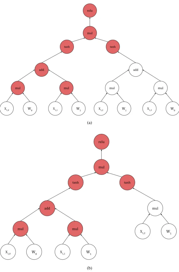
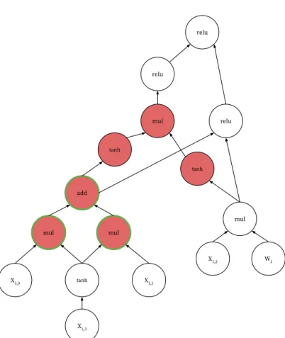
Recent research shows that such models may have excellent performance if structural informa-tion of input data can be captured by their representainforma-tions. The aforemeninforma-tioned Tree-LSTM model is one such data-dependent model. An example of two DAGs built on different data inputs with the same model weights is shown in Figure 3.1. From this figure, we can see that the example in
Figure 3.1a contains 4 words in the input sentence (X1,0toX1,3), thus forming a computation DAG
with 18 nodes, including 8 input nodes and 10 operators. The Example in Figure 3.1b contains 3 words (X2,0 toX2,2) in the input sentence and forms a computation DAG with 14 nodes, including
6 input nodes and 8 operators. Different structure in the computation DAGs make it impossible for the deep learning system to directly apply uniform optimizations that apply for every piece of input data.
3.3 PROBLEM DEFINITION
With the definition of the notation we use concluded, we can now formally describe our problem: Problem 3.1. Given a deep learning training loopL containing 1) a data dependent model M
with model weight setW ={wi}, and 2) a training dataset organized in batches of examplesB =
{bi}, we want to minimize the total runtime ofT(L)(defined as T(L) =
P|B|
i=1(T(M(Wi, Bi)) +
X1,0 W0 mul add X1,1 W1 mul tanh X1,2 W1 mul add X1,3 W0 mul tanh mul relu (a) X1,0 W0 mul add X1,1 W1 mul tanh X1,2 W1 mul tanh mul relu (b)
CHAPTER 4: DETECTING AND LEVERAGING FREQUENT SUBGRAPHS
Given the fact that it is inefficient to optimize every computation DAG induced by training examples, a natural alternative could involve finding common execution patterns contained in dif-ferent DAGs. These common subgraphs could be optimized a single time, and each time such a pattern is detected in the training example, the optimized variant could then be applied. For exam-ple, the red-colored nodes in Figure 3.1 depect an execution pattern common to both computation DAGs. A typical compiler optimization technique known as common subexpression elimination
(CSE) tries to replace the frequently- occurring expressions in code with a temporary variable. By analogy, we might also have similar effect after substituting a frequently-occurring subgraph in DAGs with an alternative optimized variant. The optimized subgraph will take the same input as the original subgraph and yield identical output.
4.1 FREQUENT SUBGRAPH PATTERN DETECTION
We can more formally describe our frequent subgraph detection task as follows. Given a set S ={Gi}containing input data DAGs, we need to 1) detect some frequent subgraphsS0 ={G0i}
and 2) for eachG0i ∈ S0 we need to provide an optimized versionG+i . A subgraph patternG0 is marked as frequent in DAG setSwhen the number of total occurrence ofG0divided by the size of Sis greater than some predefined threshold valuePF req.
The second subtask is much easier to tackle since, given a graph representation, we will always be able to use domain knowledge to change the order of execution or rewrite a sequence of opera-tors into some more efficient representation. The aforementioned APIs in TensorFlow Eager and PyTorch can automate the optimization process and generate a good enough alternative subgraph. Although there is no guarantee that we can always achieve the best runtime using this compilation tool, the performance is satisfactory, as we will demonstrate with experiments regarding perfor-mance oftf.contrib.eager.defun(Section 6.2).
The first subtask is considerably more difficult. This is because detecting whether a particular subgraph occurs (either for assessing frequency or for applying an optimized variant) is exactly the subgraph isomorphism problem, which is NP-Complete for DAGs (since general subgraph
isomorphism is NP-Complete [12] — consider the straightforward reduction whereby each edge (a, b) is replaced by a new nodecwith an edge toa and an edge tob). Thus, without additional restrictions on the subgraphs we detect, it’s likely that the cost of pattern searching will swallow any benefit brought by just-in-time compilation.
A further difficulty stems from the data-dependent aspect of our problem. The popular frame-works that support data-dependent models are define-by-run; but, if we do not know the “defini-tion” (i.e., the graph structure) until the model is actually run, then there is no point of applying further optimizations since we have already run the model. Therefore, a major challenge is to instrument the typical user-provided define-by-run code so that graph structures can be extracted without explicitly running the model.
4.2 DAG EQUIVALENCE
Before we can detect frequent subgraphs in different computation DAGs, we first define different levels of equivalence between two DAGs. Because each training example may contain different information, it is unrealistic to require two DAGs representing the computation of different input data to be completely identical in terms of content. We discuss three different notions for DAG equivalence here, and we determine which equivalence will be most suitable to our target scenarios. Shape Equivalence.Our first notion equivalence is the strictest. Given two DAGsG1 = (N1, E1)
andG2 = (N2, E2), we consider them to beequivalent in shapewhen the following two conditions
are satisfied:
1. The output node ofG1 has same Tensor shape and operator as the output node ofG2.
2. For every pair of nodes(ni, nj)withni ∈N1andnj ∈N2with the same shape and operator,
letPk(x)denotes the k-th input of nodex. ThenPk(ni)andPk(nj)must have same shape
and same operator, for all0≤k < len(Pk(ni)).
Structure Equivalence. Shape equivalence, which is the strongest notion used for comparing two DAGs, might be impractical when a model takes inputs with different shapes but has the same processing logic. Structure equivalence has a similar definition to that of shape equivalence but relaxes the requirement of identical Tensor shape. Two nodes are consider equivalent in structure
when their corresponding input nodes are equivalent in structure and they have same operator. This definition of equivalence reduces the number of possible distinct subgraphs. In practice, however, it is still expensive to compare each node in two graphs efficiently.
Signature Equivalence. Signature equivalenceis even weaker than structure equivalence in that it provides a simple representation for every subgraph. A subgraph rooted at node ni can be
represented with a series of hashed strings. Two subgraphs are considered equivalent in signature when they share the same hashed string representation, which we elaborate on below. Consider a hash functionH(x)and a node ni with operator fi, and let Pk(ni)be thekth input node of ni.
DefineH(ni)as
H(ni) = H(fi, H(P0(ni)), ..., H(PL−1(ni)))
whereLis the number of inputs ofni. That is, two subgraphs share the same hash signature if they
have the same operator and if their inputs share the same respective hash signatures. This recursive definition of subgraph signatures reaches the end when the node is a leaf node (input node) in the computation DAG. We set each leaf nodenleaf’s signature to a predefined constant valueC. One
benefit of this subgraph encoding is that during the hash computation, the node’s encoded value can be shared between multiple depending nodes, thereby avoiding significant computation.
4.3 DAG STRUCTURE CONSTRUCTION BEFORE EVALUATION
After defining various notions of equivalence and showing how signature equivalence gives an efficient way to represent DAGs, we are now able to search and record subgraph occurrences in a given computation DAG. However, since the DAG is built at runtime, we also need to separate the DAG construction process from the actual DAG evaluation. In deep learning frameworks like PyTorch and TensorFlow, these occur together by default, so preserving existing APIs while teasing apart these two processes is a major challenge. We address this by constructing a lazily-evaluated DAG (referred to as a lazy DAG) identical to the computation DAG built during eager evaluation. To achieve this, we usemonkey patchingto replace the Tensor operator APIs used in user programs with our own operator recording APIs. We will describe in Section 5.2 how this monkey patching is implemented so that existing user code requires minimal to no modifications.
4.4 REVISED PATTERN REPRESENTATION
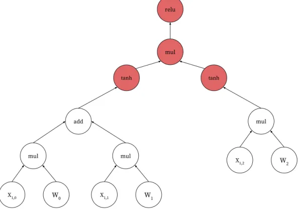
In the discussion about signature equivalence in Section 4.2, we showed how to recursively apply our hashing strategy starting at the root node and expanding until we reach the leaf nodes of original DAG. Under this representation, we are not able to detect patterns that end at non- leaf nodes. To solve this, we now give a revised representation of subgraph signature that enforces a maximum depth. LetH0(n, d)denote the signature of subgraph starting at nodenwith a maximum depth of d. Under this definition, we will always setH0(n,0)to some predefined constant value C. Using this representation, internal subgraphs can also be represented efficiently, albeit at some cost in the flexibility in the types of subgraphs can be respresented. Figure 4.1 shows a example of subgraph with depth = 2 inside a computation DAG ending with non-leaf nodes.
X1,0 W0 mul add X1,1 W1 mul tanh X1,2 W2 mul tanh mul relu
4.5 SUBGRAPH PATTERN SEARCH STRATEGY
After we are able to encode subgraphs with a specified depth limit, we can start searching for subgraphs in a computation DAG. We use a queueQto perform the subgraph match. Given a set of subgraph signaturesS ={si}and a computation DAGG, we first push the root node ofGinto
Q. As long asQis non-empty, we pop the head nodenh ofQ. We perform a subgraph encoding
starting fromnh with maximum depth equal toPDepth (a user-controlled parameter). IfPDepth is
too small, we may find trivial patterns that are not worth optimizing; ifPDepthis too large, it may
be difficult to find frequent subgraphs. The subgraph encoding function will return the signature of the subgraph as well as a list containing all input nodes of that subgraph. These aforementioned inputs are then pushed ontoQ. We compare the resulting signature with each signature present in S. If the signature matches one of the signature in the setS, we claim that we found the subgraph pattern. The search on the DAGGterminates whenQis empty.
4.6 SUBGRAPH REPLACEMENT
Every time we match a frequent subgraph signature in a DAGG, we will replace this subgraph with a single special operator. Denote the root node (which is also the output node) of a subgraph G0 byno, and denote the set of input nodes ofG0 byG0in. We will rewrite the DAGGby directly
connecting no with all the nodes in G0in. The operator of no will also be replaced by a special
operator specifying the corresponding signature. Later, this operator will be just-in-time compiled once, after which all occurrences can use the optimized version.
4.7 FULL ALGORITHM
Now we demonstrate a complete algorithm that combines all the techniques described above. The algorithm consists of two stages:
1. The frequent pattern collecting stage, and 2. the DAG optimization stage.
Stage 1: Pattern Collection. In the first stage, our framework will use the subgraph encoding function to collect occurrences of subgraphs in DAGs of the firstPCollecttraining batches (where
PCollect is a user-provided paramter). After the first stage, our framework will filter our patterns
with frequency below some minimum occurrence thresholdPF req (another parameter).
Stage 2: DAG Optimization. In the DAG optimization stage, for every computation DAG of the input data, we match and substitute the frequent subgraphs in the DAG with previously-mentioned special operators from Section 4.6. After we optimize the DAG corresponding to a piece of input data, we then trigger the evaluation of the DAG. The DAG evaluation will be executed recursively by an executor function, starting from the root node until it reaches leaf nodes (which correspond either to input data or to model weights). A node ni can be computed only when all its children
are computed. This computation is performed by applying ni’s own operator on its children’s
computed values. When the DAG executor encounters a node with an operator indicating that it is an optimized subgraph operator, the executor will check if our framework has cached an optimized function corresponding to this subgraph. If present, the executor will apply the optimized function. Otherwise, the executor will generate the optimized function equivalent to the logic of subgraph and store it for future use. Thus, subgraphs with identical signatures will only be optimized once during execution.
4.8 LIMITATIONS
Our approach has a few limitations. First, our algorithm can only detect subgraphs with the same maximum depth. It cannot generate and detect subgraph patterns with arbitrary shapes. Therefore, we could fail to detect “better” frequent subgraphs using this approach. Second, the subgraph patterns detected by our algorithm are not very interpretable. Thus, the detected patterns are unlikely to be related to the model structure, should the user choose to inspect them.
CHAPTER 5: FRAMEWORK IMPLEMENTATION
In Section 4.7 we described our high-level algorithm for efficient detection, optimization, and application of frequent subgraphs in data-dependent computation DAGs. In this chapter we de-scribe the specific implementation details of our framework. We will first introduce thecontext manager, which is the core component of our framework, and we will show how we implement our algorithm on top of our framework. We implement our framework in the Python language and build it on top of TensorFlow Eager mode. Although we choose TensorFlow Eager as our first target, we believe that our implementation can be easily ported to PyTorch.
5.1 CONTEXT MANAGER
In this section we describe the core part of our framework, which is the context manager. A context manager is a single class object in our framework which monitors and stores all the global information of our framework. The context manager contains information and data structures related to:
1. object tracking,
2. frequent pattern signatures and optimized function representations, 3. session information in pattern searching, and
4. user-controlled global parameters.
This context manager is included in our framework so that when users import our framework’s package in their code for the first time, the context manager will be created automatically.
Object Tracking.The object tracking is a crucial part in the context manager. The object here are divided into four types:
1. TensorFlowEagerTensors, which should be input data value types in the input example. 2. ints and floats, corresponding to constant value used as parameters in some TensorFlow
3. TensorFlowVariables, corresponding to model weights used in the computation DAG. 4. Virtual Nodes, instantiations of a framework-defined data structure used in our lazy DAG
abstraction.
Each object is assigned a unique global id so that the framework can track them efficiently. Object tracking is implemented in the following way. Every time the framework receives or constructs an object obj, it will call get gid(obj)to locate the global id (referred as gid) of the object to see if this object already exists in context manager. If not found, the manager will assign a new global idgidobj. The context manager will establish a bi-directional mapping:
id(obj)−→gidobjandgidobj−→obj. Having this two-way indexing allows the framework to perform efficient node lookups during DAG construction and optimization. The indexing incurs only a small amount of extra memory cost as it only storesreferences of original objects but not
full copies.
Frequent Pattern Management. The second function provided by the context manager is the ability to keep track of all the information about detected frequent subgraphs. The context manager keeps a counter of the number of occurrences for every DAG signature encountered during the frequent pattern collecting stage. It uses this to filter out patterns that are below user defined frequent threshold. For every frequent pattern, the context manager also stores the number of input nodes and a function object consisting of a sequence of TensorFlow operations reflecting the logic of the optimized subgraph. When evaluating the computation DAG, if a node is encountered with an operator representing an optimized subgraph computation, the context manager will feed the operator’s function object to the DAG executor, which compiles and caches optimized operators for later use (ensuring that identical subgraph patterns will only incur optimization overhead once). Session Information. Sessions are used in our framework to refer to a single pattern search pro-cess. Nodes in computation DAGs that are visited during a given session will be tagged with an identifier unique to the session. The context manager also possesses a session constant object tracker that will be used to detect leaf nodes in subgraphs, which will help avoid duplicate leave nodes in subgraph searching.
Parameters. There are some other algorithm-related parameters stored in the context manager whose defaults may be overwritten by framework users, such as the aforementioned pattern
fre-quency thresholdPF req. In our current implementation, users are allowed to modify these
param-eter values by calling the framework’s helper functionset parameter(key, val).
5.2 DAG CONSTRUCTION
TensorFlow Eager mode evaluates the computation DAG for each training example at the same time it builds the example’s computation DAG, as all the operators are eagerly evaluated. As mentioned in Section 4.3, we need to separate the DAG construction and evaluation via a lazy evaluation approach. Our framework achieves this by introducing theVirtual Nodedata structure. With the help of this Virtual Node, our framework can obtain the example’s computation DAG structure without performing any actual computation. In this section, we will first describe the Virtual Node data structure, and after which we describe how to use monkey patching to substitute the original user-specified TensorFlow operators with our own Virtual Nodes.
Virtual Nodes.TheVirtual Nodedata structure is designed to represent any TensorFlow operator. A Virtual Node object is a node in our constructed computation DAG that contains the following main components:
1. op: Name of TensorFlow operator;
2. arg ids: A list that containsgidof its input nodes in the DAG; and
3. dep nodes: A list that contains thegids of nodes that take this node as one of their inputs. Other components are omitted in our description. By tracing Virtual Nodes and leveraging the information stored therein, the computation DAG for the original TensorFlow code representing the user’s the model logic can be reconstructed during the DAG evaluation stage.
Monkey Patching. To capture the user-defined model logic without actually running it, we fa-cilitate lazy evaluation via tracinguser code. If we want to keep the user’s code untouched, we need to place the tracer inside TensorFlow’s APIs, which requires a huge amount of work and is sensitive to changes due to version updates in TensorFlow.
A useful technique is monkey patching. Monkey patching is a technique that enables a program to modify or extend its behavior locally. Notice that deep learning code defined in TensorFlow Eager that includes an addition of two Tensors can be abstracted as:
i m p o r t t e n s o r f l o w a s t f . . . # t f . add ( ) i s a T e n s o r F l o w o p e r a t o r t o # add t w o T e n s o r s w i t h same d i m e n s i o n s . o u t = t f . add ( i n 1 , i n 2 ) . . .
For all the TensorFlow API functions used to define models definition, we can define correspond-ing functions in our framework that take the same number of inputs and generate same number of outputs. Here is an example of composing tf.add(x, y) with our own framework’s lazy variant:
d e f add ( x , y ) :
# S p e c i f y t h e o p e r a t o r t y p e and i n p u t a r g u m e n t s # ’ add ’ m u s t m a t c h t h e ’ add ’ i n ’ t f . add ’
r e t = V i r t u a l N o d e ( ’ add ’ , 2 , [ x , y ] ) # S e t g l o b a l i d f o r r e t u r n o b j e c t r e t . s e t g i d ( c t x . g e t g i d ( r e t ) ) # Add d a t a d e p e n d e n c i e s b e t w e e n i n p u t n o d e s and o u t p u t n o d e r e t . s e t a r g s d e p ( ) r e t u r n r e t
Thectxin the above code block is the instance of framework’s context manager. Now our frame-work can trace the model’s computation logic by swapping the import for TensorFlow with that of our own framework. After DAG construction, the user can evaluate the DAG and get the output with thebuild(out)function, whereoutis the output node of the DAG.
# i m p o r t t e n s o r f l o w a s t f i m p o r t t r a c e r a s t f . . . # t f . add ( ) i s monkey−p a t c h e d o u t = t f . add ( i n 1 , i n 2 ) . . .
# b u i l d ( ) e v a l u a t e s t h e DAG c o n s t r u c t e d by V i r t u a l Nodes , # w h i c h p e r f o r m s t h e a c t u a l c o m p u t a t i o n . i f h a s a t t r( t f , ’ b u i l d ’ ) : r e s u l t = t f . b u i l d ( o u t ) e l s e : r e s u l t = o u t . . .
Our implementation has the advantage that users can apply our optimization by merely swapping library imports and adding a few lines for DAG evaluation.
Limitation. Our problem definition and implementation assumes that any operator in our compu-tation DAG takes one or more inputs and generates exactly one output. Most of the TensorFlow APIs satisfy this condition with a few notable exceptions, such astf.split(). tf.split() is a TensorFlow operator that splits an input Tensor into multiple output Tensors. The number of outputs is determined by an input argumentnum or size splits. In order to resolve this, our framework introduces an extra function namedaccess(x, i)which returns theith value of a listx. This extra function adds an extra node (and operation) in the DAG construction.
5.3 PATTERN SEARCHING
In this section we describe some details in our implementation that help accelerate the pattern searching and future optimization process. During pattern searching, some nodes might be visited multiple times. A natural thought is to expand the DAG, so that some nodes will show up multiple times in a subgraph. However, if a subgraph is large enough, a large portion of nodes will be duplicated, which will largely increase the number of input arguments of the optimized function for this subgraph and increase the runtime of the optimized function, which is an undesirable result.
To solve this, we append a session tag to each node during pattern search. At the beginning of each pattern search, a new session is created and assigned a unique session tags. When the pattern search function encounters a node with no session tag or with a session tags0 not equal to that of this sessions, this means that it is the first time this node has been visited in our session, and we
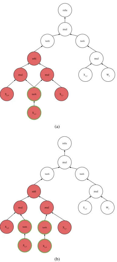
X1,0 tanh mul add X1,1 mul tanh X1,2 W2 mul tanh mul relu X1,3 (a) X1,0 tanh mul add X1,1 mul tanh X1,2 W2 mul tanh mul relu X1,3 tanh X1,4 (b)
assignsto its session tag. When our search function encounters a nodenwith the same session tag s, it will not proceed to traverse the children ofnfor the second time; instead, its signature will be H(shared(H(n))). A simplified example of this shared subgraph is shown in Figure 5.1. Using a wrapper stringshared()in the hash signature computation prevents the DAG in Figure 5.1a from having the same signature as that in Figure 5.1b. The pattern in Figure 5.1a will be
H(add, H(mul, H(C), H(tanh, H(C))), H(mul, H(shared(H(tanh, H(C)))), H(C)))
while the pattern in Figure 5.1b will be
H(add, H(mul, H(C), H(tanh, H(C))), H(mul, H(tanh, H(C)), H(C)))
Note that the hash value insideshared()is reused, thereby avoiding extra computation.
5.4 SUBGRAPH OPTIMIZATION
After we verify that a subgraph is frequent and decide to optimize it, DAG translation is needed to transform the subgraph representation back to TensorFlow code. We will first introduce our
code generationprocedure, and then we will describe how to optimize the translated TensorFlow code snippet.
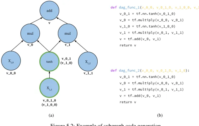
Subgraph Code Generation. During the frequent pattern collecting stage, we do not perform any subgraph code generation and optimization. In the DAG optimization stage, when we find a subgraph rooted at nodenthat is frequent and has not been optimized, we will perform a subgraph traversal fromnto generate the code.
The logic of traversal is as follows. Starting fromn, we mark the output variable ofn in code asv. The variable names of the children ofn will bev 0, v 1, v 2and so on. Similarly, the input ofv 1will bev 1 0, v 1 1 and so on. We will perform a depth-first traversal on the nodes in the subgraph until we reach the input nodes (leaves). Starting from these input nodes, the DAG can be transformed back to TensorFlow operators line-by-line.
Figure 5.2 depicts an example of subgraph translation in which two nodes in the same subgraph are reused. According to the naming logic in our code generation, each of these nodes can have two
X1,0 tanh mul add X1,2 mul X1,1 v v_0 v_1 v_0_0 v_0_1 (v_1_0) v_0_1_0 (v_1_0_0) v_1_1 (a) def dag_func_1(v_0_0, v_0_1_0, v_1_0_0, v_1_0): v_0_1 = tf.nn.tanh(v_0_1_0) v_0 = tf.multiply(v_0_0, v_0_1) v_1_0 = tf.nn.tanh(v_1_0_0) v_1 = tf.multiply(v_0_1, v_1_1) v = tf.add(v_0, v_1) return v def dag_func_2(v_0_0, v_0_1_0, v_1_0): v_0_1 = tf.nn.tanh(v_0_1_0) v_0 = tf.multiply(v_0_0, v_0_1) v_1 = tf.multiply(v_0_1, v_1_1) v = tf.add(v_0, v_1) return v (b)
Figure 5.2: Example of subgraph code generation
variable names (since these nodes are reachable via two separate paths during traversal). One way of dealing with this is to separate these nodes into two copies. In this case, thetanhnode will have two copiesv 0 1andv 1 0, andX1,1will have two copiesv 0 1 0andv 1 0 0. The generated
function looks likedag func 1in Figure 5.2b which takes 4 input arguments and is composed of 5 TensorFlow operations. When the computation DAG is large enough, it is likely that multiple subgraphs are detected to be optimized, in which case this implementation will introduce a great amount of unnecessary computation and memory cost. To alleviate this, our implementation keeps track of nodes that have been visited and their variable names. If a node is marked as visited during traversal, our code will use the variable name it was assigned previously. The updated generated function is given by dag func 2 in Figure 5.2b. In this function, the tanh node is uniformly referred to asv 0 1on each occurrence.
Function Optimization. We optimizate the code generated for a given subgraph using just-in-time (JIT) compilation. For TensorFlow, this simply amounts to using the graph compilation API f0 =tf.contrib.eager.defun (f). By callingdefun the with generated code, Tensor-Flow will build a graph for the TensorTensor-Flow operations present in this function return an optimized
version. The context manager will cache this optimized function for use with future occurrences of signature-equivalent subgraphs.
5.5 AVOIDING EXTRA COMPUTATION
Another issue in DAG optimization and DAG evaluation is that nodes can be computed multiple times during optimization if we are not careful. In Figure 5.3, which depicts a simplified example of extra computation, the red nodes correspond to a frequent pattern that has been optimized. If computation of the red subgraph is completed via the optimized generated function, which is unaware of duplicate computation, then the nodes with green borders could be computed twice (since theaddnode with a green border is a dependency for therelunode on the right, in addition to being part of the optimized subgraph). During our preliminary testing, we found out that this sort of extra computation will offset many of the benefits brought by subgraph optimization and slow down model training time significantly.
In our implementation, we thus add a constraint to avoid this scenario. If a noden is used by more than one node in the computation DAG, this node should not be a node in any optimized subgraphunlessit is the root or a leaf of the subgraph. This constraint ensures that all dependents of non-root nodes belonging to an optimized subgraph will only be present in the subgraph, thereby avoiding the pathological extra computation.
X1,0 tanh mul add X1,1 mul tanh X1,2 W2 mul tanh mul relu X1,3 relu relu
CHAPTER 6: EVALUATION
6.1 EXPERIMENT SETTINGS
Environment. We performed all of our experiments on a computer with single Intel Core i7 CPU. We did not conduct any GPU experiments, but we believe that our framework would yield similar results in such a setting. We use Python version 2.7.15 and implemented models using TensorFlow version 1.12.0.
Datasets. In our experiments we used two open source datasets. The first one is the MNIST [17] dataset, which can be imported fromtensorflow.python.keras.datasets. This dataset contains 60000 hand-written digit images, each of which is comprised of a 28×28 grid of pixels. We used the MNIST dataset to train multiple classification models.
The second dataset we used is the Stanford Sentiment Treebank (SST) dataset [18]. SST con-tains fine-grained sentiment labels for 215154 phrases in the parse trees of 11855 individual sen-tences extracted from movie reviews. This dataset is a common benchmark for sentiment analysis tasks. As suggested in [10], we used 6920 training sentences for binary sentiment classification. Model Descriptions. In our experiments we used several well-known deep learning models. We will describe how we implemented these models in TensorFlow Eager mode, the parameters for each model, and the purpose of using these models.
Convolutional Neural Networks (CNNs). Convolutional nets [19] have been widely used on vision tasks like image classification. For MNIST digit recognition, we implement a simple CNN model with two convolutional layers with3×3kernels, one pooling layer, and one dense layer. The batch size is set to 128.
Recurrent Neural Networks (RNNs). Recurrent nets [20] use internal state to process a sequence of inputs. Recurrent architectures are also applicable to tasks like hand-written digit recognition. We implement a simple RNN with two layers of 128-unit LSTM cells. The batch size is 100. Bidirectional Recurrent Nueral Nettworks (Bi-RNNs). The bidirectional recurrent architec-ture [21] is a variant of the RNN architecarchitec-ture that connects two hidden layers from an original sequence and a reversed sequence to the same output. We implement our Bi-RNN model with the same parameters as for the previous RNN model.
Tree-LSTMs. The Tree-LSTM model [10] is a variant of the LSTM model [22]. Tree-structured LSTMs diverge from the original LSTM model in that information is propagated recursively in a tree shape induced by the input data as opposed to sequentially. We implement the Tree-LSTM model for a sentence-level binary sentiment classification task, using sentences from SST. For each input sentence, a constituency binary parse tree is provided. We implement our Tree-LSTM model with embedding dimension of 300, hidden dimension of 150, dropout rate = 0.5, regularization = 0.0001 and batch size = 20.
6.2 GRAPH COMPILATION OPTIMIZATION EXPERIMENTS
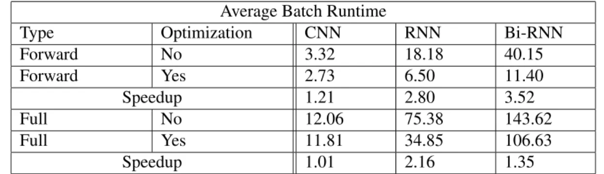
In this section, we will demonstrate the performance of TensorFlow’s graph optimization tool tf.contrib.eager.defunon the first three models. Since these three models are all data-independent models, only one type of computation DAG will be generated. As such, it will be easy to apply graph optimization on these models. Since we build these three models on topic of the Keras API, applying defun optimization on each model can be as easy as tagging the model.call()method with [email protected]. For each model, we run on the MNIST data with two types: 1) Only forward pass computation, and 2) Forward pass and backward pass computation. The average times taken for each model to execute a batch with different execution settings are shown in Table 6.1.
Average Batch Runtime
Type Optimization CNN RNN Bi-RNN
Forward No 3.32 18.18 40.15 Forward Yes 2.73 6.50 11.40 Speedup 1.21 2.80 3.52 Full No 12.06 75.38 143.62 Full Yes 11.81 34.85 106.63 Speedup 1.01 2.16 1.35
Table 6.1: Result of manually applying graph optimization on different models.
From the table we can see that simply adding graph optimization to a model’s forward pass logic can have a large performance gain. The CNN model has the least performance speedup among all three models. The RNN and Bi-RNN models both achieve more than 2.8× speedup when
per-forming only forward computation. It can be concluded from the table that performance speedups increase when the model logic becomes more complex, because complex models can have larger computation graphs (and therefore more TensorFlow operations), providing more potential bene-fits from the application of graph optimizations.
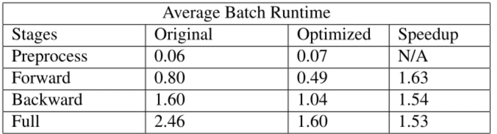
6.3 MANUAL PATTERN OPTIMIZATION EXPERIMENT
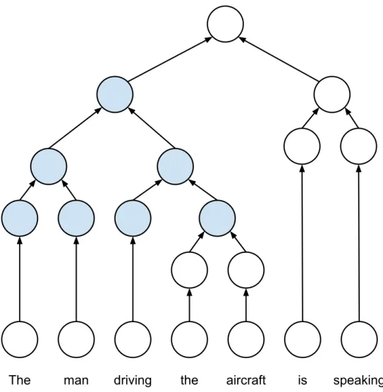
In this section we demonstrate the performance gain of manually applying a graph optimization technique to on a specific subgraph pattern encountered during training of a data-dependent model: the Tree-LSTM model. This model was implemented for a sentence-level binary sentiment clas-sification task. The Tree-LSTM architecture is more complicated than those of the previous three models as it involves more TensorFlow operations for every node in a given input parse tree. With domain knowledge, we search for a simple subgraph pattern that involves seven parse tree nodes (in the shape of a complete binary tree). An example of this pattern on a parse tree of a sentence is shown in Figure 6.1.
To implement pattern matching on the eagerly evaluated model, we introduce lazy evaluation in this model’s implementation. Traversing children nodes will return some metadata that helps a node to decide whether the desired pattern was found and if it is suitable for optimization. We run both the original and optimized variants of the Tree-LSTM implementations on the Stanford Sen-timent Treebank dataset for 5 epochs and compute the average batch runtime statistics. Detailed results are provided in Table 6.2.
Average Batch Runtime
Stages Original Optimized Speedup
Preprocess 0.06 0.07 N/A
Forward 0.80 0.49 1.63
Backward 1.60 1.04 1.54
Full 2.46 1.60 1.53
Table 6.2: Result of manually applying graph optimization on Tree-LSTM model.
From the table we can see that applyingdefunto occurrences of our provided pattern can give considerable reductions in runtime. The Tree-LSTM architecture runs slowly since each example
The man driving the aircraft is speaking
Figure 6.1: Example of manual pattern optimization
with a different computation DAG structure is executed sequentially, so the 1.53× speedup is considered fairly substantial.
6.4 FRAMEWORK OPTIMIZATION EXPERIMENT
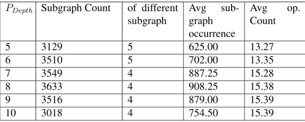
Finally, we test the performance of our framework on Tree-LSTM. As mentioned in the previous chapters, our framework provides user-controlled parameters PDepth, PF req, and PCollect. Before
we execute our full algorithms, we should first tuned these parameters. We setPCollect to 3, as we
believe that three batches containing around 1%of total training examples should be enough for frequent subgraph collecting We first setPF req to 1 (which means the detected subgraphs occurs
of different subgraphs and their occurrences. The results are shown in Table 6.3.
PDepth Subgraph Count of different
subgraph Avg sub-graph occurrence Avg op. Count 5 3129 5 625.00 13.27 6 3510 5 702.00 13.35 7 3549 4 887.25 15.28 8 3633 4 908.25 15.38 9 3516 4 879.00 15.39 10 3018 4 754.50 15.39 Table 6.3: Result
From the table we can see that, when PDepth = 8, the number of subgraphs detected by our
framework reaches is maximized (when considering the first 60 examples). We thus use this value in our final experiment.
The average batch execution time under our framework and for the original version are given in Table 6.4.
Average Batch Runtime
Stages Original Optimized Speedup
Preprocess 0.09 0.09 N/A
Forward
DAG Construction 0.39 0.41 N/A
Optimization 0.00 0.18 N/A
Execution 0.87 0.45 1.93
Total 1.26 1.04 1.21
Backward 1.62 1.08 1.50
Full 2.97 2.20 1.35
Table 6.4: Result of automatically applying graph optimization on Tree-LSTM model.
The original baseline in table Table 6.4 refers to Tree-LSTM model used with our framework and no pattern searching is involved. From the table we can see that our pattern searching algo-rithm achieved 1.35×speedup on Tree-LSTM model.The speedup is not as good as the manually optimized version because of the additional framework-introduced overhead involved in building the computation DAG and searching for possible subgraph patterns. The building of computation DAGs takes about 0.4 seconds per batch when using our framework. We believe that this overhead comes from creating hundreds of Virtual Nodes when building the computation DAG, and it can
definitely be optimized away in the future if memory can be pre-allocated in our future frame-work implementation. The pattern searching algorithm in our frameframe-work makes no guarantees that the subgraph patterns that provide the largest speedups via graph optimization will necessarily be found. One can expect that the total runtime speedup can be improved with a more sophisti-cated pattern searching algorithm, and perhaps with additional framework-specific implementation optimizations.
CHAPTER 7: CONCLUSION
In this thesis, we presented a hashing based frequent subgraph search algorithm that is able to detect and optimize computation logic shared across different computation graphs. Our algorithm includes efficient techniques for testing subgraphs equivalence as well as lightweight frequent sub-graph detection and optimization. We implemented our detection framework on top of TensorFlow and provided several optimizations used to avoid extra computation during execution. We show that our framework’s implementation can be integrated into user programs seamlessly with nearly zero code changes. Our experiments on the Stanford Sentiment Treebank dataset show that, when used to optimize the Tree-LSTM model, our algorithm is able to detect non-trivial frequent pat-terns on real data and is1.35×faster than an unoptimized Tree-LSTM implementation, suggesting that such fine-grained workflow optimization techniques could lead to further benefits when used in the context of deep learning frameworks.
REFERENCES
[1] A. Paszke, S. Gross, S. Chintala, G. Chanan, E. Yang, Z. DeVito, Z. Lin, A. Desmaison, L. Antiga, and A. Lerer, “Automatic differentiation in pytorch,” 2017.
[2] M. Abadi, P. Barham, J. Chen, Z. Chen, A. Davis, J. Dean, M. Devin, S. Ghemawat, G. Irving, M. Isard et al., “Tensorflow: A system for large-scale machine learning,” in12th{USENIX}
Symposium on Operating Systems Design and Implementation ({OSDI}16), 2016, pp. 265– 283.
[3] J. Dean and S. Ghemawat, “Mapreduce: simplified data processing on large clusters,” Com-munications of the ACM, vol. 51, no. 1, pp. 107–113, 2008.
[4] M. Zaharia, M. Chowdhury, M. J. Franklin, S. Shenker, and I. Stoica, “Spark: Cluster com-puting with working sets.”HotCloud, vol. 10, no. 10-10, p. 95, 2010.
[5] D. Xin, L. Ma, J. Liu, S. Macke, S. Song, and A. G. Parameswaran, “Accelerating human-in-the-loop machine learning: Challenges and opportunities,” in Proceedings of the Second Workshop on Data Management for End-To-End Machine Learning, DEEM@SIGMOD 2018, Houston, TX, USA, June 15, 2018, 2018. [Online]. Available: https://doi.org/10.1145/3209889.3209897 pp. 9:1–9:4.
[6] T. Chen, M. Li, Y. Li, M. Lin, N. Wang, M. Wang, T. Xiao, B. Xu, C. Zhang, and Z. Zhang, “Mxnet: A flexible and efficient machine learning library for heterogeneous distributed sys-tems,”arXiv preprint arXiv:1512.01274, 2015.
[7] R. Al-Rfou, G. Alain, A. Almahairi, C. Angermueller, D. Bahdanau, N. Ballas, F. Bastien, J. Bayer, A. Belikov, A. Belopolsky et al., “Theano: A python framework for fast computa-tion of mathematical expressions,”arXiv preprint arXiv:1605.02688, 2016.
[8] D. Xin, S. Macke, L. Ma, J. Liu, S. Song, and A. Parameswaran, “Helix: Holistic opti-mization for accelerating iterative machine learning,”Proceedings of the VLDB Endowment, vol. 12, no. 4, pp. 446–460, 2018.
[9] N. P. Jouppi, C. Young, N. Patil, D. Patterson, G. Agrawal, R. Bajwa, S. Bates, S. Bhatia, N. Boden, A. Borchers et al., “In-datacenter performance analysis of a tensor processing unit,” in2017 ACM/IEEE 44th Annual International Symposium on Computer Architecture (ISCA). IEEE, 2017, pp. 1–12.
[10] K. S. Tai, R. Socher, and C. D. Manning, “Improved semantic representations from tree-structured long short-term memory networks,”arXiv preprint arXiv:1503.00075, 2015. [11] M. Looks, M. Herreshoff, D. Hutchins, and P. Norvig, “Deep learning with dynamic
compu-tation graphs,”arXiv preprint arXiv:1702.02181, 2017.
[12] S. A. Cook, “The complexity of theorem-proving procedures,” in Proceedings of the third annual ACM symposium on Theory of computing. ACM, 1971, pp. 151–158.
[13] M. Zaharia, M. Chowdhury, T. Das, A. Dave, J. Ma, M. McCauley, M. J. Franklin, S. Shenker, and I. Stoica, “Resilient distributed datasets: A fault-tolerant abstraction for in-memory clus-ter computing,” inProceedings of the 9th USENIX conference on Networked Systems Design and Implementation. USENIX Association, 2012, pp. 2–2.
[14] X. Meng, J. Bradley, B. Yavuz, E. Sparks, S. Venkataraman, D. Liu, J. Freeman, D. Tsai, M. Amde, S. Owen et al., “Mllib: Machine learning in apache spark,”The Journal of Machine Learning Research, vol. 17, no. 1, pp. 1235–1241, 2016.
[15] J. Andreas, M. Rohrbach, T. Darrell, and D. Klein, “Learning to compose neural networks for question answering,”arXiv preprint arXiv:1601.01705, 2016.
[16] G. Neubig, Y. Goldberg, and C. Dyer, “On-the-fly operation batching in dynamic computa-tion graphs,” inAdvances in Neural Information Processing Systems, 2017, pp. 3971–3981. [17] Y. LeCun, “The mnist database of handwritten digits,”http://yann. lecun. com/exdb/mnist/. [18] R. Socher, A. Perelygin, J. Wu, J. Chuang, C. D. Manning, A. Ng, and C. Potts, “Recursive
deep models for semantic compositionality over a sentiment treebank,” inProceedings of the 2013 conference on empirical methods in natural language processing, 2013, pp. 1631–1642. [19] A. Krizhevsky, I. Sutskever, and G. E. Hinton, “Imagenet classification with deep convo-lutional neural networks,” inAdvances in neural information processing systems, 2012, pp. 1097–1105.
[20] T. Mikolov, M. Karafi´at, L. Burget, J. ˇCernock`y, and S. Khudanpur, “Recurrent neural net-work based language model,” inEleventh annual conference of the international speech com-munication association, 2010.
[21] M. Schuster and K. K. Paliwal, “Bidirectional recurrent neural networks,”IEEE Transactions on Signal Processing, vol. 45, no. 11, pp. 2673–2681, 1997.
[22] S. Hochreiter and J. Schmidhuber, “Long short-term memory,”Neural computation, vol. 9, pp. 1735–80, 12 1997.