Chapman University Chapman University
Chapman University Digital Commons
Chapman University Digital Commons
Computational and Data Sciences (Ph.D.)Dissertations Dissertations and Theses
Spring 5-6-2019
Bias Reduction in Machine Learning Classifiers for
Bias Reduction in Machine Learning Classifiers for
Spatiotemporal Analysis of Coral Reefs using Remote Sensing
Spatiotemporal Analysis of Coral Reefs using Remote Sensing
Images
Images
Justin J. Gapper
Chapman University, [email protected]
Follow this and additional works at: https://digitalcommons.chapman.edu/cads_dissertations
Part of the Environmental Indicators and Impact Assessment Commons, Longitudinal Data Analysis and Time Series Commons, Oceanography Commons, and the Statistical Models Commons
Recommended Citation Recommended Citation
J. J. Gapper, "Bias reduction in machine learning classifiers for spatiotemporal analysis of coral reefs using remote sensing images," Ph.D. dissertation, Chapman University, Orange, CA, 2019. https://doi.org/ 10.36837/chapman.000078
This Dissertation is brought to you for free and open access by the Dissertations and Theses at Chapman University Digital Commons. It has been accepted for inclusion in Computational and Data Sciences (Ph.D.)
Bias Reduction in Machine Learning Classifiers for
Spatiotemporal Analysis of Coral Reefs using Remote Sensing Images
A Dissertation byJustin J. Gapper
Chapman University Orange, CA
Schmid College of Science and Technology
Submitted in partial fulfillment of the requirements for the degree of Doctor of Philosophy in Computational and Data Sciences
May 2019
Committee in charge: Hesham El-Askary, Ph.D., Chair
Erik Linstead, Ph.D. Thomas Piechota, Ph.D.
Bias Reduction in Machine Learning Classifiers for
Spatiotemporal Analysis of Coral Reefs using Remote Sensing Images
Copyright © 2019ACKNOWLEDGEMENTS
I would first like to acknowledge and extend my utmost gratitude to the chair of my advisory committee, Hesham El-Askary, Ph.D. Incorporating his original ideas and recommendations were essential to the success of this research. Dr. El-Askary’s constant feedback and encouragement made completing this work possible. In addition, Dr. El-Askary’s work ethic and passion had an immense impact on this work as well as me personally. Finally, I appreciate Dr. El-Askary’s honest candor and insistence on producing only the highest quality scientific research.
I would also like to thank Dr. Linstead and Dr. Piechota for their continual input and support. Dr. Linstead provided valuable feedback on my code and algorithmic approaches for which I am appreciative. Dr Piechota supplied scientific contributions particularly with respect to climatology and providing feedback on responses to journal reviewer comments. I am indebted to and infinitely grateful for my family. First, for the patience and understanding of Judah and Titus during this intense time of work, study, and research. I hope this can be an illustration of perseverance and grit for my sons as they continue to grow and learn. Most of all I want to expound upon the appreciation I have for my beautiful and brilliant wife, Sarah. I want to thank her for her love, support, hard work, and dedication throughout this journey. Sarah and I are an inseparable team achieving these accomplishments jointly as one unit. Without her partnership I would not have been able
Finally, I would like to thank God for providing me with the grit, knowledge, and creativity needed to complete this scientific research of His incredible creation.
DEDICATION
To Sarah, Judah, and Titus
“The only thing you have to know is you can learn anything.”
“If any of you lacks wisdom, you should ask God,
who gives generously to all without finding fault, and it will be given to you” James 1:5
ABSTRACT
Bias Reduction in Machine Learning Classifiers for
Spatiotemporal Analysis of Coral Reefs using Remote Sensing Images by Justin J. Gapper
This dissertation is an evaluation of the generalization characteristics of machine learning classifiers as applied to the detection of coral reefs using remote sensing images. Three scientific studies have been conducted as part of this research: 1) Evaluation of Spatial Generalization Characteristics of a Robust Classifier as Applied to Coral Reef Habitats in Remote Islands of the Pacific Ocean 2) Coral Reef Change Detection in Remote Pacific Islands using Support Vector Machine Classifiers 3) A Generalized Machine Learning Classifier for Spatiotemporal Analysis of Coral Reefs in the Red Sea. The aim of this dissertation is to propose and evaluate a methodology for developing a robust machine learning classifier that can effectively be deployed to accurately detect coral reefs at scale. The hypothesis is that Landsat data can be used to train a classifier to detect coral reefs in remote sensing imagery and that this classifier can be trained to generalize across multiple sites. Another objective is to identify how well different classifiers perform under the generalized conditions and how unique the spectral signature of coral is as environmental conditions vary across observation sites. A methodology for validating the generalization performance of a classifier to unseen locations is proposed and implemented (Controlled Parameter Cross-Validation,). Analysis is performed using satellite imagery from nine
different locations with known coral reefs (six Pacific Ocean sites and three Red Sea sites). Ground truth observations for four of the Pacific Ocean sites and two of the Red Sea sites were used to validate the proposed methodology. Within the Pacific Ocean sites, the consolidated classifier (trained on data from all sites) yielded an accuracy of 75.5% (0.778 AUC). Within the Red Sea sites, the consolidated classifier yielded an accuracy of 71.0% (0.7754 AUC). Finally, long-term change detection analysis is conducted for each of the sites evaluated. In total, over 16,700 km2 was analyzed for benthic cover type and cover
change detection analysis. Within the Pacific Ocean sites, decreases in coral cover ranged from 25.3% reduction (Kingman Reef) to 42.7% reduction (Kiritimati Island). Within the Red Sea sites, decrease in coral cover ranged from 3.4% (Umluj) to 13.6% (Al Wajh).
TABLE OF CONTENTS
Page ACKNOWLEDGEMENTS ... IV DEDICATION... VI ABSTRACT ... VII TABLE OF CONTENTS ... IX LIST OF TABLES ... XII LIST OF FIGURES ... XIII1. INTRODUCTION... 1
1.1 Goals of this Research ... 1
1.2 2030 Agenda for Sustainable Development ... 3
1.3 Paris Agreement ... 10
1.4 Sendai Framework for Disaster Risk Reduction ... 11
1.5 World Economic Forum: The Global Risks Report ... 12
2. WATER COLUMN CORRECTION/DEPTH INVARIANT INDEX ... 15
2.1 Introduction ... 15
2.2 Data Used ... 17
2.3 Methodology ... 19
2.3.1 Cloud and Quality Mask ... 20
2.3.2 Water Mask ... 21
2.3.3 Atmospheric Correction ... 21
2.3.4 Water Column Correction ... 22
2.4 Output Parameters ... 25
2.4.1 Image Correction and Deep-Water AOI Parameters ... 25
2.4.2 Ratio of Attenuation ... 27
2.5 Results and Discussion ... 30
2.6 Conclusion ... 39
3. FIRST STUDY: EVALUATION OF SPATIAL GENERALIZATION CHARACTERISTICS OF A ROBUST CLASSIFIER AS APPLIED TO CORAL REEF HABITATS IN REMOTE ISLANDS OF THE PACIFIC OCEAN ... 41
3.1 Introduction ... 41
3.2.2 Study Sites ... 46
3.3 Methodology ... 49
3.3.1 Cloud and Quality Mask ... 51
3.3.2 Water Mask ... 52
3.3.3 Atmospheric Correction ... 52
3.3.4 Water Column Correction ... 53
3.4 Results ... 54
3.4.1 Generalization Performance by Site ... 54
3.4.2 Quantitative Assessment of Site-Specific Generalization ... 64
3.4.3 Robust Combined Model ... 67
3.5 Discussion ... 69
3.5.1 Spectral Signature Generalization Properties for Coral Reef Classification... 69
3.5.2 Methodology Benefits and Challenges ... 71
3.6 Conclusion ... 71
4. SECOND STUDY: CORAL REEF CHANGE DETECTION IN REMOTE PACIFIC ISLANDS USING SUPPORT VECTOR MACHINE CLASSIFIERS ... 74
4.1 Introduction ... 74
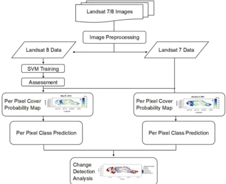
4.2 Materials and Methods ... 78
4.2.1 Satellite Data Used ... 78
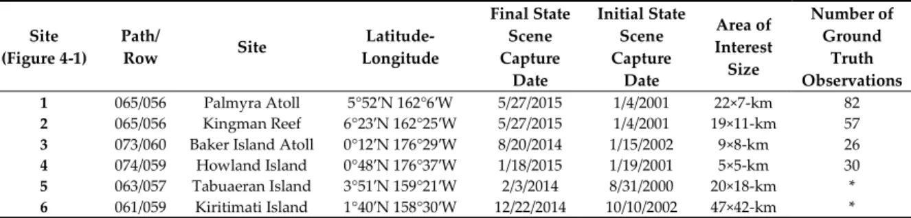
4.2.2 Ground Truth Data Used for Training and Validation... 80
4.2.3 Sites ... 82
4.3 Methodology ... 84
4.3.1 Cloud Mask ... 86
4.3.2 Land Mask ... 87
4.3.3 Atmospheric Correction and Water Column Correction ... 87
4.3.4 SVM Site Application, Validation, and Change Analysis ... 88
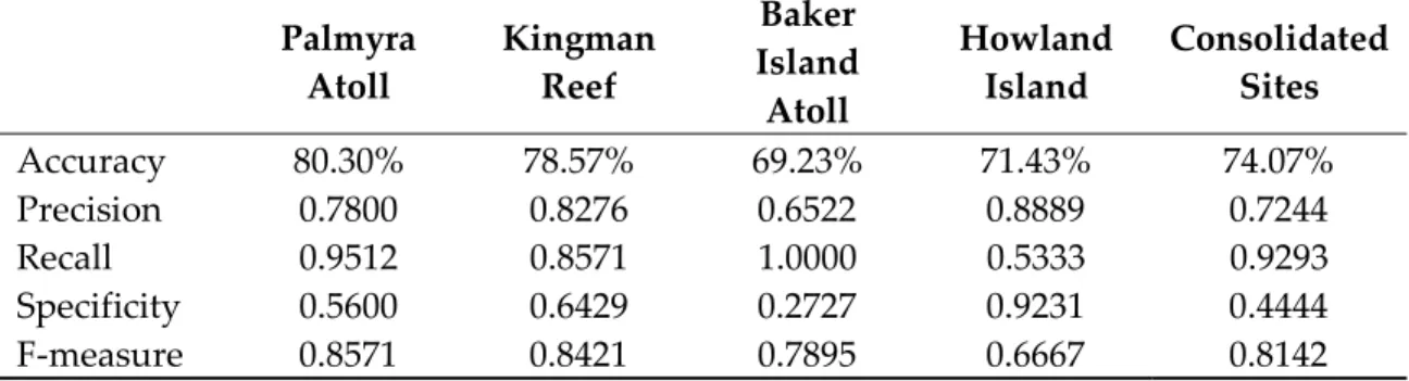
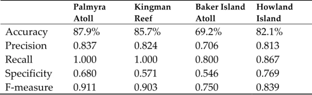
4.4 Results ... 91
4.4.1 Classification Accuracy by Site ... 91
4.4.2 Consolidated Model Robust to Site-Specific Bias ... 94
4.5 Change Detection Analysis ... 97
4.5.1 Palmyra Atoll ... 97
4.5.2 Kingman Reef ... 100
4.5.3 Baker Island Atoll ... 103
4.5.4 Howland Island ... 106
4.5.5 Tabuaeran Island ... 109
4.5.6 Kiritimati Island ... 112
4.6 Discussion ... 116
5. THIRD STUDY: A GENERALIZED MACHINE LEARNING CLASSIFIER FOR SPATIOTEMPORAL ANALYSIS OF CORAL REEFS IN THE RED SEA
... 121
5.1 Introduction ... 121
5.2 Materials and Methods ... 123
5.2.1 Study Area ... 123
5.2.2 Data Used and Preprocessing Steps ... 124
5.2.3 Preprocessing ... 125
5.2.4 Generalized Machine Learning Classifier ... 126
5.3 Results ... 130
5.3.1 Classification Accuracy by Site ... 130
5.3.2 Consolidated Model Robust to Site-Specific Bias ... 133
5.3.3 Change Detection Analysis ... 135
5.4 Discussion ... 145
5.5 Conclusion ... 147
6. CONCLUSION ... 149
LIST OF TABLES
Page
Table 1-1: SDG 13 Targets and Indicators ... 5
Table 1-2: SDG 14 Targets and Indicators ... 8
Table 2-1: Selected Scenes for Study ... 18
Table 3-1: Selected Scenes for Study ... 45
Table 3-2: Selected Scenes for Study, Additional Information ... 46
Table 3-3: Assessment Metrics for Evaluation of Model Performance for Each Site and Consolidated Input. ... 66
Table 3-4: Confusion Matrices by Site and Consolidated Inputs. ... 66
Table 4-1: Image Capture Date and Ground Truth Observation Period for each Location. ... 79
Table 4-2: Satellite Data Summary. ... 80
Table 4-3: SVM Classifier Performance Assessment by Site. ... 93
Table 4-4: Confusion Matrices by Site and Consolidated Inputs. ... 93
Table 4-5: Controlled Parameter Cross-Validation (CPCV) procedure results by site. ... 96
Table 4-6: Change Detection Analysis by Site. ... 115
Table 4-7: Classification accuracy of select additional learning algorithms. ... 117
Table 5-1: Summary of Data Used. ... 125
Table 5-2: SVM Classifier Performance Assessment by Site and Consolidated Model. 132 Table 5-3: Confusion Matrix by Site and the Consolidated Model. ... 133
LIST OF FIGURES
Page
Figure 1-1: World Economic Forum Global Risks Landscape. ... 13 Figure 2-1: Scene masking, atmospheric correction, and water column correction process flow. ... 20 Figure 2-2: Top: Comparison of mean deep-water radiance for Landsat 8 band 2, band 3, and band 4 for each of the 29 scenes selected for analysis. Bottom: Comparison of standard deviation of deep-water radiance. ... 26 Figure 2-3: Comparison of variance in radiance for each band. Certain scenes show more variance due to unique geographic characteristics. ... 29 Figure 2-4: Comparison of covariance of spectral radiance between bands. ... 29 Figure 2-5: Comparison of the atmospheric and surface reflection correction constant (a) for each scene and pair of bands. ... 29 Figure 2-6: Comparison of ration of attenuation for scene and pair of bands. ... 30 Figure 2-7: Left to right: water masked scene, band 2/3 depth invariant index, band 2/4 depth invariant index, band 3/4 depth invariant index. Top to bottom: 013-055 Panama Coiba National Park, 013-057 Colombia Malpelo Fauna and Flora Sanctuary, 015-043 USA Everglades National Park, 016-053 Costa Rica Area de Conservación Guanacaste, 016-056 Costa Rica Cocos Island National Park. ... 33 Figure 2-8: Left to right: water masked scene, band 2/3 depth invariant index, band 2/4 depth invariant index, band 3/4 depth invariant index. Top to bottom: 018-047 Mexico Sian Ka’an, 018-048 Belize Belize Barrier Reef Reserve System, 018-060 Ecuador Galápagos Islands, 034-047 Mexico Archipiélago de Revillagigedo, 038-039 Mexico Sea of Cortez... 34 Figure 2-9: Left to right: water masked scene, band 2/3 depth invariant index, band 2/4 depth invariant index, band 3/4 depth invariant index. Top to bottom: 069-063 Kiribati Phoenix Islands Protected Area, 073-042 USA Papahãnaumokuãkea, 083-074 France Lagoons of New Caledonia, 085-082 Australia Lord Howe Islands, 087-069 Solomon Islands East Rennell. ... 35 Figure 2-10: Left to right: water masked scene, band 2/3 depth invariant index, band 2/4 depth invariant index, band 3/4 depth invariant index. Top to bottom: 091-075 Australia Great Barrier Reef, 104-041 Japan Ogasawara Islands, 106-055 Palau Rock Islands Southern Lagoon, 114-066 Indonesia Komodo National Park, 114-080 Australia
Figure 2-11: Left to right: water masked scene, band 2/3 depth invariant index, band 2/4 depth invariant index, band 3/4 depth invariant index. Top to bottom: 115-078 Australia Shark Bay, Western Australia, 116-054 Philippines Tubbataha Reefs Natural Park, 123-065 Indonesia Ujung Kulon National Park, 126-046 Viet Nam Gulf of Tonkin, 159-051 Yemen Socotra Archipelago. ... 37 Figure 2-12: Left to right: water masked scene, band 2/3 depth invariant index, band 2/4 depth invariant index, band 3/4 depth invariant index. Top to bottom: 161-067 Seychelles Aldabra Atoll, 167-079 South Africa Simangaliso Wetland Park, 170-047 Sudan
Sanganeb Marine National Park, 213-063 Brazil Brazilian Atlantic. ... 38 Figure 3-1 The location of the four sites (1) Palmyra Atoll (2) Kingman Reef (3) Baker Island Atoll (4) Howland Island ... 46 Figure 3-2 Scene masking, atmospheric correction, and water column correction process flow. ... 51 Figure 3-3: Palmyra Atoll: Plot of the posterior probability for belonging to the coral class for each pixel in the Palmyra Atoll site. ... 55 Figure 3-4: Palmyra Atoll predicted class membership based on posterior probabilities. 55 Figure 3-5: Kingman Reef: Plot of the posterior probability for belonging to the coral class for each pixel in the Kingman Reef site. ... 57 Figure 3-6: Kingman Reef predicted class membership based on posterior probabilities. ... 57 Figure 3-7: Baker Island Atoll: Plot of the posterior probability for belonging to the coral class for each pixel in the Baker Island Atoll site. ... 60 Figure 3-8: Baker Island Atoll predicted class membership based on posterior
probabilities... 61 Figure 3-9: Howland Island: Plot of the posterior probability for belonging to the coral class for each pixel in the Howland Island site. ... 63 Figure 3-10: Howland Island predicted class membership based on posterior
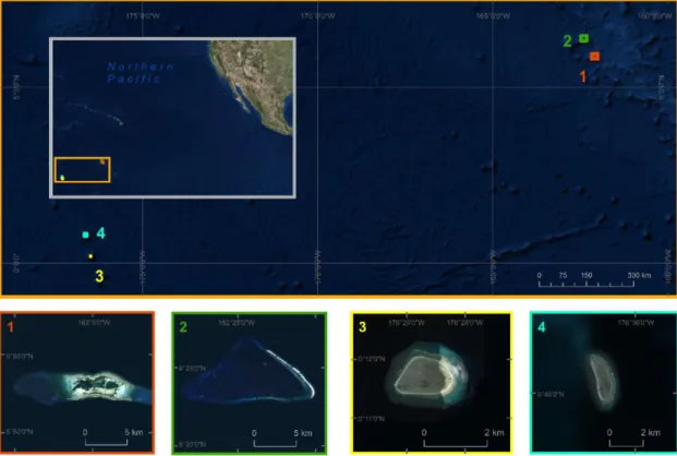
probabilities... 64 Figure 3-11: ROC Curve indicating model performance of the algorithm when applied to the consolidated ground truth set (AUC = 0.7298) ... 69 Figure 4-1: The relative location of each of the six sites (1) Palmyra Atoll, (2) Kingman Reef, (3) Baker Island Atoll, (4) Howland Island, (5) Tabuaeran Island, and (6) Kiritimati Island. ... 84
Figure 4-2: SVM classifier training and change analysis process flow for Palmyra Atoll, Kingman Reef, Baker Island Atoll, and Howland Island. ... 85 Figure 4-3: Robust SVM Classifier training and change analysis process flow for
Tabuaeran Island and Kiritimati Island... 86 Figure 4-4: Performance evaluation of the combined classifier using ROC Curve and AUC (0.778). ... 96 Figure 4-5: Posterior probability map for the Palmyra Atoll area of interest (top, 2001 and bottom, 2015). ... 98 Figure 4-6: Predicted class map for the Palmyra Atoll area of interest (top, 2001 and bottom, 2015). ... 99 Figure 4-7: Difference in predicted class membership map for the Palmyra Atoll area of interest for 2001 initial state compared to 2015 final state. ... 99 Figure 4-8: Posterior probability map for the Kingman Reef area of interest (top, 2001 and bottom, 2015). ... 101 Figure 4-9: Predicted class probability map for the Kingman Reef area of interest (top, 2001 and bottom, 2015). ... 102 Figure 4-10: Difference in predicted class membership map for the Kingman Reef area of interest for 2001 initial state compared to 2015 final state. ... 103 Figure 4-11: Posterior probability map for the Baker Island Atoll area of interest (top, 2002 and bottom, 2014). ... 104 Figure 4-12: Predicted class map for the Baker Island Atoll area of interest (top, 2002 and bottom, 2014). ... 105 Figure 4-13: Difference in predicted class membership map for the Palmyra Atoll area of interest for 2002 initial state compared to 2014 final state. ... 106 Figure 4-14: Posterior probability map for the Howland Island area of interest (top, 2001 and bottom, 2015). ... 107 Figure 4-15: Predicted class map for the Howland Island area of interest (top, 2001 and bottom, 2015). ... 108 Figure 4-16: Difference in predicted class membership map for the Howland Island area of interest for 2001 initial state compared to 2015 final state... 109 Figure 4-17: Posterior probability map for the Tabuaeran Island area of interest (top, 2000 and bottom, 2014). ... 110
Figure 4-18: Predicted class map for the Tabuaeran Island area of interest (top, 2000 and bottom, 2014). ... 111 Figure 4-19: Difference in predicted class membership map for the Tabuaeran Island area of interest for 2000 initial state compared to 2014 final state... 112 Figure 4-20: Posterior probability map for the Kiritimati Island area of interest (top, 2002 and bottom, 2014). ... 113 Figure 4-21: Predicted class map for the Kiritimati Island area of interest (top, 2002 and bottom, 2014). ... 114 Figure 4-22: Difference in predicted class membership map for the Kiritimati Island area of interest for 2002 initial state compared to 2014 final state... 115 Figure 5-1: Relative location of the three locations under study (1) Gulf of Aqaba
Location, (2) Umluj Location, (3) Al Wajh Location ... 124 Figure 5-2: SVM Classifier training (Gulf of Aqaba), validation (Umluj), and application of the robust classifier (Al Wajh)... 129 Figure 5-3: Temporal change detection analysis process flow. ... 130 Figure 5-4: Performance evaluation of the robust, combined classifier using ROC Curve and AUC for the Gulf of Aqaba and consolidated model. ... 135 Figure 5-5: Posterior probability map for the Gulf of Aqaba area of interest (top, 2000 and bottom, 2018). ... 137 Figure 5-6: Predicted class membership map for the Gulf of Aqaba area of interest (top, 2000 and bottom, 2018). ... 138 Figure 5-7: Change detection analysis between 2000 and 2018 of the Gulf of Aqaba area of interest. ... 139 Figure 5-8: Posterior probability map for the Umluj area of interest (left, 2000 and right, 2018). ... 140 Figure 5-9: Predicted class membership map for the Umluj area of interest (left, 2000 and right, 2018). ... 141 Figure 5-10: Change detection analysis between 2000 and 2018 of the Umluj area of interest. ... 142 Figure 5-11: Posterior probability map for the Al Wajh area of interest (left, 2000 and right, 2018). ... 143
Figure 5-13: Change detection analysis between 2000 and 2018 of the Al Wajh area of interest. ... 144
1.
Introduction
1.1
Goals of this Research
Previous research concerning the analysis of coral reefs using remote sensing data has been limited to in-situ analysis. That is, these studies have isolated specific reefs or a small area of interest (AOI) in order to perform benthic habitat cover detection using remote sensing data. These studies achieve a remarkable level of accuracy particularly if based on high resolution imagery. Often, these analyses can achieve upwards of 90% class prediction accuracy when compared to ground truth observation data [1]. The recent abundance of high-resolution satellite platforms enables these scientific studies and their results are quite promising with respect to analyzing the individual reefs they target for the time period in which remote sensing data from their platform of choice is available. However, there are two challenges faced by these studies. First, they rely upon high resolution remote sensing data and second, they are spatially limited in scope.
Recent advances in technology have enabled high-resolution remote sensing imagery. While these satellites enable benthic habitat classification with a high degree of accuracy, they do not enable the historical archive necessary for long-term temporal change detection analysis. The Landsat missions, on the other hand, afford a rich archive of historical imagery. This data enables long-term change analysis, defined here as greater than 10-years. Yet, the Landsat platform is limited to medium resolution data both now
and historically. Even though the technology for much higher resolution sensors is available, Landsat has maintained a 30m x 30m pixel resolution. This was intentionally done in order to maintain parity with previous missions. As a result, the Landsat platform is the most common source of remote sensing data for change detection analysis of coral reefs as well as all other benthic and land cover types [1].
Secondly, previous research has been limited in scope spatially. An abundance of scientific studies are available which have isolated a specific reef or small AOI within which benthic cover type detection or change detection analysis is performed. These in-situ analyses are, by definition, limited in scope. Studies conducted in this way often yield accuracies, measured by the percentage of pixel cover types matching ground truth observations, of 85% or greater. Yet, the isolation of a specific area for both training and analysis necessarily mean that these analyses are often overfit to that specific location. That is, the classifiers used to evaluate the reef are both trained and tested using data from the same location. As a result, these classifiers will not perform well if applied to a new location. This is because the training and testing methodology employed to create the models causes them to be significantly overfit to the local conditions represented in the respective AOI. In this way, in-situ analyses rely upon site-specific biases that prevent them from generalizing to new locations. These classifiers memorize the site-specific geomorphology, fauna, and other local conditions at the specific site. Therefore, while the classifiers serve the purpose as it pertains to the specific location under analysis, they will not generalize to new locations.
The goal of this research is to develop a robust machine learning classifier that can generalize spatially beyond the scope of previous in-situ type analyses. The proposed methodology includes using remote sensing data from multiple sites and the associated ground truth data in order to develop a robust classifier that can generalize beyond any single AOI. In order to measure the effectiveness of the generalized classifier, the Controlled Parameter Cross-Validation (CPCV) evaluation procedure is proposed. This methodology accounts for site-specific information that may bias the results of standard train/test split or cross-validation methods and provides a more accurate assessment of how well the classifier is generalizing to new data.
1.2
2030 Agenda for Sustainable Development
The 2030 Agenda for Sustainable Development was adopted by all United Nations (UN) Member States in 2015. This agenda seeks to build on the Millennium Development Goals and complete what they did not achieve. The agenda includes 17 Sustainable Development Goals (SDGs), 169 targets, and 232 indicators all aimed at establishing principles of sustainable development in national policies. The research proposed in this dissertation addresses two of these goals. In particular, SDG 13 concerning climate action and SDG 14 concerning life below water.
The objective of SDG 13 is to take urgent action to combat climate change and its impacts. To achieve this, SDG 13 asserts five different targets. Table 1-1 shows each of these targets and the associated indicator(s). Goal 13.3 asserts, “Improve education, awareness-raising and human and institutional capacity on climate change mitigation,
performs two functions to contribute to this goal. First, it informs countries on mitigation, adaptation, and impact reduction data from which curricula can be based. This contributes to the first indicator, “Number of countries that have integrated mitigation, adaptation, impact reduction and early warning into primary, secondary and tertiary curricula.” Curricula must be based on scientific study and results. This research provides a methodology for developing results with respect to coral reef extent as well as evaluation of results from the proposed methodology. The research proposed in this dissertation addresses the second indicator, “Number of countries that have communicated the strengthening of institutional, systemic and individual capacity-building to implement adaptation, mitigation and technology transfer, and development actions.” By informing countries, particularly those with significant coastal habitats, of their exposure to climate change this research enables those countries to more effectively strengthen capacity-building to implement adaption and mitigation actions. In addition, this research contributes to the indicators behind target 13.B, “Promote mechanisms for raising capacity for effective climate change-related planning and management in least developed countries and small island developing States, including focusing on women, youth and local and marginalized communities” by informing small developing island states such as Kiribati of their exposure to climate-change. Kiribati is a small island country with significant populations on Kiritimati Island and Tabuaeran Island both of which are included in this research. Informing this small island developing State of their exposure to climate-change risk addressed the associate SDG indicator, “Number of least developed countries and small island developing States that are receiving specialized support, and amount of support, including finance, technology and capacity-building, for mechanisms for raising
capacities for effective climate change-related planning and management, including focusing on women, youth and local and marginalized communities” by directly informing at least one such island country. In addition to these direct implications of this research there are several indirect impacts. For example, this research can be used to inform target 13.2, “Integrate climate change measures into national policies, strategies and planning” by informing policy makers of the specific, localized impact associated with their directives.
Table 1-1: SDG 13 Targets and Indicators
Targets Indicators
13.1 Strengthen resilience and adaptive capacity to climate-related hazards and natural disasters in all countries
13.1.1 Number of deaths, missing persons and persons affected by disaster per 100,000 people
13.1.2 Number of countries with national and local disaster risk reduction strategies 13.1.3 Proportion of local governments that adopt and implement local disaster risk reduction strategies in line with national disaster risk reduction strategies 13.2 Integrate climate change measures
into national policies, strategies and planning
13.2.1 Number of countries that have communicated the establishment or operationalization of an integrated
policy/strategy/plan which increases their ability to adapt to the adverse impacts of climate change, and foster climate resilience and low greenhouse gas emissions development in a manner that does not threaten food production (including a national adaptation plan, nationally determined contribution, national communication, biennial update report or other)
Table 1-1 (cont.): SDG 13 Targets and Indicators
Targets Indicators
13.3 Improve education, awareness-raising and human and institutional capacity on climate change mitigation, adaptation, impact reduction and early warning
13.3.1 Number of countries that have integrated mitigation, adaptation, impact reduction and early warning into primary, secondary and tertiary curricula
13.3.2 Number of countries that have communicated the strengthening of institutional, systemic and individual capacity-building to implement adaptation, mitigation and technology transfer, and development actions 13.A Implement the commitment
undertaken by developed-country parties to the United Nations Framework
Convention on Climate Change to a goal of mobilizing jointly $100 billion
annually by 2020 from all sources to address the needs of developing countries in the context of meaningful mitigation actions and transparency on
implementation and fully operationalize the Green Climate Fund through its capitalization as soon as possible
13.A.1 Mobilized amount of United States dollars per year starting in 2020
accountable towards the $100 billion commitment
13.B Promote mechanisms for raising capacity for effective climate change-related planning and management in least developed countries and small island developing States, including focusing on women, youth and local and marginalized communities
13.B.1 Number of least developed countries and small island developing States that are receiving specialized support, and amount of support, including finance, technology and capacity-building, for mechanisms for raising capacities for effective climate change-related planning and management, including focusing on women, youth and local and marginalized communities
SDG 14 aims to conserve and sustainably use the oceans, seas, and marine resources for sustainable development. Table 1-2 shows each of the targets of SDG 14 and the associated indicator(s). Of the 10 SDG targets set to achieve this goal, at least three are directly related to the research presented in this dissertation. First, target 14.2 states, “By 2020, sustainably manage and protect marine and coastal ecosystems to avoid significant
adverse impacts, including by strengthening their resilience, and take action for their restoration in order to achieve healthy and productive oceans.” This target is enabled by identifying coastal ecosystems most susceptible to adverse impacts thereby enabling local governments to take action and protect their valuable coastal resources. The indicator associated with this target is 14.2.1, “Proportion of national exclusive economic zones managed using ecosystem-based approaches” which can only be enabled by identifying the ecosystems impacted by said approaches. Furthermore, target 14.5 calls for, “By 2020, conserve at least 10 per cent of coastal and marine areas, consistent with national and international law and based on the best available scientific information.” The scientific information delivered in these studies directly impacts this target and informs the associated indicator, “Coverage of protected areas in relation to marine areas,” by identifying the extent of one of the key marine areas that is called to be protected. Finally, target 14.A indicates, “Increase scientific knowledge, develop research capacity and transfer marine technology, taking into account the Intergovernmental Oceanographic Commission Criteria and Guidelines on the Transfer of Marine Technology, in order to improve ocean health and to enhance the contribution of marine biodiversity to the development of developing countries, in particular small island developing States and least developed countries.” The methodology proposed in this research directly contributes to this target through increasing scientific knowledge and developing research capacity which improves ocean health and marine biodiversity to Kiribati and similar small island developing States. In addition to these direct influences, the research presented in this dissertation address multiple targets and indicators associated with SDG 14 indirectly.
These indirect implications as well as the direct consequences of this research aggregate to a significant total influence that is ambitions with far-reaching impact.
Table 1-2: SDG 14 Targets and Indicators
Targets Indicators
14.1 By 2025, prevent and significantly reduce marine pollution of all kinds, in particular from land-based activities, including marine debris and nutrient pollution
14.1.1 Index of coastal eutrophication and floating plastic debris density
14.2 By 2020, sustainably manage and protect marine and coastal ecosystems to avoid significant adverse impacts, including by strengthening their resilience, and take action for their
restoration in order to achieve healthy and productive oceans
14.2.1 Proportion of national exclusive economic zones managed using
ecosystem-based approaches
14.3 Minimize and address the impacts of ocean acidification, including through enhanced scientific cooperation at all levels
14.3.1 Average marine acidity (pH) measured at agreed suite of representative sampling stations
14.4 By 2020, effectively regulate harvesting and end overfishing, illegal, unreported and unregulated fishing and destructive fishing practices and
implement science-based management plans, in order to restore fish stocks in the shortest time feasible, at least to levels that can produce maximum sustainable yield as determined by their biological characteristics
14.4.1 Proportion of fish stocks within biologically sustainable levels
14.5 By 2020, conserve at least 10 per cent of coastal and marine areas,
consistent with national and international law and based on the best available scientific information
14.5.1 Coverage of protected areas in relation to marine areas
Table 2-2 (cont.): SDG 14 Targets and Indicators
Targets Indicators
14.6 By 2020, prohibit certain forms of fisheries subsidies which contribute to overcapacity and overfishing, eliminate subsidies that contribute to illegal, unreported and unregulated fishing and refrain from introducing new such subsidies, recognizing that appropriate and effective special and differential treatment for developing and least
developed countries should be an integral part of the World Trade Organization fisheries subsidies negotiation
14.6.1 By 2020, prohibit certain forms of fisheries subsidies which contribute to overcapacity and overfishing, eliminate subsidies that contribute to illegal, unreported and unregulated fishing and refrain from introducing new such subsidies, recognizing that appropriate and effective special and differential treatment for developing and least
developed countries should be an integral part of the World Trade Organization fisheries subsidies negotiation
14.7 By 2030, increase the economic benefits to Small Island developing States and least developed countries from the sustainable use of marine resources, including through sustainable
management of fisheries, aquaculture and tourism
14.7.1 Sustainable fisheries as a percentage of GDP in small island developing States, least developed countries and all countries
14.A Increase scientific knowledge, develop research capacity and transfer marine technology, taking into account the Intergovernmental Oceanographic Commission Criteria and Guidelines on the Transfer of Marine Technology, in order to improve ocean health and to enhance the contribution of marine biodiversity to the development of developing countries, in particular small island developing States and least developed countries
14.A.1 Proportion of total research budget allocated to research in the field of marine technology
14.B Provide access for small-scale artisanal fishers to marine resources and markets
14.B.1 Progress by countries in the degree of application of a
legal/regulatory/policy/institutional framework which recognizes and protects access rights for small-scale fisheries
Table 2-2 (cont.): SDG 14 Targets and Indicators
Targets Indicators
14.C Enhance the conservation and sustainable use of oceans and their resources by implementing international law as reflected in UNCLOS, which provides the legal framework for the conservation and sustainable use of oceans and their resources, as recalled in paragraph 158 of The Future We Want
14.C.1 Number of countries making progress in ratifying, accepting and implementing through legal, policy and institutional frameworks, ocean-related instruments that implement international law, as reflected in the United Nation Convention on the Law of the Sea, for the conservation and sustainable use of the oceans and their resources
1.3
Paris Agreement
The Paris Agreement was signed on April 22, 2016. The goal of this doctrine is to keep the increase in global average temperature to well below 2°C. Associated with this agreement are several articles stipulated in order to achieve the goal. First Article 8 states, “Parties recognize the importance of averting, minimizing and addressing loss and damage associated with the adverse effects of climate change, including extreme weather events and slow onset events, and the role of sustainable development in reducing the risk of loss and damage.” The deterioration of coral reefs as a result of temperature increases is a significant impact related to slow onset events. The research presented in this dissertation addresses this aspect of the article by informing the loss and damage to coral reefs related to temperature change. Second article 12 asserts, “Climate change education, training, public awareness, public participation and public access to information (Art 12) is also to be enhanced under the Agreement” and core to this is information regarding the impact of climate-change on coral reefs. Definitively measuring this impact significantly enhances the public awareness, public participation, and public access as it enables both the availability of data and the visibility into who and what is being impacted. The research
Finally, Article 14 of the Paris Agreement decrees, “A global stocktake, to take place in 2023 and every 5 years thereafter, will assess collective progress toward meeting the purpose of the Agreement in a comprehensive and facilitative manner. Its outcomes will inform Parties in updating and enhancing their actions and support and enhancing international cooperation.” This is directly supported by the research proposed in this dissertation which performs a significant stock-take of Pacific Ocean and Red Sea coral as well as enables a global stock-take of coral reefs.
1.4
Sendai Framework for Disaster Risk Reduction
The Sendai Framework for Disaster Risk Reduction aims for: “The substantial reduction of disaster risk and losses in lives, livelihoods and health and in the economic, physical, social, cultural and environmental assets of persons, businesses, communities and countries.” To this end, the research presented in this dissertation addresses the environmental assets of persons, businesses, communities, and countries. Specifically, the primary resource of many countries is their marine environment and, in particular, the costal reefs marine environment. This ecosystem provides many communities with a local resource for income (tourism or otherwise) and sustenance (through fishing, research, or otherwise). Therefore, the health of this local resource is critical to the lives, livelihoods, and health of local communities economically, physically, socially, culturally, and environmentally. Particularly with respect to the Kiritimati Island and Tabuaeran Island communities as well as the small Red Sea villages which rely on the coral reefs for subsistence, the results of this research are imperative to inform policy and decision making.
1.5
World Economic Forum: The Global Risks Report
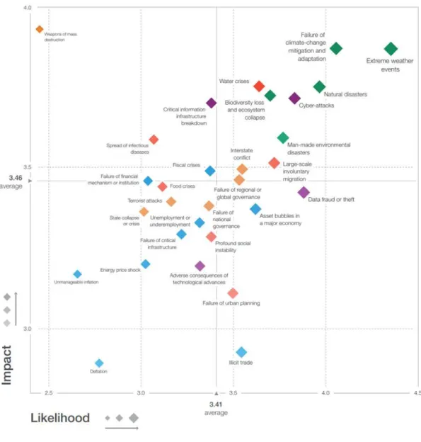
The Global Risks Report is an annual evaluation by the World Economic Forum which looks at the foremost risks facing the world [2]. These risks range from weapons of mass destruction to terrorist attacks to financial crisis. There are several methods by which the World Economic Forum reports on these risks. One such methodology is a visualization called the Global Risks Landscape. This visualization plots each primary global risk on a scale by likelihood on the x-axis and impact on the y-axis. Therefore, global risks that are higher on the plot represent a larger impact while global risks that are to the right of the plot represent a larger likelihood. In 2019, all environmental risks were represented in the first quadrant as both most likely and most impactful, Figure 1-1.
Figure 1-1: World Economic Forum Global Risks Landscape.
Furthermore, failure of climate-change mitigation and adaptation was both the second most likely risk and second highest impact risk. This risk represents the failure of governments and businesses to recognize and react to climate change resulting in catastrophic loss of biodiversity. Since 1970 species abundance is down by 60% and the loss of biodiversity is affecting health and socioeconomic development with implications for productivity and even regional security.
This dissertation directly addresses the failure of climate-change mitigation and adaptation risk outlined in the World Economic Forum Global Risks Report. Specifically, the research proposed identifies the impact that climate-change is having within coral reef ecosystems of both the Red Sea and Pacific Ocean. Coral reefs are the most biodiverse marine ecosystems and among the most biodiverse ecosystems in the world. Therefore, this environment is of utmost important when considering the threat of catastrophic loss of biodiversity. This research is an evaluation of the changing cover across a large extent of coral reef environments and therefore provides valuable information for the governments and businesses addressed in the Global Risks Report. Providing this insight provides data for these organizations to call attention to the need for climate-change mitigation and adaptation. Furthermore, this research is foundational to the global mapping and evaluation of coral reefs. Enabling a robust classifier that can generalize beyond site-specific deployment is the key to understanding and informing climate-change mitigation strategies on a global scale.
2.
Water Column Correction/Depth
Invariant Index
2.1
Introduction
Coral reefs are among the most complex and diverse marine ecosystems in the world [3]. However, these delicate ecosystems are under extreme threat due to numerous environmental and anthropogenic forces. Ocean acidification and mass bleaching events leading to large scale coral death is well documented [4] [5] [6] [7] [8] [9] [10] [11] [12]. Therefore, monitoring of these ecosystems is critical to inform policy and decision making for all agencies and at all levels. A comprehensive plan for evaluating the health of these delicate ecosystems is a complex endeavor that can only be achieved through the combined efforts of both detailed in-situ analyses and efficient, large scale analyses. Traditionally, reefs have been monitored using expensive and tedious underwater surveying techniques [13] [14] [15] [16] [17] [18] [19] [20] that, by definition, cannot cover large areas [21]. These traditional techniques have several drawbacks that restrict their use and the relevance of outcomes. These are (1) cost-related: detailed, continuous monitoring of coral reefs by field survey is expensive and substantial reef areas are located in developing countries with limited resources; (2) scale-related: reefs are highly heterogeneous systems [22] [23], therefore, even with sufficient resources, monitoring programs provide scattered
and less easily accessible areas being under-sampled; and (3) focus-related: most field monitoring programs are focused on the state variables describing some of the biological components of the reef system and are not linked explicitly to the identification of stressors or processes [4]. As such, satellite observations serve as a useful mean of timely and cost effective global monitoring and surveying of large and remote coral reef areas globally that could otherwise not be achieved [24] [25] [26]. The most common sensors suitable for subsurface, ocean floor cover identification are SPOT High-Resolution Visible (HRV), Landsat Multispectral Scanner (MSS), Thematic Mapper (TM), Enhanced Thematic Mapper Plus (ETM+), Operational Land Imager (OLI), IKONOS, Advanced Airborne Hyperspectral Imaging System (AAHIS), Airborne Visible/Infrared Imaging Spectrometer (AVIRIS), and Sentinel-2 [4] [27] [28] [29] [30] [31] [32] [33] [34]. In addition, it is noteworthy that there are many more satellites available that are capable of providing remote sensing data for coral reef analysis [25] [26] [35]. Visible spectrum is known to be useful in mapping of subsurface habitats [36] [37] [38]. This is owed to the fact that wavelengths (400nm-600nm) have ~15-3m penetration through clear waters, depending on turbidity and water quality [39]. However, this penetration depth is wavelength dependent as it increases with longer wavelengths [40]. As a result, the blue spectral bands (400nm) attenuate more slowly than red spectral bands (600nm) [1]. Moreover, underwater marine environment detection doesn’t only come with spatial and spectral limitations challenges, but also the confounding influence variable depth on bottom reflectance, and disturbances due to turbidity of the water column [41] [42] [43] [44]. These factors significantly influence the spectral reflectance of the seafloor, thereby causing identical bottom types to exhibit substantially different characteristics in remote sensing data [45] [46]. Therefore,
water column and atmospheric corrections are needed in order to accurately detect the existence of coral within a pixel [47] [48] [49].
In this study, we considered 29 different scenes with known benthic regions. We implemented a process which accounts for any interferences in the image (clouds, dropped pixels, etc), applied a water mask, corrected for atmospheric obstructions, then calculated each of the depth invariant indices across the image. To better understand the output, we plotted each of the depth invariant indices as an image and observed the differences between the plots. This analysis showed that depth invariant index can be applied to a variety of ocean scenes throughout the world, with limited variance in the resulting output parameters. Furthermore, the results from this analysis can be used as inputs to a classification algorithm in order to rapidly identify benthic zone cover types, enabling large-scale, multi-temporal change detection.
2.2
Data Used
Images from Landsat-8 OLI with 30m spatial resolution were used to conduct the survey. The visible bands were used due to their water column penetration properties with band 1 corresponding to 0.433-0.453µm, band 2 corresponding to 0.450-0.515µm, band 3 corresponding to 0.525-0.600µm, and band 4 corresponding to 0.630-0.680µm. It is noteworthy that the previous visible bands have the spectral range that can help in identifying water-land interface. In addition, band 5, which represents near infrared (NIR), was used to identify areas of full wavelength absorption for water masking. Scenes were selected based on the existence of corals in benthic zones. Landsat 8 images were first
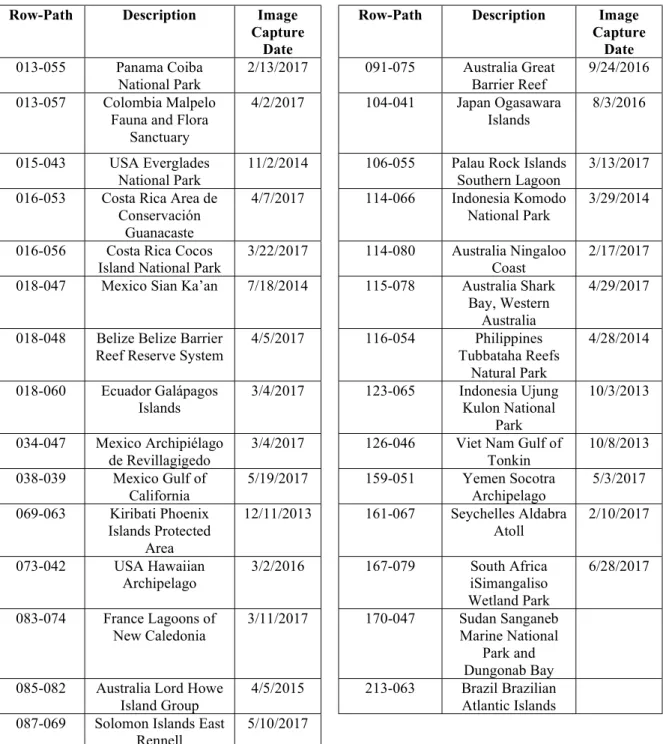
images were then visually inspected to determine which were most appropriate, including factoring in the location of clouds and other disturbances in the locations of known corals. In total 29 different scenes were selected. A listing of each site and the associated Landsat scene Row-Path reference is provided in Table 2-1:
Table 2-1: Selected Scenes for Study
Row-Path Description Image Capture
Date
Row-Path Description Image Capture
Date
013-055 Panama Coiba
National Park 2/13/2017 091-075 Australia Great Barrier Reef 9/24/2016 013-057 Colombia Malpelo
Fauna and Flora Sanctuary
4/2/2017 104-041 Japan Ogasawara
Islands 8/3/2016 015-043 USA Everglades
National Park 11/2/2014 106-055 Palau Rock Islands Southern Lagoon 3/13/2017 016-053 Costa Rica Area de
Conservación Guanacaste
4/7/2017 114-066 Indonesia Komodo
National Park 3/29/2014 016-056 Costa Rica Cocos
Island National Park 3/22/2017 114-080 Australia Ningaloo Coast 2/17/2017 018-047 Mexico Sian Ka’an 7/18/2014 115-078 Australia Shark
Bay, Western Australia
4/29/2017 018-048 Belize Belize Barrier
Reef Reserve System 4/5/2017 116-054 Tubbataha Reefs Philippines Natural Park
4/28/2014 018-060 Ecuador Galápagos
Islands 3/4/2017 123-065 Indonesia Ujung Kulon National Park
10/3/2013 034-047 Mexico Archipiélago
de Revillagigedo 3/4/2017 126-046 Viet Nam Gulf of Tonkin 10/8/2013 038-039 Mexico Gulf of California 5/19/2017 159-051 Yemen Socotra Archipelago 5/3/2017 069-063 Kiribati Phoenix Islands Protected Area 12/11/2013 161-067 Seychelles Aldabra Atoll 2/10/2017 073-042 USA Hawaiian
Archipelago 3/2/2016 167-079 iSimangaliso South Africa Wetland Park 6/28/2017 083-074 France Lagoons of New Caledonia 3/11/2017 170-047 Sudan Sanganeb Marine National Park and Dungonab Bay 085-082 Australia Lord Howe
Island Group
4/5/2015 213-063 Brazil Brazilian Atlantic Islands 087-069 Solomon Islands East
2.3
Methodology
The overall layout of the processing approach applied to the 29 selected scenes is shown in Figure 2-1. This approach can be broken down into three major components: preprocessing the image (cloud, quality, and land/water masking), atmospheric correction, and water column correction. Scenes were selected to minimize the presence of clouds in the image. Pixels that still suffer cloud cover or other obstructions were then identified by leveraging the Landsat BQA band and masked accordingly. This is followed by creating a water mask by applying a threshold to the NIR band. This is carried out because the water body and corals have similar spectral reflectance, which may lead to misclassification in water/coral areas. A deep-water AOI was selected to be used in atmospheric correction via the dark-pixel subtraction method [37] [50] [51]. These adjustments were applied to each of the visible bands before the depth invariant indices were calculated. Analysis was conducted using the open source R programming language and environment for statistical computing [52].
Figure 2-1: Scene masking, atmospheric correction, and water column correction
process flow.
2.3.1
Cloud and Quality Mask
The first step taken in preprocessing the selected images was to identify and mask cloud cover. Great care was taken to select scenes with minimal amount of cloud cover, but in many instances, no available image was completely clear of cloud cover. Masking of clouds was performed by leveraging the Landsat 8 Level 1 product quality band (BQA) [53]. This band includes values for each pixel that, when converted to binary, indicate any potential disturbances with respect to the pixel and a rough approximation of confidence that that condition exists [54]. Converting each observation in this band and thresholding provides a mask to account for some of these conditions. Bits 14 and 15 indicate the likelihood of cloud interference while bits 12 and 13 indicate the possibility of cirrus cloud interference. There are several possible ways in which bias from cloud obstruction can
contaminate an analysis. The obvious entry point is disrupting the reflectance of a pixel or group of pixels. In addition to directly influencing surface reflectance, cloud cover present in the deep-water AOI can alter the values used for atmospheric correction applied to the image through the dark-pixel subtraction method [55]. As a result, this initial step of masking cloud interference is a critical preprocessing step.
2.3.2
Water Mask
The study of DII related metrics across large scenes requires preprocessing that includes masking land as well as clouds. This step is imperative, as including land pixels will severely distort the DII parameters when calculated across the scene. The water mask was created by leveraging the Landsat 8 NIR sensor. This sensor measures light between 0.851 and .0879 micrometers. Water absorbs light in these wavelengths, therefore, it is a good candidate for discerning water from land in any given scene [56]. As in the visible bands, the Landsat 8 NIR band (band 5) is at 30m resolution. A threshold was applied to the NIR band pixel values of each scene. The plots were then evaluated visually to determine the most appropriate cutoff for separation of land and water. A mask was then created for pixels determined to be water.
2.3.3
Atmospheric Correction
In the visual bands, 90% of the at sensor reflectance depends on atmospheric and water surface properties [57]. Therefore, atmospheric correction is first performed using the dark pixel subtraction method [58]. This method selects areas of the scene with water
these areas are comprised of atmospheric radiance and surface reflectance, thereby isolating the impact of these elements. Assuming the atmospheric and water surface conditions generalize to the rest of the scene (i.e. uniform throughout the area of interest), the mean deep-water radiance at sensor can be leveraged to correct for the effect of atmospheric and surface reflectance interferences [1] [59] [60]. Depths greater than 50m will assure that the visible wavelengths have fully attenuated [61]. In addition, two standard deviations are subtracted to account for possible sensor noise [62]. It is important to highlight the assumption that conditions are uniform across each scene. In addition, because of this assumption, the deep-water AOI selected should appear in the same scene that is being analyzed. This will minimize the possibility of unintended bias that may be introduced by leveraging a deep-water AOI of another image and that, to the greatest extent possible, the effect of full attenuation of the wavelengths is isolated. In preprocessing, the deep-water AOI was selected through visual inspection. In some instances, references to external sources were made to verify the appropriate depth.
2.3.4
Water Column Correction
As light penetrates water, the intensity decreases exponentially with increasing depth. The rate of attenuation is wavelength-dependent and has a severe effect on remotely sensed data of aquatic habitats [1]. Therefore, water column correction is appropriate for imagery with multiple water-penetrating spectral bands [51] [63]. Within these visible spectral bands, longer wavelength blue bands attenuate less rapidly than shorter-wavelength red bands. Therefore, the spectral radiances recorded at sensor are dependent on both the subsurface strata reflectance and depth. The confounding influence of depth
can create significant distortions in the subsurface reflectance. Since most marine habitat-mapping exercises are only concerned with habitat-mapping benthic features, it is advantageous to remove the influence of variable depth. The radiance at sensor in band i (𝐿 ) can be expressed as [1] [64] [65] [66]:
𝐿 = 𝐿 + 𝑎 ∙ 𝑟 ∙ 𝑒 (1)
Where the following are represented:
𝐿 : the mean deep-water radiance in band i
𝑎 : a constant for band i accounting for atmospheric effects and water surface reflection
𝑟: the bottom reflectance
𝑓: a geometric factor to account for path length through water (set to two for a two-flow model)
𝑘 : the coefficient of attenuation of band i (to account for various interferences suspended in the water and scattering due to turbidity) [1] [66]
𝑧: depth
Applying natural logarithms and rearranging equation (1) generates an atmospherically corrected radiance for band i that varies linearly according to depth [1]:
Similarly, the equation can be applied to band j:
ln(𝐿 − 𝐿 ) = ln 𝑎 ∙ 𝑟 − 2𝑘 𝑧 (2b)
Equation (2a) can be rearranged to determine the bottom reflectance 𝑟:
ln (𝑟 ) = ( ) (3)
Yet this equation presents us with three unknown variables. Namely, the constant, the coefficient of attenuation, and depth (𝑎, 𝑘 , and 𝑧 respectively). However, by leveraging the ratio of attenuation coefficients between each pair of bands we can avoid calculating estimates of 𝑘 for each band [63] [64]. The ratio of attenuation between bands
i and j can be determined using the following equation:
= 𝑎 + (𝑎 + 1) (4)
where
𝑎 = (5)
and 𝜎 is the variance of band i and 𝜎 is the covariance between bands i and j. Therefore, using these equations, the depth invariant index (DII) can be calculated for any given scene without any external references to additional data.
2.4
Output Parameters
We will now discuss in detail the output and related parameters that result from applying the above methodology to the 29 Landsat 8 scenes.
2.4.1
Image Correction and Deep-Water AOI Parameters
A section of each scene representing deep-water was selected for atmospheric correction using dark-pixel subtraction. The mean deep-water AOI for each scene is shown in Figure 2-2. The highest mean deep-water values for were observed in the Sea of Cortez, Mexico, and the Sudan Sanganeb Marine National Park areas (row-path 038-039 and 170-047, respectively). These two scenes were unique in that they are located in large gulfs. As a result, they are both protected from the influence of currents and associated turbidity. In addition, the deepest water in these scenes is likely shallower than that of other scenes. Finally, both locations are in areas known to be somewhat arid environments with favorable conditions for reducing atmospheric interference.
Figure 2-2: Top: Comparison of mean deep-water radiance for Landsat 8 band 2,
band 3, and band 4 for each of the 29 scenes selected for analysis. Bottom: Comparison of standard deviation of deep-water radiance.
The standard deviation measures were consistent across many of the scenes. The Sea of Cortez, Mexico, showed the largest standard deviation which could also be a product of the location being in a large gulf. In addition, the Phoenix Islands in Kiribati and Ijung Kulon National Park in Indonesia (row-path 123-065) showed higher variance. This could be due to clouds in the selected area. Clouds were masked from the image and an attempt was made to avoid them when selecting the deep-water AOI in each scene.
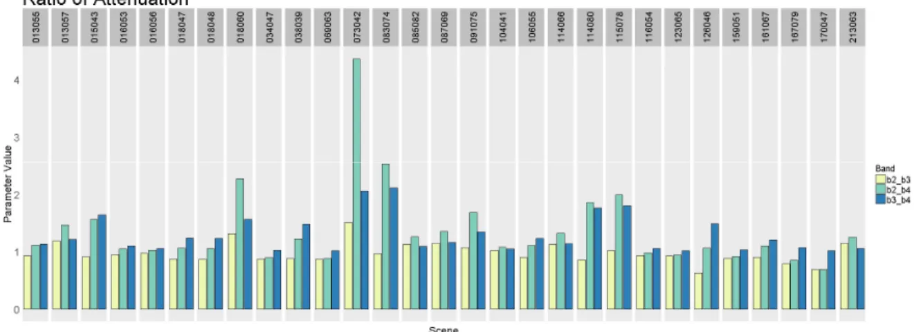
2.4.2
Ratio of Attenuation
The ratio of attenuation is calculated from variance and covariance of the bands. The variance and covariance were calculated based on the atmospherically corrected and masked water pixels only. Figure 2-3 and figure 2-4 display the resulting variance and covariance for each scene. Several scenes stand out as having very high variance in radiance. This is due to unique geographical characteristics of those regions. The Everglades National Park in Florida, USA, (row-path 015-043) is known for its expansive wetlands. This unique aquatic environment contains very shallow waters mixed with a high concentration of vegetation. Regions such as this will absorb wavelengths in the NIR spectrum and therefore are appropriately classified as water. Furthermore, by the very nature of the environment, its spectral radiance exhibits a high degree of variance as an abundance of very shallow cover is detected within the image. Similarly, Australia’s Shark Bay exhibits a high degree of variance likely due to the spectral radiance and ecology of very shallow waters.
The covariance of band radiation reveals similar characteristics to the variance of the bands. That is, scenes with regions dominated by shallow waters such as the Everglades National Park in Florida, USA, and Shark Bay, Australia, have a high degree of variance in spectral radiance between the bands. This is an expected result as a larger variety of vegetation has evolved to live in these aquatic environments.
With the variance and covariance known, we can calculate the constant used to account for atmospheric effects and water surface reflection (a) for each scene. This
by two times the covariance between the bands. The resulting value for the constant (a) for each scene is presented in Figure 2-5. The largest value for the constant (a) was derived from the image of Hawaiian Archipelago in the USA. This could be consistent with the geography of that specific scene which features mostly deep ocean with two reefs. The two reefs are the Maro Reef and smaller Raita Bank which both are at a unique depth in which visible wavelengths in the red band will fully attenuate but the blue band will not. Furthermore, the rest of the scene is very deep-water. Therefore, red light fully attenuates across nearly the entire image contributing a very low variance. Yet, the blue band has comparably higher variance since it is able to return light from the Maro Reef and Raita Bank. This difference combined with the generally deep characteristic of the rest of the image results in a high value for the constant (a).
Figure 2-3: Comparison of variance in radiance for each band. Certain scenes
show more variance due to unique geographic characteristics.
Figure 2-4: Comparison of covariance of spectral radiance between bands.
Figure 2-5: Comparison of the atmospheric and surface reflection correction
Finally, the ratio of attenuation is very similar for all scenes with few exceptions. Most notable is the Hawaiian Archipelago which we discussed above. The larger values for the ratio of attenuation in other scenes are due to similar reasons. Specifically, each of these scenes have geographic features which reside beyond the threshold to which all the visible bands can penetrate. As a result, the DII results in three distinct regions. First that to which all visible bands can penetrate and return information to the sensor. Second, regions in which one of the bands fully attenuates. This results in only partial information being returned to the sensor. There are regions in which all visible bands fully attenuate and for these regions no useful information regarding the ocean floor can be returned. Figure 2-6 displays the Ratio of Attenuation for each of the scenes analyzed.
Figure 2-6: Comparison of ration of attenuation for scene and pair of bands.
2.5
Results and Discussion
The calculated depth invariant indexes can be plotted for each scene (Figure 2-7 through Figure 2-12) for visual inspection. Each scene can support three depth invariant indices corresponding with band 2/band 3, band 2/band 4, and band 3/band 4. These maps are a depth invariant view of the ocean floor characteristics. However, there are several
limitations to what can be viewed, and if light from one or both band pairs fully attenuate, the ocean floor cannot be analyzed. Light in the blue spectrum (0.452-0.512µm) can penetrate water the furthest while light with shorter wavelengths attenuate faster. It is estimated that the blue band will fully attenuate in water that is approximately 21.4m deep while light in the red spectrum (0.636-0.590µm) will fully attenuate in water that is 5.2m deep. The impact of this can be observed in several of the images in which the band 2 and band 3 DII shows variance in the ocean floor while the DII based on band 3 and band 4 do not. This is a result of band 3 and band 4 fully attenuating in water that is greater than 16.8m deep. Water this deep absorbs both green and red wavelengths and therefore does not return useful information regarding the ocean floor. This threshold can clearly be seen in several of the images. Figure 2-7 includes a plot of each of the DIIs related to the Sea of Cortez, Mexico (row-path 038-039). This scene includes a series of shoals at varying depths extending out from the Baja California shore. The shallowest of these shoals ranges from 8m to 15m. At this depth red light fully attenuates, however, green light does not. As a result, a gradient corresponding with the depth at which red light fully attenuates can be observed in both the band 3-band 4 (green-red) and band 2-band 4 (blue-red) DII plots. However, this same gradient does not exist in the band 2-band 3 (blue-green) DII plot as the wavelengths do not fully attenuate and information regarding reflectance of the ocean floor is returned to the sensor. It is also worth noting that in the band 2-band 3 plot a certain mixture of index values are presented that appear unique compared to that of the DII plots using bands that have attenuated. Similarly, the image of the Gulf of Tonkin shows stratification in the band 3-band 4 DII image but not in the band 2-band 3 DII image. As in the image of the Sea of Cortez, this region is characterized by a long benthic zone that
extends out from the shore. The depth of this underwater feature ranges from less than 5m to approximately 20m. Therefore, while the band 2-band3 DII appropriately shows depth invariant information regarding the ocean floor, the band-3-band 4 image can only provide information regarding the areas for which light in the red wavelengths has not fully attenuated. This results in the stratification that can be observed in the band 3-band 4 image.
Figure 2-7: Left to right: water masked scene, band 2/3 depth invariant index, band 2/4 depth invariant index, band 3/4 depth invariant index. Top to bottom: 013-055 Panama Coiba National Park, 013-057 Colombia Malpelo Fauna and Flora Sanctuary, 015-043 USA Everglades National Park, 016-053 Costa Rica Area de Conservación Guanacaste, 016-056 Costa Rica Cocos Island National
Figure 2-8: Left to right: water masked scene, band 2/3 depth invariant index, band 2/4 depth invariant index, band 3/4 depth invariant index. Top to bottom: 018-047 Mexico Sian Ka’an, 018-048 Belize Belize Barrier Reef Reserve System,
018-060 Ecuador Galápagos Islands, 034-047 Mexico Archipiélago de Revillagigedo, 038-039 Mexico Sea of Cortez.
Figure 2-9: Left to right: water masked scene, band 2/3 depth invariant index, band 2/4 depth invariant index, band 3/4 depth invariant index. Top to bottom:
069-063 Kiribati Phoenix Islands Protected Area, 073-042 USA Papahãnaumokuãkea, 083-074 France Lagoons of New Caledonia, 085-082
Figure 2-10: Left to right: water masked scene, band 2/3 depth invariant index, band 2/4 depth invariant index, band 3/4 depth invariant index. Top to bottom: 091-075 Australia Great Barrier Reef, 104-041 Japan Ogasawara Islands, 106-055
Palau Rock Islands Southern Lagoon, 114-066 Indonesia Komodo National Park, 114-080 Australia Ningaloo Coast.
Figure 2-11: Left to right: water masked scene, band 2/3 depth invariant index, band 2/4 depth invariant index, band 3/4 depth invariant index. Top to bottom: 115-078 Australia Shark Bay, Western Australia, 116-054 Philippines Tubbataha Reefs Natural Park, 123-065 Indonesia Ujung Kulon National Park, 126-046 Viet
Figure 2-12: Left to right: water masked scene, band 2/3 depth invariant index, band 2/4 depth invariant index, band 3/4 depth invariant index. Top to bottom: 161-067 Seychelles Aldabra Atoll, 167-079 South Africa Simangaliso Wetland Park, 170-047 Sudan Sanganeb Marine National Park, 213-063 Brazil Brazilian
2.6
Conclusion
This research presented the application of DII to a diverse collection of scenes on a global scale. The results show that DII can be applied to a variety of scenes and return information regarding subsurface ground cover in shallow benthic zones. We analyzed each factor that needed to be controlled to minimize inaccuracies and bias. This included masking of clouds, dropped, and fill pixels using the Landsat BQA band. Deploying DII across large scenes meant that we needed to apply calculations to all portions of the image containing water and therefore created a water-mask using the Landsat NIR band. We further preprocessed the images to adjust for atmospheric disturbances using the dark-pixel subtraction method. This was deployed by interactively selecting an area of the image known to be deep to represent our deep-water AOI. We then analyzed the results of our calculations. Specifically, we looked at the differences across scenes in the mean deep-water radiance, deep-deep-water radiance standard deviation, and final dark-pixel adjustment values. These steps concluded our preprocessing and we plotted the results for each scene including the deep-water AOI selected. We proceeded to calculate DII for each of the scenes. Deployment of DII at this scale has not been performed before. We computed and reviewed each of the contributing parameters including the radiance variance and covariance for each band, the atmospheric and water surface reflection correction constant (a), and the ratio of attenuation coefficients for each pair of bands. We analyzed 29 scenes comparing each of these parameters across each of the scenes and noted any large differences. Finally, we calculated the DII for each pair of bands and each scene and plotted the results as a map using the mask calculated during preprocessing. We then compared
geological features known to exist. We looked deeper into some of the stratification that was observed and di