Improved Small Sample Inference for E
ffi
cient Method of
Moments and Indirect Inference Estimators
Veronika Czellar
∗HEC Paris
Eric Zivot
†University of Washington
June 2, 2008
AbstractThe efficient method of moments (EMM) and indirect inference (II) are two widely used simulation-based techniques for estimating structural models that have intractable likelihood functions. The poor performance infinite samples of traditional coefficient and overidentification tests based on the EMM or II objective function indicates a failure of first order asymptotic theory for the distribution of these tests, especially for EMM. We propose practically feasible saddlepoint coefficient tests for hypotheses on structural coefficients estimated by II and EMM that are asymptotically chi-square distributed and have much betterfinite sample performance than traditional tests. To construct the tests, we make use of the fact that II and EMM estimators have asymptotically equivalent M-estimators and then use the coefficient saddlepoint tests for M-estimators developed by Robinson, Ronchetti and Young (2003). We evaluate the finite sample behavior of our coefficient saddlepoint tests by Monte Carlo methods using a MA(1) model. Whereas traditional likelihood-ratio type tests can exhibit substantial size distortions, we show that our saddlepoint tests do not. We also find that the size-adjusted power of our saddlepoint tests is similar to and sometimes greater than the power of traditional tests.
Key words: efficient method of moments, hypothesis tests, indirect inference, influence func-tion, saddlepoint test, simulation-based estimation.
JEL Classification: C12, C15, C22.
∗HEC Paris, 1 rue de la Libération, 78351 Jouy en Josas, France. email: [email protected]. Much of this work
was completed while V. Czellar was visiting the Departments of Economics and Statistics at the University of Washington, whose hospitality is gratefully acknowledged. She would like to thank the University of Washington Statistics Department for use of its computer cluster and the Swiss National Science Foundation forfinancial support during this visit.
†Department of Economics, Box 353330, Seattle, WA 98195-3330. email: [email protected]. Support from
1
Introduction
The efficient method of moments (EMM) and indirect inference (II) are two widely used simulation-based techniques for estimating structural models that have intractable likelihood functions. Typ-ical examples include discrete-time stochastic volatility models, continuous-time diffusion models, multinomial choice models, and dynamic stochastic general equilibrium models.
Gouriéroux and Monfort (1996) showed that EMM and II are asymptotically equivalent under certain general conditions. Gallant and Tauchen (2002) argued that EMM is computationally more attractive than II, and is better suited for estimating models with multiple latent variables. How-ever, several studies have shown that II tends to perform better than EMM infinite samples which suggests that the extra computational burden of II may be worthwhile. For example, Chumacero (2001), Michaleades and Ng (2000), and Ghysels et al. (2003) compared EMM and II for the esti-mation of a simplefirst order moving average (MA) model. They found that II estimators had less bias and coefficient and overidentification tests had less size distortion, especially when the MA parameter was near the boundary of the invertibility region of the parameter space. For the simple AR(1) model, Duffee and Stanton (2007) found that inference based on EMM was substantially worse than that based on II especially for highly persistent processes that are calibrated to match typical short-term interest rate behavior. Zhou (2001) also found that inference based on EMM was unreliable for highly persistent square-root diffusion models.
The poor performance in finite samples of traditional coefficient and overidentification tests based on the EMM or II objective function indicates a failure of first order asymptotic theory for the distribution of these tests, especially for EMM. Possible remedies to improve finite sample performance include bootstrapping or the use of higher order asymptotic expansions. However, given the computational complexity and expense of EMM and II bootstrapping has limited practical appeal and we therefore concentrate on the use of higher order asymptotic expansions in the form of saddlepoint approximations.
We propose practically feasible saddlepoint coefficient tests for hypotheses on structural coef-ficients estimated by EMM and II that are asymptotically chi-square distributed and have much betterfinite sample performance than traditional tests. To construct the tests, we make use of the fact that EMM and II estimators have asymptotically equivalent M-estimators and then use the coefficient saddlepoint tests for M-estimators developed by Robinson, Ronchetti and Young (2003), hereafter referred to as RRY. We derive the conditions under which the saddlepoint tests for EMM and II are asymptotically equivalent, and show that the tests for EMM are substantially easier to compute and are more numerically stable than the corresponding tests for II.
We evaluate the finite sample behavior of our coefficient saddlepoint tests by Monte Carlo methods using afirst order MA model. Whereas traditional likelihood-ratio type tests can exhibit substantial size distortions, we show that our saddlepoint tests do not. We also find that the size-adjusted power of our saddlepoint tests is similar to and sometimes greater than the power of traditional tests.
Our paper is organized as follows. In section 2, we give an overview of estimation and inference with EMM and II, define two types of EMM and three types of II estimators, and discuss some practical issues associated with implementing these estimators. In section 3, we illustrate the finite sample properties of EMM and II using a simple MA(1) model. Our analysis provides the first comprehensive comparison of the different types of EMM and II estimators with respect to estimation and inference. Our analysis shows that traditional likelihood-ratio type coefficient tests can have substantial size distortions in small samples, and that the size distortions for EMM are much worse than the distortions for II. We propose coefficient saddlepoint tests in section 4, where we review influence functions for EMM and II estimators, discuss the relationship between influence functions and M-estimators, present the saddlepoint coefficient tests for M-estimators developed by RRY, and show how to implement the saddlepoint tests for EMM and II estimators. In section 5, we evaluate thefinite sample performance of our saddlepoint tests in terms of size and size-adjusted power. Our concluding remarks and suggestions for future research are presented in Section 6.
2
Simulation-based Estimation and Inference
We consider two types of simulation-based estimation and inference for a structural model: the efficient method of moments (EMM) introduced by Bansal et al. (1993, 1995) and Gallant and Tauchen (1996) and indirect inference (II) introduced by Smith (1993) and Gouriérouxet al. (1993). Both techniques consist of choosing an auxiliary model, easier to estimate than the original one, and the corresponding estimators are obtained by simulation-based procedures.
Assume that a sample of n observations {yt}t=1...,n are generated from a strictly stationary and ergodic probability model Fθ, θ ∈ Rp, with density p(y−m, . . . , y−1, y0;θ) that is difficult or impossible to evaluate analytically. Define an auxiliary model Feμ in which the parameter μ ∈
Rr, with r ≥ p, is easier to estimate then θ. For example, the auxiliary model can be defined by an approximation of the original likelihood function, by the exact likelihood function of an approximated model or by a set of moment conditions derived from an approximated model. A general purpose seminonparametric auxiliary model that is capable of accurately approximating a large class of stationary structural models was proposed by Gallant and Tauchen (1992), and is
described in detail in Zivot and Wang (2005), and Gallant and Tauchen (2001a). In this paper, we consider an auxiliary model that is a conditional likelihood of an approximated model.
Denote by μ˜ the auxiliary estimator, or, the estimator of the auxiliary parameter μcalculated with the original sample{yt}:
˜
μ= arg max μ
˜
Qn({yt}t=1,...,n, μ). (1)
whereQ˜ndenotes a sample objective function associated with the modelFeμ. We consider the case in which the auxiliary estimator is the quasi-maximum likelihood (QML) estimator of the model
e
Fμ, so thatQ˜n can be written as
˜ Qn({yt}t=1,...,n, μ) = 1 n−m n X t=m+1 ˜ f(yt;xt−1, μ), (2)
wheref˜(yt;xt−1, μ) is the log density ofytfor the modelFeμconditioned onxt−1 ={yi}i=t−m,...,t−1,
m∈N.
EMM and II are estimation methodologies that use the auxiliary model information to obtain estimates of the structural parameters θ. The link between the auxiliary model parameters and the structural parameters is given by the so-called binding function μ(θ), which is the functional solution of the asymptotic optimization problem
μ(θ) = arg max
μ EFθ[ ˜f(y0;x−1, μ)], (3) where limn→∞Q˜n({yt}t=1,...,n, μ) = EFθ[ ˜f(y0;x−1, μ)], f˜(y0;x−1, μ) denotes the log density of y0 given x−1= (y−m, . . . , y−1) for the model F˜μ,and EFθ[·]means that the expectation is taken with respect to Fθ.In order for μ(θ) to define a unique mapping it is assumed that μ(θ) is one-to-one and that ∂μ∂θ(θ0) has full column rank.
If μ(θ) is known then non-simulation based versions of EMM and II may be defined. The non-simulation based EMM estimator is a generalized method of moments (GMM) estimator that makes use of the population moment condition
EFθ " ∂f˜(y0;x−1, μ(θ)) ∂μ # = 0, (4)
and is defined as ˆ θEN= arg min θ J EN(θ) = arg min θ g˜n(θ) 0Σ˜g˜n(θ), (5) whereg˜n(θ) = n−1mPnt=m+1 ∂f˜(yt;xt−1,μ(θ))
∂μ is the sample score evaluated atμ(θ),andΣ˜ is a positive definite (pd) and symmetric weight matrix which may depend on the data through the auxiliary model. The non-simulation based II estimator is a minimum distance estimator of the form
ˆ θIN= arg min θ J IN(θ) = arg min θ (˜μ−μ(θ)) 0Ω˜(˜μ−μ(θ)), (6)
whereΩ˜ is a pd and symmetric weight matrix which may depend on the data through the auxiliary model. The EN and IN superscripts in (5) and (6), respectively, indicate that the EMM and II estimators are non-simulation based.
In general, the analytic form of μ(θ) is not known. If it is possible to simulate from Fθ,then simulation-based versions of (5) and (6) can be solved to obtain the EMM and II estimators ofθ.
With simulation-based EMM, μ˜ is used to estimate μ(θ) and simulations are used to approximate the expectation of the sample sample score as a function of θ in (4). With simulation-based II, simulations are used to approximateμ(θ) in (6). Gouriéroux and Monfort (1996) discussfive types of simulation-based estimators: two types of EMM estimators and three types of II estimators. These estimators vary in how the data is simulated and how the EMM and II objective functions are formed. These estimators are described in the following sub-sections.
2.1
EMM estimators
For the first type of EMM estimator, we draw pseudo-observations from the modelFθ and obtain a long pseudo-data series of sizeS·n:
{yt(θ)}t=1,...,Sn, S ≥1. (7) Consider the score vector associated with the simulated sample {yt(θ)}t=1,...,Sn evaluated atμ˜:
˜
gSn(θ,μ˜) = ∂ ˜
QSn
∂μ ({yt(θ)}t=1,...,Sn,μ˜).
The EMM estimator with a long pseudo-data series is defined by ˆ θELS ( ˜Σ) = arg min θ J EL S (θ) = arg min θ g˜Sn(θ,μ˜) 0Σ˜˜gSn(θ,μ˜), (8)
where Σ˜ is a pd and symmetric weight matrix, possibly depending on the data, such that Σ˜ →p Σ
pd. The EL superscript indicates that the EMM estimator is exploiting a long series simulation principle. This type of EMM estimator is utilized by Gallant and Tauchen (2001b) and in most empirical applications of EMM in macroeconomics and finance.
For the second type of EMM estimator, we drawS pseudo-data series of size nfrom the model
Fθ:
{yst(θ)}t=1,...,n, s= 1, . . . , S, S ≥1. (9) Denote by ˜gsn(θ,μ˜) the score vector associated with the simulated sample{yst(θ)}t=1,...,n evaluated atμ˜: ˜ gns(θ,μ˜) = ∂ ˜ Qn ∂μ ({y s t(θ)}t=1,...,n,μ˜) . (10) The EMM estimator usingS pseudo-data series of the same length as the observed data is defined by: ˆ θEAS ( ˜Σ) = arg min θ J EA S (θ) = arg min θ à S−1 S X s=1 ˜ gns(θ,μ˜) !0 ˜ Σ Ã S−1 S X s=1 ˜ gns(θ,μ˜) ! . (11) The EA superscript indicates that the EMM estimator is exploiting an aggregate score simulation principle. The EA estimator has not been used much in practice.
2.2
II estimators
For thefirst type of II estimator we simulate a long pseudo-data series as in (7) and then compute the auxiliary estimator using the simulated path:
˜
μLS(θ) = argmax μ
˜
QSn({yt(θ)}t=1,...,Sn, μ) . (12) The II estimator computed with a long simulated series is defined by:
ˆ θILS( ˜Ω) = arg min θ J IL S (θ) = arg min θ ¡ ˜ μ−μ˜LS(θ)¢0Ω˜¡μ˜−μ˜LS(θ)¢, (13)
whereΩ˜ is a pd and symmetric weight matrix, possibly depending on the data, such thatΩ˜ →p Ωpd.
The IL superscript indicates that the II estimator is exploiting along series simulation principle. This type of II estimator was originally considered by Smith (1993).
the auxiliary estimators for each simulated path: ˜ μMS(θ) =S−1 S X s=1 arg max μ ˜ Qn({yst(θ)}t=1,...,n, μ) . (14)
An IM estimator is then defined by: ˆ θIMS ( ˜Ω) = arg min θ J IM S (θ) = arg min θ ¡ ˜ μ−μ˜MS(θ)¢0Ω˜¡μ˜−μ˜MS(θ)¢. (15) The IM superscript indicates that the II estimator is exploiting the mean of auxiliary estimators principle. The IM estimator is most often used in practice.
The IM estimator requires S optimizations for the evaluation of the function μ˜MS(θ). An al-ternative and computationally less intensive way to compute the IM estimator involves replacing ˜ μMS(θ) by: ˜ μAS(θ) = arg max μ S −1 S X s=1 ˜ Qn({yst(θ)}t=1,...,n, μ) . (16) We then define the IA estimator by:
ˆ θIAS ( ˜Ω) = arg min θ J IA S (θ) = arg min θ ¡ ˜ μ−μ˜AS(θ)¢0Ω˜¡μ˜−μ˜AS(θ)¢. (17) The IA superscript indicates that the II estimator is exploiting an aggregated auxiliary estimator principle.
2.3
Computational considerations
The EL and EA estimators are equivalent in terms of computation time and less expensive than the three types of II estimators since the evaluation of the objective function for the EMM estimator does not require any optimizations. This is the main practical advantage of EMM over II. The IM estimator is computationally the most expensive, followed by the IA and IL estimators, which are equivalent in terms of computation time.
2.4
Asymptotic Properties
The asymptotic properties of EMM and II estimators are derived in Gouriéroux et al. (1993), Gouriéroux and Monfort (1996), and Gallant and Tauchen (1996). Under regularity conditions described in Gouriéroux and Monfort (1996), the EMM estimators, with weight matrixΣ˜,and the
II estimators, with weight matrix Ω˜,are consistent and asymptotically normally distributed with asymptotic variance matrices given by
WEMM= µ 1 + 1 S ¶¡ Mθ0ΣMθ ¢−1 Mθ0ΣΣ∗−1ΣMθ ¡ Mθ0ΣMθ ¢−1 , (18) WII= µ 1 + 1 S ¶ µ ∂μ(θ)0 ∂θ Ω ∂μ(θ) ∂θ0 ¶−1 ∂μ(θ)0 ∂θ ΩΩ ∗−1Ω∂μ(θ) ∂θ0 µ ∂μ(θ)0 ∂θ Ω ∂μ(θ) ∂θ0 ¶−1 , (19) where1 Σ∗ =I−1, Ω∗ =MμI−1Mμ, (20) I = lim n→∞var ¡√ ng˜n({yt}t=1,...,n, μ(θ)¢, (21) Mμ=EFθ " ∂2f˜(y0;x−1, μ(θ)) ∂μ∂μ0 # , Mθ = n ∂ ∂θ0EFθ " ∂f˜(y0;x−1, μ) ∂μ # o¯¯¯ μ=μ(θ). (22) The asymptotic equivalence and efficiency of these estimators depend on the choice of Σ˜ and ˜
Ω. In particular, the EMM and II estimators are asymptotically equivalent and efficient provided ˜
Σ→p Σ∗ andΩ˜ →p Ω∗. Commonly used estimators areΣ˜∗ =Ie−1 and Ω˜∗= ˜MμΣ˜M˜μwhere
e I= 1 n−m n X t=m+1 ∂f˜(yt;xt−1,μ˜) ∂μ ∂f˜(yt;xt−1,μ˜) ∂μ 0 , (23) ˜ Mμ= ∂2Q˜n ∂μ∂μ0 ({yt}t=1,...,n,μ˜), (24) provided F˜μ is a good approximation to Fθ so that the auxiliary scores evaluated at μ(θ) behave like a stationary and ergodic martingale difference sequence with variance I.If F˜μ is not a good approximation to Fθ, then a heteroskedasticity and autocorrelation consistent long-run variance estimate (e.g., Newey and West, 1987) should be used forIe.For notational convenience, we useθˆiS
(i = EL,EA,IL,IM, IA) to denote the efficient EMM and II estimators based on the estimated optimal weight matricesΣ˜∗ and Ω˜∗.
From (18) and (19), the asymptotic variance matrices of the optimal EMM and II estimators 1InM
become: WEMM∗ = µ 1 + 1 S ¶¡ Mθ0Σ∗Mθ ¢−1 , (25) WII∗ = µ 1 + 1 S ¶ µ ∂μ(θ)0 ∂θ Ω ∗∂μ(θ) ∂θ0 ¶−1 . (26)
Gouriéroux and Monfort (1996) derived the result
∂μ(θ)
∂θ0 =−M− 1
μ Mθ, (27)
from which it follows that (25) and (26) are equal and the optimal EMM and II estimators are asymptotically equivalent. Estimates of (25) are generally easier to compute and are typically more numerically stable than estimates of (26).
2.5
Classical Coe
ffi
cient Test Statistics
Consider a composite hypothesis defined by H0 : q(θ) = η0 for a smooth function q from Rp to
Rp1. Wald-type tests based on EMM and II estimators can be constructed using the asymptotic
variances in (18) and (19). As described in Gouriéroux et al. (1993) and Gallant and Tauchen (1996) likelihood ratio-type (LR-type) test statistics can be derived for EMM and II, based on optimal values of the objective functions in (8), (11), (13), (15) and (17). These tests are invariant to reparameterization of the null hypothesis and tend to have better finite sample performance than Wald-type tests (e.g., see Hansen et al., 1996). In addition, they do not require evaluation of the ∂μ∂θ(θ0) which is computationally expensive and often numerically unstable. The LR-type test statistics have the form:
LRiS(η0) = Sn S+ 1 h JiS(ˆθiS(η0))−JiS(ˆθiS) i , (28)
fori= EL,EA,IL,IM,IA and whereθˆiS(η0) denotes the constrained estimator defined by ˆ
θSi(η0) = arg min θ J
i
S(θ) s.t. q(θ) =η0. (29) Under H0 :q(θ) =η0 it can be shown that for fixedS,LRiSn
d
→χ2(p1) asn→ ∞.
inverting (28) using a χ2(1)critical value. Specifically, a (1−α)·100% confidence set forθ i is {θj,0 : LRiS(θj,0)≤χ21−α(1)} (30) For theELestimator, Gallant and Tauchen (1996) provided a computationally efficient method for computing (30).
2.6
Overidenti
fi
cation Tests
When the auxiliary model F˜μ has more parameters than the true model Fθ, the following scaled optimized value of the EMM and II objective function
Sn S+ 1J
i
S(ˆθSi), i= EL, EA, IL, IM, and IA. (31) can be used as a general specification test. Under the null hypothesis thatFθ is correctly specified and F˜μ is a good approximation to Fθ then asn→ ∞, forfixed S,(31) has a limiting chi-squared distribution withr−p degrees of freedom. See Gouriérouxet al. (1993) and Gallant and Tauchen (1996) for technical details.
2.7
Choice of
S
In empirical applications, one has to choose S. Gouriéroux and Monfort (1996) show that the asymptotic bias of the II estimator does not depend onSwhereas the asymptotic variance matrices of EMM and estimators (18) and (19) are proportional to (1 +S1). Hence, the choice ofS impacts more the variability of the EMM and II estimators than it does the bias. Gallant and Tauchen (1996) suggest choosingS·nsufficiently large so that the simulation noise is asymptotically negligible. In practice, however, the computation time of EMM and II estimators is linearly increasing withS and the elimination of the simulation noise using large simulated sample sizes can be computationally very expensive especially for II estimators.
We propose a simple method for choosingSthat is motivated by efficiency considerations used in robust estimation based on bounded influence functions. Such robust estimators depend on a tuning parameter that controls the asymptotic efficiency of the estimator relative to the ML estimator in a non-contaminated model. Typically, the tuning parameter is set such that the relative efficiency loss of the robust estimator is less than some specified level such asfive percent. To see how this idea can be carried over to EMM and II estimators, consider the case in which the auxiliary model
e
of the parameter θ. Then, μ(θ) =θ,Σ∗ =I−1 =−M−1
μ and Ω∗ corresponds to the inverse of the asymptotic covariance matrix of the ML estimator. In addition,
∂μ(θ)
∂θ0 =Ip, Mθ =−Mμ
∂μ(θ)
∂θ0 =I,
with Ip the (p×p) identity matrix. Hence, from (18) and (19) the asymptotic variances of the EMM and II estimators are
WEMM =WII= µ 1 + 1 S ¶ Ω∗−1,
and the asymptotic efficiency of the EMM and II estimators relative to the ML estimator is
Eff(ˆθS) = tr(Ω∗−1) ¡ 1 +S1¢tr(Ω∗−1) = µ 1 + 1 S ¶−1 .
Then, for some ε∈(0,1), the constant S can be chosen such that the asymptotic efficiency of the EMM/II estimator is bigger than 1−εwhen compared to the auxiliary ML estimator
S∗ = min{S ∈N|Eff(ˆθS)>1−ε}= ∙ 1 ε−1 ¸ + 1,
where[x]denotes the integer part of x∈R. For example, to reach an efficiency greater than95%, one should setS∗ = 20.
3
Finite Sample Properties of EMM and II
To illustrate thefinite sample behavior of the EMM and II estimators and test statistics, we follow Gouriérouxet al. (1993), Chumacero (1997, 2001), Michaelides and Ng (2000), de Luna and Genton (2001), Genton and Ronchetti (2003), Ghyselset al. (2003), and consider estimation of a simplefirst order moving average (MA(1)) process. The MA(1) model is useful for analysis because simulations are easy to generate, auxiliary autoregressive models are simple to estimate, an analytic binding function exists, and comparisons with exact maximum likelihood (ML) are possible.
3.1
Monte Carlo Set-up
We consider the simple MA(1) modelfor t = 1, . . . , n with |θ|< 1 and σ2 = 1. Since the MA(1) model is assumed to be invertible, it has an infinite order stationary autoregressive representation. As a result, EMM and II procedures can be based on auxiliary finite order autoregressive models which can be estimated efficiently by least squares. We utilize an auxiliary AR(m) model
e
Fμ:yt=μ1yt−1+· · ·+μmyt−m+ξt, ξt∼N(0, σξ2). (33) As shown in Chumacero (2001) and Ghysels et al. (2003), the binding function associated with (33) is μi(θ) = ( (−1)i−1θi h 1−θ2(m−i+1) 1−θ2(m+1) i , i= 1, . . . , m, |θ| 6= 1 (−1)i−1θi(m−i+ 1)/(m+ 1), i= 1, . . . , m, |θ|= 1, (34) σξ2(θ, σ2) = ( σ2(1−θ2(m+2)) 1−θ2(m+1) , |θ| 6= 1 σ2(m+ 2)/(m+ 1), |θ|= 1. (35) As a result, non-simulation based versions of the EMM and II estimators based on (5) and (6) are also available2. We note that the binding functionμi(θ) in (34) is not injective asμi(θ) =μi(1/θ), which may cause problems if unrestricted estimation is attempted and θis close to unity.
For the Monte Carlo experiments, we consider two cases. In case I, σ2 = σ2
ξ = 1 is assumed to be known and hence μ= (μ01, . . . , μ0m)0 and r =m. In case II, σ2 = σ2ξ = 1 but σ2 and σξ2 are free parameters to be estimated and so μ= (μ1, . . . , μm, σ2ξ)0 and r =m+ 1. We simulate 10,000 samples of sizen= 50and200from (32) withθ= 0,0.1, . . . ,0.9,0.99to evaluate thefinite sample biases and mean squared errors of the estimators, and we simulate 1,000 samples of size n = 50 and 200withθ= 0.5, . . . ,0.9to evaluate the empirical rejection frequencies of the test statistics3. We follow Ghysels et al. (2003) and compute the EL, EA, IL, IM and IA estimators of θ using (33) with m= 3and m= 8.We also compute the non-simulation based EMM estimator (denoted EN) based on (5).4 We do not use model selection criteria to select mfor a given sample. Results from previous studies (see below) have shown that EMM and II perform poorly for the MA(1)
2
Chumacero (2001) studied the finite sample behavior of non-simulation based EMM estimates of MA(1) and ARMA(1,1) models.
3
We only use1,000Monte Carlo trials to evaluate the empirical rejection frequencies for the LR-type test statistics because we compare them to the empirical rejection frequencies of the empirical RRY tests and these later tests are computationally very expensive.
4We compute the EN estimator because it is also what we define in subsection 4.2 as the asymptotically equivalent M-estimator associated with the simulation-based EMM and II estimators, respectively. The non-simulation based II estimator (6) is almost identical to the EN estimator for the MA(1) model and is therefore omitted.
model if m is set too small especially if θ is close to the noninvertible boundary. In computing the EMM and II estimators, we use estimates of the optimal weight matrices Σ∗ and Ω∗ and set
S = 20. We compute finite sample biases and root mean squared errors (RMSEs) of the EMM and II estimators, as well as the LR-type test statistic (28) for testing the hypothesis H0 :θ=θ0 and the overidentification test statistic (31). Where appropriate, we also compare results to those computed from exact ML estimation based on the Kalmanfilter5.
3.2
Previous Studies
Several papers studied the performance of EMM and II for the MA(1) model, but no paper con-ducted a comprehensive comparative analysis of the two types of EMM and three types of II estimators with respect to both estimation and inference. Gouriérouxet al. (1993) and Gouriéroux and Monfort (1996) considered only the MA(1) model withθ=−0.5 and n= 250,and computed the II estimator withS = 1andΩ˜ =Im using (33) withm= 1,2and3.Form= 3,they found that II performed comparably to exact ML in terms of bias and RMSE. Ghysels et al. (2003) focused on the performance of EMM (EA and EL) and II (IM and IL) estimators near the noninvertible boundary (θ = 1) of the parameter space. They considered models with θ = 0.1, 0.5, 0.9, 0.99, n = 50 and 200, and computed estimators using (33) with m = 8, Ω˜ = ˜Σ = Im, and S = 1 and 3. They found that EMM and II performed similarly in terms of bias and RMSE forθ≤0.5,but that II performs much better and is more stable than EMM near the boundary.
Chumacero (1997) studied both estimation and inference performance of EMM (EL) for the MA(1) model withθ= 0.5 and n= 250 using (33) withm= 2 and 3.In contrast to the previous studies, Chumacero treatedσ2 as a free parameter to be estimated and he used the optimal weight matrix for Σ˜. He found that EMM performed similarly to exact ML in terms of bias and RMSE. In terms of inference, he found that LR-type tests for the individual hypotheses H0 :θ= 0.5 and
H0 :σ2 = 1 had little size distortion but that LR-type tests for the joint hypothesisH0 :θ = 0.5 andσ2= 1was moderately size distorted. He also found that the overidentification test was slightly oversized. Michaelides and Ng (2000) compared EMM (EL)and II (IL)for the MA(1) model with
θ = −0.5, n = 100, 200 and 1,000 using (33) with m = 3. They computed the EMM and II estimators using the optimal weight matrices and considered S = 10 and 50. They found that II was slightly more accurate than EMM in terms of bias and RMSE, and that overidentification test 5For computational efficiency, the results for the simulation-based EMM and II estimators are based on custom C code available upon request from thefirst author. The EN and exact ML estimators were computed using S-PLUS 8.0 and S+FinMetrics 3.0. The restriction|θ|<1was imposed for the exact ML estimator but not for the EMM or II estimators. The EMM and II estimates with|θ|<1were almost identical to those withθfree.
for II was substantially less size distorted than for EMM. Chumacero (2001) also compared the EN, EL and IL estimators for the MA(1) model with θ=−0.5,−0.95 and n = 100, 200. Instead of fixingm in (33), he chose m using various model selection criteria and found that the Akaike information criterion (AIC) performed the best. He found that m = 3 was typically selected for
θ = −0.5 and m = 8 was often chosen for θ = −0.95. He found that II was less biased than EMM with θ = −0.95 but that II was numerically more unstable than EMM. He also found size distortions in the overidentification tests and these distortions increased as θapproached −1.
To summarize the results from previous studies, EMM and II perform similarly to exact ML in terms of bias and RMSE for |θ|<0.5,and that II is more accurate than EMM for|θ|≈1.There is some evidence that coefficient tests based on EMM and II show some size distortion in small samples. Overidentification tests based on EMM and II are size distorted for small samples and that EMM is more size distorted than II.
3.3
Results
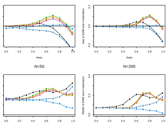
The results from our Monte Carlo analysis of the MA(1) model withσ2= 1and known (case I) are presented in Figures 1 and 2 and Table 1. Figures 1 and 2 present the biases (upper panels) and the RMSE (lower panels) values of the different estimators based on AR(3) and AR(8) auxiliary models, respectively, for n= 50(on the left) and n= 200(on the right). As expected, the ML estimator shows the best performance. No simulation-based estimator uniformly dominates in terms of bias or RMSE. Forn= 50,the II estimators perform the best in terms of bias forθ <0.5,the IL estimator has the best overall performance and the EL estimator has the worst performance. Interestingly, the biases of the II estimators display a hump-shaped pattern for 0.5 < θ <1, peaking at θ near 0.8. The IA estimator for the MA(1) model does not seem to exhibit the bias reduction qualities shown by Gouriéroux et al. (2001) and Duffee and Stanton (2007) for the AR(1) model. When θ
is near the noninvertibility region, we obtain similar results to Ghysels et al. (2003); that is, the EMM estimators exhibit larger biases than the II estimators. However, our results show that the IA and IM estimators show greater biases than the EMM estimators for θ near 0.8. In terms of RMSE, the IL and EL estimators outperform the other estimators. For n = 200, all estimators except EA perform similarly forθ <0.5and the II estimators again display hump-shaped behavior forθvalues near0.8. The EL shows the lowest RMSE except forθat the boundary. Overall, the IL estimator performs the best in terms of bias and the EL estimator performs best in terms of RMSE. Interestingly, the IA and IM estimators are nearly identical in terms of bias and RMSE. Given the
N=50
theta
bias of EMM and II estimator
s 0.0 0.2 0.4 0.6 0.8 1.0 -0 .2 0.0 0 .2 N=200 theta
bias of EMM and II estimator
s 0.0 0.2 0.4 0.6 0.8 1.0 -0 .2 0.0 0 .2 N=50 theta R M
SE of EMM and II estimator
s 0.0 0.2 0.4 0.6 0.8 1.0 0.0 0 .2 0.4 N=200 theta R M
SE of EMM and II estimator
s 0.0 0.2 0.4 0.6 0.8 1.0 0.0 0 .2 0.4
Figure 1: Biases (on the top) and RMSE (on the bottom) of the EL (empty triangles), EA (filled triangles), IL (empty squares), IA (squares with crosses), IM (filled squares), and ML (filled circles) estimators of a MA(1) process withθ= 0,0.1, . . . ,0.9,0.99based on AR(3) auxiliary models.
computational advantage of the IA estimator, it is to be preferred over the IM estimator6.
Table 1 presents the case I empirical rejection frequencies of nominal5%and1%LR-type tests for the null hypothesis H0 :θ = 0.5,0.6, . . . ,0.9 based on AR(3) and AR(8) auxiliary models for samples of size n= 50 and n = 200. The empirical rejection frequencies of the overidentification tests mirror those of the coefficient tests and are therefore omitted. For both sample sizes and all values of θ, the LR test based on the ML estimator is correctly sized. In general, the size distortions for the EMM and II estimators are larger with the AR(8) model and the tests based on the II estimators have about half the size distortion as the tests based on the EMM estimators.
6
For the case II (σ2= 1and estimated) simulations, the bias and RMSE results forθare qualitatively similiar to the case I simulations and are therefore omitted.
N=50
theta
bias of EMM and II estimator
s 0.0 0.2 0.4 0.6 0.8 1.0 -0 .2 0.0 0 .2 N=200 theta
bias of EMM and II estimator
s 0.0 0.2 0.4 0.6 0.8 1.0 -0 .2 0.0 0 .2 N=50 theta rm
se of EMM and II estimator
s 0.0 0.2 0.4 0.6 0.8 1.0 0.0 0 .2 0.4 N=200 theta rm
se of EMM and II estimator
s 0.0 0.2 0.4 0.6 0.8 1.0 0.0 0 .2 0.4
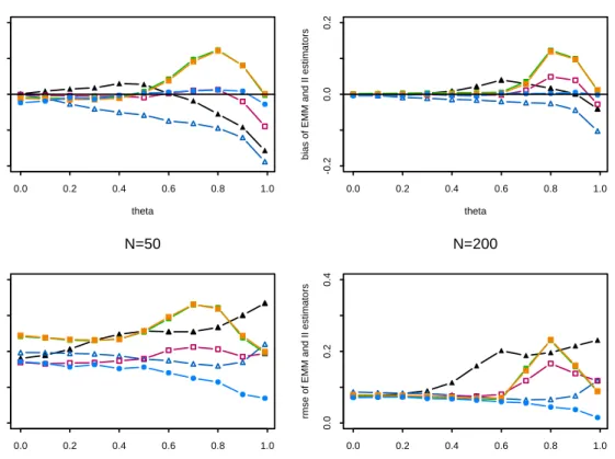
Figure 2: Biases (on the top) and RMSE (on the bottom) of the EL (empty triangles), EA (filled triangles), IL (empty squares), IA (squares with crosses), IM (filled squares), and ML (filled circles) estimators of a MA(1) process withθ= 0,0.1, . . . ,0.9,0.99based on AR(8) auxiliary models.
Interestingly, the results based on the non-simulation based EMM estimator are very similar to the simulation-based II estimators. The empirical rejection frequencies of the tests based on the EL and EA estimators are stable across θ whereas the tests based on the EN and II estimators tend to decline as θ approaches unity. The poor performance of the EN and II tests for θ near unity occurs because the binding function is not injective (one-to-one) aroundθ= 1.For the AR(8) model withn= 50,the tests based on the EMM estimators are substantially size distorted for all values ofθ:the 5% tests have empirical sizes around 44%. These large size distortions imply highly inaccurate confidence intervals formed by inverting the LR-type tests. The larger size distortions of the tests based on the AR(8) auxiliary model with n = 50 arises because the efficient weight
α= 0.05 α= 0.01 θ m ML EN EL EA IL IA IM ML EN EL EA IL IA IM n= 50 n= 50 0.5 3 0.05 0.10 0.17 0.17 0.08 0.09 0.09 0.01 0.03 0.09 0.09 0.03 0.03 0.03 8 0.20 0.44 0.43 0.22 0.24 0.20 0.11 0.33 0.32 0.11 0.13 0.10 0.6 3 0.05 0.08 0.17 0.17 0.08 0.06 0.09 0.01 0.02 0.09 0.08 0.02 0.02 0.02 8 0.21 0.43 0.43 0.20 0.21 0.22 0.10 0.33 0.32 0.10 0.11 0.11 0.7 3 0.06 0.06 0.16 0.15 0.06 0.04 0.05 0.01 0.01 0.08 0.08 0.01 0.01 0.01 8 0.20 0.43 0.44 0.20 0.19 0.23 0.10 0.32 0.32 0.08 0.08 0.11 0.8 3 0.04 0.05 0.16 0.15 0.03 0.05 0.03 0.01 0.02 0.09 0.08 0.01 0.01 0.01 8 0.16 0.43 0.45 0.15 0.16 0.15 0.06 0.32 0.32 0.06 0.07 0.06 0.9 3 0.02 0.05 0.18 0.17 0.04 0.05 0.03 0.01 0.02 0.11 0.08 0.02 0.01 0.01 8 0.09 0.42 0.43 0.08 0.09 0.09 0.04 0.31 0.32 0.04 0.04 0.04 n= 200 n= 200 0.5 3 0.06 0.05 0.09 0.06 0.05 0.06 0.04 0.01 0.02 0.03 0.01 0.02 0.01 0.01 8 0.08 0.15 0.12 0.08 0.09 0.07 0.03 0.08 0.06 0.02 0.02 0.02 0.6 3 0.05 0.05 0.09 0.06 0.04 0.05 0.05 0.01 0.01 0.03 0.01 0.00 0.02 0.00 8 0.07 0.14 0.12 0.07 0.07 0.08 0.02 0.07 0.05 0.02 0.02 0.02 0.7 3 0.06 0.05 0.07 0.05 0.04 0.04 0.04 0.01 0.01 0.03 0.01 0.00 0.00 0.01 8 0.07 0.13 0.11 0.09 0.08 0.07 0.02 0.06 0.04 0.03 0.02 0.02 0.8 3 0.04 0.02 0.07 0.04 0.02 0.02 0.03 0.01 0.00 0.03 0.01 0.00 0.01 0.00 8 0.07 0.12 0.11 0.08 0.07 0.08 0.01 0.05 0.04 0.02 0.02 0.01 0.9 3 0.06 0.02 0.07 0.05 0.02 0.03 0.02 0.02 0.00 0.04 0.02 0.01 0.00 0.00 8 0.03 0.13 0.12 0.03 0.03 0.00 0.01 0.05 0.03 0.01 0.01 0.00
Table 1: Empirical rejection frequencies of LR-type coefficient tests.
matrices are not accurately estimated in small samples. Forn= 200,the size distortions of all tests drop substantially but the EMM tests still exhibit a moderate amount of size distortion. The 5% tests based on the EMM estimators have empirical rejection rates around 15% for all values ofθ.
4
Saddlepoint Coe
ffi
cient Tests for EMM and II Estimators
The LR-type test statistics described in subsection 2.5 are based onfirst order asymptotic theory. Asymptotic normality of EMM and II estimators imply that the LR-type statistics defined in (28) are asymptotically χ2-distributed with an absolute error of order n−1/2. The χ2 approximation is then used to compute p-values for a hypothesis test. However, as illustrated by the Monte Carlo results of the previous section, p-values obtained using the χ2 approximation can be highly
inaccurate for small to moderate sample sizes. The aim of this section is to construct coefficient test statistics based on EMM and II such that the distribution of the statistics can be approximated by a χ2 distribution with a relative error of order n−1 or n−1/2. As a result, for these tests, χ2 p-values are expected to be more accurate in small samples.
To improve the accuracy of the asymptotic approximation to the distribution of estimators and test statistics, high-order approximation methods have been proposed. The most frequently used are Edgeworth expansions (cf., for instance, Feller, 1971) and saddlepoint approximations (Daniels, 1954). The superiority of the saddlepoint approximation for tail probabilities, which are the quantities of interest for inference tests and confidence intervals, when compared to the Edgeworth expansion is shown, for instance, in Barndorff-Nielsen and Cox (1989) and Field and Ronchetti (1990).
Our proposed saddlepoint tests of hypotheses on coefficients estimated by EMM/II estimators is based on the fact that we can associate an EMM/II estimator with an asymptotically equivalent M-estimator defined by the influence function of the EMM/II estimator, which allows us to use the saddlepoint coefficient test for M-estimators introduced by RRY.
4.1
RRY Coe
ffi
cient Tests for
M
-Estimators
Let {Xi}i=1,...,n be an i.i.d. sample of random vectors with common range X and distributionFθ with θ∈ Rp. Define theM-functional T that for a given distributionF associates the parameter
T(F)∈Rp defined by
EF
£
ψ(X, T)¤= 0,
where the score ψ is assumed to be a smooth function from X ×Rp to Rp.Consider a sample of observations{xi}i=1,...,n and define the empirical distributionFn as
Fn(x) = 1 n n X i=1 ∆xi(x), (36)
where ∆xi denotes the pointmass distribution, the probability measure which gives mass 1 to xi. The M-functional evaluated at the empirical distribution Fnis Tn=T(Fn) defined by
EFn £ ψ(X, T)¤= 1 n n X i=1 Z ψ(x, T)d∆xi(x) = 1 n n X i=1 ψ(xi, T).
Hence, theM-estimator ofθ isTn(X1, . . . , Xn) =T(Fn)(X1, . . . , Xn)defined by n
X
i=1
ψ(Xi, Tn) = 0. (37)
To simplify the notation, hereafter we denote the statistic Tn ≡Tn(X1, . . . , Xn) and its observed value bytn≡Tn(x1, . . . , xn).
Using the M-estimator Tn,we would like to test hypotheses of the formH0 : q(θ) =η0, where
q is a smooth function from Rp toRp1.
4.1.1 Analytical RRY Test
RRY considered the case where the cumulant generating function of the vector of scores exists and underH0 : q(θ) =η0,for a smooth functionq fromRp toRp1,is defined by
Kψ(λ, θ) = logEFθ(η0)
£
eλ0ψ(X,θ)¤. (38) Under the assumption that the density of the M-estimator exists and has a saddlepoint approxi-mation as given in Field (1982), RRY derived a saddlepoint approxiapproxi-mation to the density ofq(Tn) and proposed the test statistic
2nh(q(Tn)), (39) where
h(y) = inf
{θ:q(θ)=y}supλ {−Kψ(λ;θ)}. (40) Hereafter, we refer to the statistic (39) as theanalytical RRY test statistic. Using the saddlepoint approximation to the density of q(Tn), RRY showed that under regularity conditions the statistic (39) is χ2(p1) distributed with a relative error of order n−1 under H0. As a result, p-values for the saddlepoint test (39) based on the χ2 distribution are expected to be more accurate in finite samples than those for the Wald or LR-type tests whose approximations have absolute error or order
n−1/2.According to RRY, these results can be extended to the case when Xi are not identically distributed.
Simple Hypothesis
θ=θ0. In this case, the analytical RRY test statistic is2nh(Tn),where the functionh is simply h(y) = sup λ {− Kψ(λ, y)} (41) withKψ(λ, θ) = logEFθ0 h
eλ0ψ(X,θ)i.In the case when the model belongs to the exponential family
fθ(x) =c(θ)eθ
0l(x)
andTnis a ML estimator it is straightforward to show that2nh(Tn)is equivalent to the log-likelihood ratio statistic.
Composite Hypothesis
Suppose thatθ= (θ01, θ02)0,θ1∈Rp1 andθ2 ∈Rp2. Consider the case whenq(θ) =θ1 and we are interested in testing the hypothesisH0 : θ1 =θ1 0. In this case, the analytical RRY test statistic is 2nh(Tn1),where Tn= (Tn01, Tn02)0 and the functionh is defined by
h(y) = inf θ2 sup λ {− Kψ(λ,(y, θ2))} (42) with Kψ(λ, θ) = logEF(θ1 0,θ2) h
eλ0ψ(X,θ)i. Essentially, the nuisance parameter θ2 is concentrated out of Kψ(λ, y) when forming the test statistic for H0 : θ1 = θ1 0.A confidence set for θ1 may be constructed by inverting 2nh(Tn1) using a χ2(p1) critical value. Specifically, a (1−α)·100% confidence set forθ1 is
{θ10: 2nh(Tn1))≤χ21−α(p1)}. (43)
4.1.2 Empirical RRY Test
In practice, the distributionFθmay be unknown and even when it is known, the cumulant generat-ing function may not exist. For these purposes, RRY defined an empirical version of the test based on an exponentially weighted empirical cumulant generating function that imposesH0 : q(θ) =η0. Define an empirical distribution Fˆ0 consistent with the null hypothesis:
ˆ F0(x) = Pn i=1eβ(η0) 0ψ(xi,θ(η0)) ∆xi(x) Pn i=1eβ(η0)0ψ(xi,θ(η0)) ,
whereβ=β(η0),θ=θ(η0)are chosen to minimize the backward Kullback—Leibler distance between the empirical distribution and the tilted empirical distribution subject to
see DiCiccio and Romano (1990). The solutions to this minimization are solutions of the equations ∂κ ∂β(β, θ) = 0, (44) q(θ) =η0, (45) ∂κ ∂θ(β, θ) = ∂q(θ)0 ∂θ γ , (46) where κ(β, θ) = log " 1 n n X i=1 eβ0ψ(xi,θ) #
and γ=γ(η0)is the Lagrange multiplier of the optimization problem. Notice that the saddlepoint
β(θ)in equation (44) is solution to the following optimization problem:
β(θ) =argmax
β (−κ(β, θ)). (47)
The empirical cumulant generating function is then defined by
Kψω(λ, θ) = logEFˆ0[eλ 0ψ(X,θ) ] = log n X i=1 eβ(η0)0ψ(xi,θ(η0)) Pn i=1eβ(η0) 0ψ(xi,θ(η0)) | {z } ωi Z eλ0ψ(x,θ)∆xi(x) = log n X i=1 ωieλ 0ψ(xi,θ) ,
which corresponds to a weighted empirical cumulant generating function where the weights are consistent with the null hypothesis. Theempirical RRY test is then defined by
2nˆh(q(Tn)), (48) with ˆ h(y) = inf {θ:q(θ)=y}supλ {− Kψω(λ, θ)}. (49) For this empirical version of the saddlepoint test, RRY did not prove that the relative error of theχ2 approximation is of ordern−1 but provided simulation experiments that indicated a relative error ofn−1. RRY also did not consider cases whereXi are not independent. Our simulations in Section 5, however, show that even in the case when the Xi are not independent but the scores follow a stationary and ergodic martingale difference sequence the χ2 approximation to the distribution of
the empirical RRY statistic (48) leads to more accurate inference than those obtained using theχ2 approximation to the distribution of an LR-type statistic.
Weights For the Simple Hypothesis
In the simple case whenq(θ) =θand the test hypothesis isH0 :θ=θ0, the empirical distribu-tion Fˆ0 is determined by the equations (44) and (45). The weights are then defined by
ωi = eβ(θ0)0ψ(xi,θ0) Pn i=1eβ(θ0) 0ψ(xi,θ0), whereβ(θ0)is defined by (47).
Weights For the Composite Hypothesis
Consider the case when q(θ) =θ1 and the test hypothesis isH0:θ1 =θ1 0. Equation (45)fixes thep1 parameters inθ1 and the parameters in θ2, determined by equations (44)-(46), are solutions to the following minimization problem
θ∗2 = min θ2 ³ −κ¡β(θ1 0, θ2),(θ1 0, θ2) ¢´ ,
whereβ(θ) is defined by (47). Indeed, the Lagrangian to this minimization problem is L(θ, γ) =−κ(β(θ), θ) +γ0(q(θ)−θ1 0),
and thefirst order conditions are
∂L ∂θ(θ, γ) =− ∂β(θ)0 ∂θ ∂κ ∂β(β(θ), θ) | {z } 0 +∂q(θ) 0 ∂θ γ= 0, ∂L ∂γ(θ, γ) =q(θ)−θ1 0= 0.
4.2
Asymptotically Equivalent M-Estimators for II and EMM Estimators
The EMM and II estimators considered in this paper are not defined as M-estimators of the form (37), so it is not obvious that the RRY tests can be applied. However, using properties of the influence functions (Hampel, 1974; Hampelet al., 1986) for EMM and II estimators we can associate asymptotically equivalentM-estimators and use the score function from theseM-estimators to form the RRY tests evaluated at the EMM/II estimates.The influence function for non-simulation-based II estimator defined in (6) has been derived by Genton and de Luna (2000), and for non-simulation-based EMM estimator (5) by Ortelli and Trojani (2005). To describe these influence functions, let Te be the functional associated with the auxiliary ML estimatorμ˜defined in (1). That is,μ˜ =Te(Fn)whereFnis the empirical distribution (36). Denote by TII the functional associated with the II estimators and TEMM the functional associated with the EMM estimators. Assume that Fisher consistency holds; that is, Te(Fθ) = μ
andTII(Fθ) =TEMM(Fθ) =θ. To economize on notation in what follows, letyandx denotey0 and
x−1, respectively. The influence functions of the EMM and II estimators based on arbitrary fixed weight matricesΩ and Σare, respectively:
IF(y, TEMM, Fθ) =− ¡ Mθ0ΣMθ ¢−1 Mθ0ΣMμIF(y,T , Fe θ), (50) IF(y, TII, Fθ) = µ ∂μ(θ)0 ∂θ0 Ω ∂μ(θ) ∂θ0 ¶−1 ∂μ(θ)0 ∂θ0 ΩIF(y,T , Fe θ), (51) whereIF(y,T , Fe θ) is the influence function of the auxiliary estimatorμ˜. For the case in which the auxiliary estimator μ˜ is anM-estimator defined by Pt∂μ∂f˜(yt;xt−1,μ˜) = 0, the influence function of the auxiliary estimator μ˜ is given by
IF(y,T , Fe θ) =−Mμ−1
∂f˜
∂μ(y;x, μ(θ)). (52)
Since the EMM and II estimators based on the optimal weight matricesΣ∗ andΩ∗ are asymp-totically equivalent under suitable regularity conditions, it turns out that influence functions of the optimal EMM and II estimators are also equivalent. This result follows directly from (20) and (27). A Fisher consistent estimator is asymptotically equivalent to the M-estimator defined by the influence function of the Fisher consistent estimator (see Hampelet al., 1986, p. 231; Newey and McFaddan, 1994; Czellar and Ronchetti, 2008). Denote byθˆaeII(Ω) and θˆEMMae (Σ) theM-estimators that are asymptotically equivalent to the II and EMM estimators using the weight matrices Ωand
Σ, respectively. Using (50)-(52), θˆae
II(Ω)and θˆaeEMM(Σ) are defined by the first order conditions:
X t ζII(yt,θˆIIae(Ω),Ω) = 0 and X t ζEMM(yt,θˆEMMae (Σ),Σ) = 0, (53) where ζII(y, θ,Ω) = ∂μ(θ)0 ∂θ ΩM −1 μ ∂f˜ ∂μ(y;x, μ(θ)), (54)
ζEMM(y, θ,Σ) =Mθ0Σ
∂f˜
∂μ(y;x, μ(θ)). (55)
The score functions (54) and (55) are identical when evaluated at the optimal weight matricesΩ∗
and Σ∗ given by (20), respectively, and become
ζ∗(y, θ,I−1) =Mθ0I−1 ∂
˜
f
∂μ(y;x, μ(θ)). (56)
In most applications the quantities μ(θ),Mμ, Mθ,and I in the score functions (54) - (56) are unknown and must be estimated. We note that the asymptotically equivalent M-estimator based on an estimated version of the optimal score (56) is equivalent to the non-simulation based EMM estimator defined in (5) with Σ˜ =Ie−1. Indeed, thefirst order conditions from (5) are
c Mˆ0 θaeIe− 1 n g˜n(ˆθae) = 0, where c Mθˆae = ∂ ∂θ0 à 1 n−m n X t=m+1 ∂f˜ ∂μ(yt;xt−1, μ(ˆθ ae)) ! , (57)
which is of the formPnt=m+1ζˆ∗(yt,θˆae,Ien−1) = 0withζˆ∗(yt,θˆae,Ien−1) =Mcθ0ˆaeIb−
1 n ∂ ˜ f ∂μ(yt;xt−1, μ(ˆθ ae)).
4.3
Empirical RRY Tests Based on Asymptotically Equivalent M-Estimators
Using the M-estimator score functions (54) and (55), analytic RRY tests for the hypothesis H0 :q(θ) = η0 ∈Rp1 based on the asymptotically equivalentM-estimates defined by (53) are given by (39) with Tn replaced by θˆaeII(Ω) or θˆEMMae (Σ), respectively. Under the conditions stated in RRY, these tests are then χ2(p1)-distributed with a relative error of order n−1 under H0. Given that we associate the asymptotically equivalent M-estimators with the simulation-based EMM and II estimators, we propose the following empirical RRY tests for EMM and II:
2 nS S+ 1 ˆ h(q(ˆθSi( ˜Σ)), i= EL,EA, (58) 2 nS S+ 1 ˆ h(q(ˆθSi( ˜Ω)), i= IL,IM,IA. (59)
where the functionˆhis defined in (49) and uses the score functions (55) and (54) for EMM and II, respectively. If the efficient EMM or II estimators are computed then the score function (56) may be used in the construction of the test for either estimator. We expect that inference based on the
ˆ θSni ζ(y, θ) μ(θ) Mθ Mμ EL M0 θΣ ∂f˜ ∂μ(y;x, μ(θ)) μ˜LS(θ) ∂θ∂0˜gSn(θ, μ) − EA Mθ0Σ∂∂μf˜(y;x, μ(θ)) μ˜AS(θ) ∂θ∂0S1 PsS=1g˜ns(θ, μ). − IL ∂μ∂θ(θ0)0ΩMμ−1 ∂f˜ ∂μ(y;x, μ(θ)) μ˜LS(θ) − ∂μ∂0g˜Sn(θ, μ) IA ∂μ∂θ(θ0)0ΩMμ−1∂μ∂f˜(y;x, μ(θ)) μ˜AS(θ) − ∂μ∂0S−1PSs=1g˜ns(θ, μ) IM ∂μ∂θ(θ0)0ΩMμ−1 ∂f˜ ∂μ(y;x, μ(θ)) μ˜MS(θ) − ∂ ∂μ0S−1 PS s=1g˜ns(θ, μ) Table 2: Approximations of limit quantities needed to implement empirical RRY tests for EMM and II estimators.
empirical RRY tests (58)-(58) to be more accurate in finite samples than inference based on the classical LR-type statistics (28). We provide Monte Carlo evidence to back up this claim in the next section.
We make the following remarks regarding the implementation of the empirical RRY tests for EMM and II estimators:
1. When the empirical RRY tests are evaluated at the simulation-based EMM or II estimates, they must by scaled by SS+1 to account for the increase in variability due to simulations.
2. The tests in (58) and (59) are defined for arbitrary weight matrices, not just the efficient weights matrices required for computing the LR-type tests.
3. The binding function, μ(θ), and the limit quantities, Mθ and Mμ, needed for the computation of the empirical RRY tests are typically unknown, but can be approximated using the pseudo-data generated for the computation of the EMM and II estimators as follows. For the RRY tests using EL estimates, replaceμ(θ)byμ˜L S(θ), and replaceEFθ h ∂f˜ ∂μ(y;x, μ) i
inMθ byg˜Sn(θ, μ). For the RRY test using EA estimates, replaceμ(θ)byμ˜A
S(θ)and replaceEFθ h ∂f ∂μ(y;x, μ) i by S−1PS s=1g˜ns(θ, μ). For the RRY test using IL, IM and IA estimates, replaceμ(θ)byμ˜LS(θ),μ˜MS(θ),andμ˜AS(θ)defined by (13), (14) and (19), respectively. The quantityEFθ
h
∂2f˜
∂μ∂μ0(y;x, μ)
i
can be replaced by ∂μ∂0g˜Sn(θ, μ) for IL, and by ∂μ∂0S−1PsS=1˜gsn(θ, μ)for IA and IM. These approximations are summarized in Table 2.
4. The derivative of the binding function, ∂μ∂θ(θ),can be calculated numerically, for example using Ridders method of polynomial extrapolation.
5
Finite Sample Performance of Empirical RRY Tests for EMM
and II
To illustrate thefinite sample performance of the empirical RRY tests based on the optimal EMM and II estimators, we utilize the Monte Carlo set-up from subsection 3.1. Table 3 presents the empirical rejection frequencies of nominal 5% and 1% tests for the null hypothesis H0 : θ = 0.5,0.6, . . . ,0.9 based on 1,000 Monte Carlo replications of (32) with σ2 = 1 and known. To compute the tests for the asymptotically equivalent M-estimator (denoted EN in Table 3), we use (56) with I estimated using (23) and Mθ estimated using (57). To compute the tests for the simulation-based estimators, theM-estimator score functions (55) and (54) are approximated using the formulas described in Table 2.7 In contrast to the classical LR-type tests reported in Table 1,
the empirical RRY tests show much less size distortion especially for the AR(8) auxiliary model.
Importantly, our proposed RRY tests (58) and (59) using the simulation-based estimators perform similarly to the test based on the non-simulation based asymptotically equivalentM-estimator. For the AR(3) auxiliary model, the tests based on the simulation-based EMM estimators show almost no size distortion whereas the tests based on the asymptotically equivalentM-estimator and the II estimators are slightly undersized and the size distortion tends to increase as θ approaches unity. For the AR(8) auxiliary model, the tests based on the EMM estimates display more size distortion than the tests based on the other estimators forn= 50but the size distortion is mostly eliminated whenn= 200.The tests based on the EMM estimators are computationally faster and numerically more stable than those based on the II estimators. The numerical instability mainly occurs in the computation of the derivative of the binding function when evaluating the score function (54).
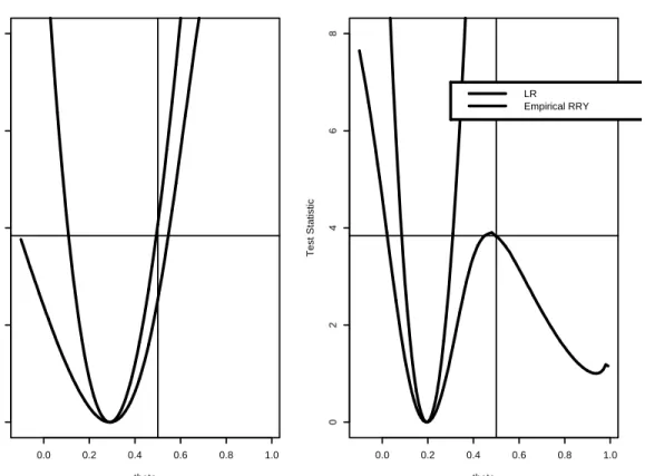
To illustrate the confidence sets for θ obtained by inverting the LR-type and empirical RRY test statistics based on the EL estimator, Figure 3 shows (28) and (58) as functions of θ0 from a representative simulated sample from (32) of size n= 50withθ= 0.5.The EL estimates from the AR(3) and AR(8) auxiliary models are 0.255 and 0.212, respectively. The horizontal line in the figures represents the 95 percent quantile from the χ2(1) distribution, and the corresponding 95 percent confidence sets consist ofθ0 values such that the test statistics lie below the horizontal line. For both auxiliary models, the LR-type test is quadratic and symmetric in θ but the 95 percent confidence intervals do not include the true value θ = 0.5. The empirical RRY test, in contrast, is asymmetric in θ. For the AR(3) model the 95 percent confidence interval is considerably wider than the LR-type confidence interval and includes the true value θ= 0.5.For the AR(8) auxiliary
7
We also computed the empirical RRY tests using analytic values forμ(θ), Mθ andMμ.This greatly reduced the computation time of the tests and the results were almost identical.
α= 0.05 α= 0.01 θ m EN EL EA IL IA IM EN EL EA IL IA IM n= 50 n= 50 0.5 3 0.03 0.05 0.04 0.04 0.04 0.04 0.00 0.01 0.01 0.01 0.01 0.01 8 0.05 0.11 0.10 0.08 0.07 0.08 0.01 0.03 0.03 0.01 0.01 0.01 0.6 3 0.02 0.05 0.05 0.02 0.02 0.02 0.00 0.01 0.01 0.00 0.01 0.01 8 0.05 0.11 0.09 0.07 0.08 0.07 0.00 0.03 0.02 0.01 0.01 0.01 0.7 3 0.02 0.05 0.05 0.02 0.02 0.02 0.00 0.01 0.01 0.00 0.00 0.00 8 0.04 0.10 0.10 0.04 0.03 0.03 0.00 0.02 0.02 0.00 0.00 0.00 0.8 3 0.01 0.05 0.06 0.02 0.02 0.02 0.00 0.01 0.01 0.00 0.00 0.00 8 0.03 0.11 0.09 0.03 0.03 0.02 0.00 0.02 0.02 0.00 0.00 0.00 0.9 3 0.00 0.05 0.07 0.02 0.02 0.02 0.00 0.01 0.00 0.00 0.00 0.00 8 0.03 0.10 0.11 0.04 0.03 0.03 0.00 0.03 0.02 0.01 0.01 0.01 n= 200 n= 200 0.5 3 0.04 0.06 0.04 0.05 0.03 0.04 0.02 0.02 0.00 0.02 0.01 0.01 8 0.05 0.08 0.07 0.06 0.05 0.05 0.01 0.02 0.02 0.01 0.01 0.01 0.6 3 0.03 0.05 0.04 0.05 0.03 0.02 0.01 0.01 0.00 0.01 0.00 0.00 8 0.05 0.08 0.06 0.06 0.05 0.05 0.01 0.01 0.01 0.02 0.01 0.01 0.7 3 0.02 0.04 0.04 0.02 0.01 0.01 0.00 0.01 0.00 0.01 0.00 0.00 8 0.05 0.08 0.06 0.06 0.05 0.04 0.01 0.01 0.01 0.01 0.01 0.01 0.8 3 0.02 0.05 0.04 0.02 0.01 0.01 0.00 0.01 0.01 0.01 0.00 0.00 8 0.02 0.07 0.06 0.03 0.02 0.02 0.00 0.01 0.01 0.00 0.00 0.00 0.9 3 0.01 0.05 0.05 0.02 0.01 0.01 0.00 0.01 0.01 0.01 0.02 0.01 8 0.03 0.08 0.06 0.02 0.02 0.02 0.00 0.01 0.01 0.00 0.00 0.00 Table 3: Empirical rejection frequencies of empirical RRY tests for EMM and II estimators.
AR(3) auxiliary model theta Test Statistic 0.0 0.2 0.4 0.6 0.8 1.0 02 46 8
AR(8) auxiliary model
theta Test Statistic 0.0 0.2 0.4 0.6 0.8 1.0 02 46 8 LR Empirical RRY
Figure 3: LR-type and empirical RRY confidence sets for θ from representative case I simulation withn= 50.
model, the confidence set is disconnected due to a local maximum of the statistic nearθ= 0.5but still contains the true value. The confidence sets based on the two statistics forn= 200are almost identical and shows that large sample inference based on the empirical RRY test is essentially the same as that based on the LR-type statistic.
From the case II simulations, we computed empirical rejection frequencies of the composite tests for H0 : θ = θ0 and H0 : σ2 = 1. Since the case I simulations show that the empirical rejection frequencies are stable across θ and large size distortions only occur for the EMM tests,
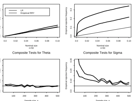
we set θ = 0.5 and only computed tests based on the EL estimator. The top panel of Figure 4 showsp-values plots of the LR-type and empirical RRY tests based on the AR(3) auxiliary model for n = 50, and the bottom panel shows empirical rejection frequencies of nominal five percent
Composite Tests for Theta n=50 Nominal size Empir ical r e jection fr equency 0.0 0.02 0.04 0.06 0.08 0.10 0.0 0 .1 0.2 0 .3 LR Empirical RRY
Composite Tests for Sigma
n=50 Nominal size Empir ical r e jection fr equency 0.0 0.02 0.04 0.06 0.08 0.10 0.0 0 .1 0.2 0 .3
Composite Tests for Theta
Sample size, n Empir ical r e jection fr equency 100 200 300 400 500 0.0 0 .10 0 .20 0 .30
Composite Tests for Sigma
Sample size, n Empir ical r e jection fr equency 100 200 300 400 500 0.0 0 .10 0 .20 0 .30
Figure 4: Top: p-values plots of composite tests. Bottom: Empirical rejection frequencies of nominal 5 percent tests as a function of sample size.
tests, based on the AR(3) auxiliary model, as a function of sample size. In contrast to the case I simulations, the LR-type and empirical RRY tests for H0 :θ = θ0 are essentially correctly sized. However, the LR-type test forH0 :σ2 = 1displays about twice the size distortion as the empirical RRY test for small samples.
Figure 5 shows finite sample size adjusted power of the 5% LR-type and empirical RRY tests, based on the EL estimator with AR(3) and AR(8) auxiliary models, of the null hypothe-sis H0 : θ = 0.5 against the alternative H0 : θ 6= 0.5 when the true value satisfies θ = 0.5 +δ (δ =±0.1,0.2,0.3,0.4) using 1,000Monte Carlo replications. We present results only for the EL estimator from the case I simulations since thefinite sample size distortions of the LR-type test were largest for this estimator. Results for the other estimators are similar and are therefore omitted.
AR(3) Auxiliary Model, N=50 theta Empir ical r e jection fr equency of 5% test 0.2 0.4 0.6 0.8 0.0 0 .4 0.8
AR(3) Auxiliary Model, N=200
theta Empir ical r e jection fr equency of 5% test 0.2 0.4 0.6 0.8 0.0 0 .4 0.8
AR(8) Auxiliary Model, N=50
theta Empir ical r e jection fr equency of 5% test 0.2 0.4 0.6 0.8 0.0 0 .4 0.8
AR(8) Auxiliary Model, N=200
theta Empir ical r e jection fr equency of 5% test 0.2 0.4 0.6 0.8 0.0 0 .4 0.8
Figure 5: Size-adjusted power of nominal 5% EL LR-type (squares) and EL empirical RRY (trian-gles) tests for H0 :θ= 0.5versus H0 :θ6= 0.5.
In general, the size-adjusted power of the empirical RRY test is very similar to LR-type test. For
n = 50,the empirical RRY test has the same power as the LR-type test for θ <0.5 and smaller power forθ >0.5.Forn= 200,the empirical RRY test has nearly the same size-adjusted power as the LR-type test for all values of θ. Hence, use of the empirical RRY test for the simulated-based EMM and II estimators results in more accurate inference in small samples without a loss in power.
6
Conclusion
EMM and II are widely used simulation-based estimation techniques. Finite sample comparisons have shown that point estimates based on EMM and II are often similar, but that interval estimates
and empirical rejection frequencies of coefficient and overidentification tests based on asymptotic theory can be substantially different with II giving more reliable results than EMM. This has led several researchers (e.g., Ghysels et al., 2003, Duffee and Stanton, 2007) to advocate the use of II over EMM. Our proposed empirical RRY tests provide improved inference for EMM and II in small samples. For the MA(1) model, we show that the large size distortions of the classical LR-type tests for EMM are greatly reduced by the empirical RRY tests without suffering a loss in power. Our results have important practical relevance as they show that accurate finite sample inference can be obtained from EMM estimates.
Our finite sample results were illustrated using a simple MA(1) model. In future research we plan to apply the empirical RRY tests to more realistic models used infinance including stochastic volatility and continuous-time diffusion models. We also plan to implement the RRY tests for EMM estimation based on seminonparametric auxiliary models.
We have shown that the saddlepoint tests can give accurate finite sample inference for EMM and II based on correctly specified models. If the observed data is contaminated in some way or if the model is slightly misspecified, then the EMM and II estimators can give misleading results and the saddlepoint tests may not provide improved inference. However, Genton and Ronchetti (2003) and Ortelli and Trojani (2005) show that II and EMM can be made robust to contamination and certain types of misspecification. It is natural then to consider applying the saddlepoint tests for EMM and II to the robust versions over these estimators. This extension is explored in Czellar and Ronchetti (2008).
References
[1] Bansal, R., Gallant, A.R., Hussey, R., and Tauchen, G. (1993), Computational Aspects of Nonparametric Simulation Estimation, in D.A. Belsley, ed., Computational Techniques for Econometrics and Economic Analysis, Boston: Kluwer.
[2] Bansal, R., Gallant, A.R., Hussey, R., and Tauchen, G. (1995), “Nonparametric Estimation of Structural Models for High-Frequency Currency Market Data”,Journal of Econometrics,66, 251-287.
[3] Barndorff-Nielsen, O. E. and Cox, D. R. (1989), Asymptotic Techniques for Use in Statistics, London: Chapman & Hall.
[4] Chumacero, R. (1997), “Finite sample properties of the Efficient Method of Moments”,Studies in Nonlinear Dynamics and Econometrics,2, 35—51.
[5] Chumacero, R. (2001), “Estimating ARMA Models Efficiently”,Studies in Nonlinear Dynam-ics and EconometrDynam-ics,5, 103—114.
[6] Czellar, V. and Ronchetti, E. (2008), “Second-order Accurate and Robust Indirect Inference”, unpublished manuscript, Department of Econometrics, University of Geneva.
[7] Daniels, H.E. (1954), “Saddlepoint Approximations in Statistics”,The Annals of Mathematical Statistics,25, 631—650.
[8] de Luna, X. and Genton, M. G. (2001), “Robust Simulation-Based Estimation of ARMA Mod-els”,Journal of Computational and Graphical Statistics,10, 370—387.
[9] DiCiccio, T.J., and Romano, J.P. (1990), “Nonparametric Confidence Limits by Resampling Methods and Least Favorable Families,”International Statistical Review, 58, 59-76.
[10] Duffee, G. R. and Stanton, R. H. (2007), “Evidence on Simulation Inference for Near Unit-Root Processes with Implications for Term Structure Estimation”,Journal of Financial Economet-rics, 1-35.
[11] Feller, W. (1971), An Introduction to Probability Theory and its Applications, vol. 2, Wiley, New York.
[12] Field, C.A. (1982), “Small Sample Asymptotic Expansions for Multivariate M-estimates,” Annals of Statistics, 10, 672-689.
[13] Field, C. and Ronchetti, E. (1990), Small Sample Asymptotics, Institute of Mathematical Statistics - Monograph Series, Hayward (CA).
[14] Gallant, A. R., and Tauchen, G (1992), “A Nonparametric Approach to Nonlinear Time Series Analysis: Estimation and Simulation,” in D. Brillinger, P. Caines, J. Geweke, E. Parzen, M. Rosenblatt, and M.S. Taqqu (eds.) New Directions in Time Series Analysis, Part II. New York: Springer-Verlag, 71-92.
[15] Gallant, A. R. and Tauchen, G. (1996), “Which Moments to Match?”, Econometric Theory,
12, 657—681.
[16] Gallant, A. R. and Tauchen, G. (2001a), “SNP: A Program for Nonparametric Time Series Analysis”,manuscript, University of North Carolina.
[17] Gallant, A. R. and Tauchen, G. (2001b), “EMM: A Program for Efficient Method of Moments Estimations”,manuscript, University of North Carolina.
[18] Gallant, A. R. and Tauchen, G. (2002), “Simulated Score Methods and Indirect Inference for Continuous-time Models,” forthcoming in Y. Ait-Sahalia (editor) Handbook of Financial Econometrics, Elsevier Science Ltd.
[19] Genton, M. G. and de Luna, X. (2000), “Robust Simulation-Based Estimation”, Statistics & Probability Letters,48, 253—259.
[20] Genton, M. G. and Ronchetti, E. (2003), “Robust Indirect Inference”,Journal of the American Statistical Association,98, 67—76.
[21] Ghysels, E., Khalaf, L. and Vodounou, C. (2003), “Simulation Based Inference in Moving Average Models”,Annales D’Économie et de Statistique, 69, 85-99.
[22] Gouriéroux, C., Monfort, A. and Renault, E. (1993), “Indirect Inference”,Journal of Applied Econometrics,8, S85—S118.
[23] Gouriéroux, C., Renault, E. and Touzi, N. (2000), “Calibration by Simulation for Small Sample Bias Correction,” in Mariano, R., Schuerman, T. and Weeks, M.J. (eds), Simulation-Based Inference in Econometrics, Cambridge University Press.
[24] Hampel, F. R. (1974), “The Influence Curve and its Role in Robust Estimation”, Journal of the American Statistical Association,69, 383—393.
[25] Hampel, F. R., Ronchetti, E. M., Rousseeuw, P. J. and Stahel, W. A. (1986),Robust Statistics: The Approach Based on Influence Functions, John Wiley, New York.
[26] Hansen, L.P., Heaton, J.C. and Yaron, A. (1996), “Finite-Sample Properties of Some Alterna-tive GMM Estimators”,Journal of Business and Economic Statistics,14, 262-280.
[27] Michaelides, A. and Ng, S. (2000), “Estimating the Rational Expectations Model of Spec-ulative Storage: A Monte Carlo Comparison of Three Simulation Estimators”, Journal of Econometrics,96, 231-266.
[28] Newey, W.K. and West, K.D. (1987), “A Simple Positive Semidefinite Heteroskedasticity and Autocorrelation Consistent Covariance Matrix,”Econometrica, 55, 703-708.
[29] Newey, W.K., and McFadden, D. (1994), “Large Sample Estimation and Hypothesis Testing,” Chapter 36 in Engle, R.F., McFadden, D.L (eds), Handbook of Econometrics, Volume IV, Elsevier Science B.V.
[30] Ortelli, C. and Trojani, F. (2005), “Robust Efficient Method of Moments”,Journal of Econo-metrics,128, 69—97.
[31] Robinson, J., Ronchetti, E. and Young, G.A. (2003), “Saddlepoint Approximations and Tests Based on Multivariate M-estimators”, The Annals of Statistics, 4, 1154-1169.
[32] Smith, A. (1993), “Estimating Nonlinear Time Series Models Using Simulated Vector Autore-gressions”,Journal of Applied Econometrics,8, S63-S84.
[33] Zhou, H. (2001), “Finite Sample Properties of EMM, GMM, QMLE, and MLE for a Square-Root Diffusion Model”,Journal of Computational Finance,5, 89-122.
[34] Zivot, E. and Wang, J. (2005).Modeling Financial Time Series with S-PLUS, Second Edition, Springer-Verlag, New York.