This article has been accepted for publication and undergone full peer review but has not been through the copyediting, typesetting, pagination and proofreading process which may lead to differences between this version and the Version of Record. Please cite this article as doi: 10.1029/2019MS001924
Samadi S. (Orcid ID: 0000-0003-1494-6481)
Pourreza-Bilondi Mohsen (Orcid ID: 0000-0001-6922-6559)
Wilson Catherine, A.M.E. (Orcid ID: 0000-0002-7128-590X)
Bayesian Model Averaging with Fixed and Flexible Priors: Theory, Concepts, and Calibration Experiments for Rainfall-Runoff Modeling
S. Samadi1*,M. Pourreza-Bilondi 2, C. A. M.E Wilson 3, D. B. Hitchcock 4
1. Agricultural Sciences Department, Clemson University, USA.
2. Department of Water Engineering, University of Birjand, Birjand, Iran.
3. Hydro-environmental Research Centre, School of Engineering, Cardiff University, Cardiff, United Kingdom.
4. Department of Statistics, University of South Carolina, Columbia, USA. *Corresponding author: S. Samadi ([email protected])
Key Points:
1. Bayesian Model Averaging with fixed and flexible prior structures were applied to combine the posterior probability distribution of four hydrological models.
2. Custom prior inclusion and uniform prior induced a much sharper posterior median.
3. Putting a prior on both θ and g makes the analysis naturally adaptive and avoids the information paradox.
Abstract
This paper introduces for the first time the concept of Bayesian Model Averaging (BMA) with multiple prior structures, for rainfall-runoff modeling applications. The original BMA model proposed by Raftery et al. (2005) assumes that the prior probability density function (pdf) is adequately described by a mixture of Gamma and Gaussian distributions. Here we discuss the advantages of using BMA with fixed and flexible prior distributions. Uniform, Binomial, Binomial-Beta, Benchmark, and Global Empirical Bayes priors along with Informative Prior Inclusion and Combined Prior Probabilities were applied to calibrate daily streamflow records of a coastal plain watershed in the South-East USA. Various specifications for Zellner's g prior including Hyper, Fixed, and Empirical Bayes Local (EBL)
g priors were also employed to account for the sensitivity of BMA and derive the conditional pdf of each constituent ensemble member. These priors were examined using the simulation results of conceptual and semi-distributed rainfall-runoff models. The hydrologic simulations were first coupled with a new sensitivity analysis model and a parameter uncertainty algorithm to assess the sensitivity and uncertainty associated with each model. BMA was then used to subsequently combine the simulations of the posterior pdf of each constituent hydrological model. Analysis suggests that a BMA based on combined fixed and flexible priors provides a coherent mechanism and promising results for calculating a weighted posterior probability compared to individual model calibration. Furthermore, the probability of Uniform and Informative Prior Inclusion priors received significantly lower predictive error whereas more uncertainty resulted from a fixed g prior (i.e. EBL).
Plain Language Summary
This study presents a two-step procedure that includes model calibration of a range of hydrological models using DREAM (zs) algorithm, followed by ensemble prediction of streamflow using Bayesian Model Averaging (BMA) with various prior structures. The hydrological modeling simulations were first coupled with a new sensitivity analysis model and a parameter uncertainty algorithm to assess the sensitivity and uncertainty associated with each hydrologic model simulation. BMA was then used to subsequently combine the simulations on the most important parts of the posterior probabilities of each constituent hydrological model. Analysis suggests a BMA with fixed and flexible priors provides a coherent mechanism and promising results for calibrating a weighted posterior probability compared to individual model calibration. The hierarchy of prior distributions used in this study increased the flexibility of BMA fitting for daily streamflow simulation and reduced the dependence of posterior and predictive uncertainty (including model probabilities) on prior assumptions of hydrological modeling simulation.
1. Introduction
Model uncertainty is a critical problem that raises questions about the alternative modelling paradigm to simulate observed processes. Which set of the model approaches is appropriate to faithfully simulate and explain the variation in the observational records? How should one explicitly or implicitly evaluate the suitability of alternative models and characterize predictive uncertainty arising from different modeling assumptions? In addressing these questions, multi-model ensembles (MME) has become a popular alternative for probabilistic merging of simulations. By exploiting the information contained in multiple modeling structures, the MME approach is expected to provide better and more reliable estimates of forecast uncertainty. In the last decade, MME has gained popularity in different research disciplines including climatology (Grimitt and Mass, 2002; Barnston et al., 2003; Palmer et al., 2004; Raftery et al., 2005; Bao et al., 2010), public health (e.g. Thomson et al. 2006), and agriculture (e.g. Cantelaube and Terres 2005). In hydrology, MME has led to significant improvement in flow simulation and estimates of the forecast probability density function (pdf; e.g., Rajagopalan et al., 2002, 2005; Doblas-Reyes et al., 2005; Gneiting et al., 2005; Min and Hense, 2006; Duan et al. 2007; Rings et al., 2012; Madadgar and Moradkhani 2014; Najafi and Moradkhani, 2015; He et al., 2018; among others). The first attempt in using MME in hydrology used the simple average method (SAM), the weighted average method (WAM) and the neural network method (NNM) in simulation (Shamseldin et al., 1997). Fuzzy systems were also employed to combine the simulation results of different conceptual rainfall-runoff models in a flood forecasting study (Xiong et al., 2001). Subsequently a number of studies showed that ensemble simulations outperformed the best model if the aim was to use the outputs in
operational forecasting system (Butts et al.;2004; Georgakakos et al.,2004; Rajagopalan et al., 2005; Grantz et al., 2005).
The theoretical basis of MME was strengthened by the introduction of Bayesian Model Averaging (BMA), a statistical method of producing probabilistic forecasts from ensembles of regression models, accounting for model uncertainty within a Bayesian framework. An excellent overview of the theory behind BMA is given by Hoeting et al. (1999). Raftery et al. (2005) provided an early application of BMA to weather forecasting. BMA addresses uncertainty by calculating a weighted average of all potential model combinations (Feldkircher and Zeugner, 2009) and describes both between- and in-model variances (e.g., Ajami et al., 2006). These weights arise naturally as posterior in-model probabilities (PMP) and sum all strengths of individual competing models based on the probabilistic likelihood measures of a model.
Despite recent applications of BMA in hydrology (Grantz et al., 2005; Rajagopalan et al., 2005; Ajami et al., 2006; Duan et al., 2007; Viney et al., 2009; Vicuæa et al., 2011; Parrish et al., 2012; Mendoza et al., 2014; Schepen and Wang, 2015; Najafi and Moradkhani, 2015; Sharma et al., 2019; Darbandsari and Coulibaly, 2019; Xu et al., 2019), limited insight has been provided into the conditional distribution of each individual forecast model. The preliminary reason is that the most common BMA approach centers on a linear function of the original forecast and standard deviation and assumes each ensemble member has a normal prior distribution with a similar variance. However, Rings et al. (2012) have recently strengthened this approach and proposed a joint particle filtering and Gaussian mixture modeling framework to derive the conditional pdf. Nevertheless, both approaches can be criticized for relying too strongly on a symmetric prior distribution (i.e. normal or Gaussian priors) that may be difficult to justify in hydrological applications (see Samadi et al., 2018). In other words, BMA posterior model probabilities in the context of model uncertainty are typically rather sensitive to the specification of the priors (Fernández et al., 2001). An alternative and more appealing approach would apply a hierarchy of prior specifications.
BMA uses a Bayesian approach to quantify model uncertainty. Specifically, consider a class of regression models denoted by
M
where the subscript represents a model index. The analyst specifies a prior on the unknown
(
,
,
)
, where denotes an intercept that is common to all models,
is thep
-dimensional vector of nonzero regression coefficients, and represents a precision parameter (the inverse of the error variance) in each model. The priors on the regression parameters generate prior distribution for the possible models p(M), and from these posterior probabilities of each model can be obtained (Liang et al., 2009):. ) | ( ) ( ) | ( ) ( ) | (
M Y p M p M Y p M p Y M p (1)This study aims to use four rainfall-runoff models to predict (via simulation) daily average discharge. The outputs of these rainfall-runoff models are denoted as 𝑋1, 𝑋2, 𝑋3, 𝑋4 (Equation 2). As explained in Section 2.2, the models use forcing input data to simulate the streamflow. The simulated outputs from the hydrological models are then used as the regressors in the BMA approaches to predict observed daily discharge Y from 2003 to 2005, each simulation model provided a weight to the predicted daily streamflow records:
𝑌 =∝ +𝛽1𝑋1+ 𝛽2𝑋2+ 𝛽3𝑋3+ 𝛽4𝑋4+ 𝜀 (2)
Where 𝛽𝑖 is considered as the weight of the ith hydrological model and 𝜀 represents the random error term.
BMA was applied in model selection to calculate the weights based on the performance of each hydrological model during a training period. Various priors on the regression coefficients will be considered. One should be wary of subjective priors for model-specific coefficients that are not robust enough for a high-dimensional model space (Fernández et al., 2001; Liang et al., 2009). However, despite the acknowledgment that posterior model probabilities can be quite sensitive to the specification of the prior distribution (Zellner, 1986; Kass and Raftery,1995; George, 1999; Garthwaite and Mubwandarikwa, 2010), the BMA approach has not gained significant attention in practice primarily due to the perceived computational burden.
To address this shortcoming, Zellner’s (1986) g prior for
(Equation 3) with sample size N and design matrix X (which contains K potential variables or, in this case, hydrologic simulations) was employed in this study. Zellner’s prior takes the form of the normal distribution with zero mean vector and covariance matrixg
(
X
TX
)
1. ), ) ( , 0 ( ~ , | 1 M N g XTX (3) Zellner’s priors can be used as a special case of mixtures of g priors (Liang et al., 2009), usually combined with a locally uniform (Jeffreys) prior on 0 (Bové and Held, 2011), if the design matrixT n
x
x
X
(
1,...,
)
is centered to ensure n p TX
1
0
.As an extension to Zellner’s g priors, the hyper-g priors distribution, proposed by Liang et al. (2009), was applied in this study. These priors permit a closed form expression for the corresponding marginal likelihood
f
(
y
)
which is vital for efficient model inference (Bové and Held, 2011). The prior on the hyperparameter g is selected, based on standard Bayesian asymptotic theory proposed by Bernardo and Smith (2000), so that the prior distribution converges to the normal distribution (Equation 4).),
)
(
,
0
(
~
,
|
1
g
N
p pg
c
X
TWX
(4) Both the Zellner’s g and hyper-g prior families provide flexibility, adaptability, and a computationally efficient procedure to deal with high dimensional (noisy) data that are common in hydrological simulation.The practical advantage of Zellner’s g is that it exerts non-negligible influence on posterior inference and governs how posterior mass is spread over the models while Hyper-g prior families adjust the distribution of posterior mass based on the information provided by the data (prior dependence) and greatly reduce the g prior sensitivity. More significantly, the hyper-g prior has several advantages for hydrological model simulation. First, the hyper-g prior greatly reduces the g prior sensitivity of posterior mass by shrinking the estimated coefficients more toward zero in noisier data sets, which allows for a data dependent shrinkage factor (also known as a Bayesian “Goodness-of-fit” indicator). Secondly, it adjusts the distribution of posterior mass based on the patterns in the data. Thus, if noise dominates the dataset, the posterior distribution will be distributed more evenly, whereas in the case of minor noise, posterior mass will be concentrated even more as in fixed settings that impose large values for g
(Feldkircher and Zeugner, 2009). Thirdly, in addition to being computationally feasible, it gives the user the flexibility of formulating prior belief without the risk of affecting posterior statistics.
Since the introduction of these priors in 2009, they have rarely been implemented in any hydrological modeling application. In this sense, we implemented the contributions of Liang et al. (2009) and Feldkircher and Zeugner (2009) to BMA for a coastal plain streamflow calibration where a closed-form representation of posterior mass was appropriate based on the noisy dataset. In addition, we included several prominent prior structures such as the benchmark prior (Fernandez et al. 2001) to examine the
predictive properties of various settings for g. These priors lead to simple closed form expressions of posterior statistics and the resulting marginal likelihood that may shed light on predictive posterior mass driven by various prior structures for streamflow calibration. We hypothesize that these priors can enhance hydrological simulation if we relax the assumption of a preconceived and time-invariant form of prior in favor of fixed (Zellner’s g families) and flexible (hyper-g prior families) priors. This should further help integrate the concept of BMA with multiple prior structures into hydrological modelling calibration.
This paper introduces the theory and concepts of fixed and flexible priors and demonstrates their usefulness and applicability for daily streamflow simulation of a coastal plain drainage system in the south-east USA (SEUS). A new sensitivity analysis model, the Generalized Parameter Sensitivity Analysis (GSA), was developed to define which parameters have significant influence on streamflow calibration of conceptual to semi-distributed hydrological models. The simulations were then accomplished using the BMA procedure with various prior specifications, combining the simulations of the posterior model distribution for each potential hydrological model. As the first attempt to employ this learning process, this paper does not deal with the details of each individual modeling simulation, but rather focuses on the application of multiple priors for the BMA simulation, aiming at better modeling performance and introducing this procedure to the hydrology community.
This paper is organized as follows: In section 2, the underlying theory and concepts of BMA with various priors are introduced. This is followed with a detailed description of the hydrological models, parameter uncertainty algorithm, and the study area. In section 3, we present the results of parameter uncertainty and streamflow simulation. Section 4 shows the results using fixed and flexible priors in BMA analyses. Finally, in section 5 a summary with conclusions is presented.
2. Materials and Methods 2.1.Bayesian Model Averaging
BMA is a statistical postprocessing method that addresses model uncertainty in a canonical regression problem (Raftery et al. 2005). If we consider a linear model structure, with y being the dependent variable,
a constant,
the coefficient, and a normal independent and identically distributed (IID) error term with variance2:~ (0, ).
2
I N
(5)In the following discussion, X is a model matrix whose columns correspond to candidate explanatory variables and
X
denotes any model containing a subset of such explanatory variables. If there are many potential explanatory variables, each subset of which forms a modelX
from the columns of matrix X, then variables that should be included in the model need to be determined by estimating models for all possible combinations of these variables X1, X2, .... In perusing this, a single linear modelthat includes all possible variables may be inefficient and infeasible especially if there are a limited number of observations. Including unnecessary explanatory variables can also lead to bias in the estimates of the coefficients of the important explanatory variables.
To overcome this challenge, BMA has become a popular alternative to model selection. BMA tackles the problem by estimating models for all possible combinations of models and constructs a weighted average over all of them (Zeugner and Feldkircher 2015). If
X
containsK
potential variables, this means estimating2
k variable combinations and thus2
k models. The weighted average stems from posterior model probabilities that arise from Bayes’ theorem shown below:,
X y. ) ( ) , | ( ) ( ) , | ( ) | ( ) ( ) , | ( ) , | ( 2 1
k s p y Ms X p Ms M p X M y p X y P M p X M y P X y M p (6)Where, P(y|X)represents the integrated likelihood which is constant over all models (a multiplicative term). Thus, the posterior model probability (PMP,) is proportional to
P
(
y
|
M
,
X
)
as the integrated likelihood (Zeugner and Feldkircher, 2015) which reflects the probability of the data given model
M
. By re-normalization of the Equation 6, the PMPs and the model weighted posterior distribution can be inferred for any statistic
or the estimator of the coefficient
.
k k sp
M
sy
X
p
M
sM
p
y
X
M
p
X
y
M
p
X
y
p
2 1 2 1(
|
,
)
(
)
)
(
)
,
|
(
)
,
,
|
(
)
,
|
(
(7)One can elicit the model prior p(M)that reflects prior distribution. In BMA theory, Markov Chain
Monte Carlo (MCMC) samplers are used to gather results on the most important part of the posterior model distribution; thus, to approximate it as closely as possible (e.g., Zeugner and Feldkircher 2015). This study used two MCMC samplers that are different in the way they propose candidate models. Specifically, we used Birth-Death (BD) and Reversible-Jump (Rev.jump) MCMC samplers. BD is the most common sampler in BMA that wanders through model space by adding or dropping regressors from the model. In this algorithm, a potential covariate (K) is randomly chosen; if K forms as part of model Mi, then
M
jas the candidate model will have the same set of covariates as Mibut for the chosen variable (Zeugner and Feldkircher, 2015).Rev.jump was proposed by Madigan and York (1995) that draws a candidate model using BD algorithm with 50% probability.
M
jrandomly drops one covariate with respect to Miand (randomly) adds onechosen from the potential covariates that were not included in the model Mi(Zeugner and Feldkircher
2015). We refer the readers to Zeugner and Feldkircher, (2015) for more information on this sampler. The readers are referred to Raftery et al. (2005), Fernández et al (2001) and Ley and Steel (2009) for more information on BMA.
2.2.Mathematical Structures of Priors 2.2.1.Zellner’s g Priors
Noting that the Zellner’s g prior forms part of the conjugate normal-gamma family in Equation 3, the posterior probabilities of models can be expressed through the Bayes factor for pairs of hypotheses using Equation 8:
, : ) ( : ) ( ) | ( ' ' '
b b M M BF M p M M BF M p Y M p (8) Where BF
M':Mb
is the Bayes factor that compares each
M
to a base model Mb (known as the“encompassing” approach; see Zellner and Siow, 1980) given by:
. ) : ( ) : ( : ' ' b b M M p M M p M M BF (9)Here, we refer the choice of the base model of MN(the null model) as the null-based approach, while
the full-based approach utilizes the full model as the base model (see Liang et al., 2009).
M
and MNare compared through the hypotheses H0 : 0 and
p R H1: .
We may assume here that the columns of
X
have been centered so that1
TX
0
, in which case the intercept may be regarded as a common parameter to bothM
and MN(Liang et al., 2009). Thishas led to the adaptation of , 1 ) | , ( M p (10) ), ) ( , 0 ( ~ , | 1 M N g XTX (11)
Where represents the (scalar) intercept. The priors in Equations (8) and (9), as a default prior specification for α, βγ, and φ under M are simply Zellner’s
g
prior. The marginal likelihood ofEquations (10) and (11) can be estimated as below:
𝑝(𝑌|𝑀𝛾, 𝑔) = 𝛤((𝑛 − 1)/2) √𝜋(𝑛−1)√𝑛 ||𝑌′− 𝑌||−(𝑛−1)− × (1+𝑔)(𝑛−1−𝑝𝛾)/2 [1+𝑔(1−𝑅𝛾2)](𝑛−1)/2, (12) Where 2 R
denotes the ordinary coefficient of determination of the regression model M . If we
compare
M
with the null model MN, the resulting Bayes factor is:
2
( 1)/2 2 / ) 1 ( ) 1 ( 1 ) 1 ( : n p n N R g g M M BF (13)In the next subsection, we explain fixed and flexible g priors based on Zellner’s priors used in this study.
2.2.2. Fixed g Priors
In BMA theory, the choice of g effectively controls model selection. A large g typically concentrates the prior on parsimonious models with a few large coefficients (Liang et al., 2009), while a small g
leads to concentrate the prior on saturated models with small coefficients (George and Foster, 2000). In this study we used below fixed g priors and key terms are explained below in the following.
- Unit information prior (UIP or g-UIP) or uniform prior: The UIP g prior, proposed by Kass and Wasserman (1995), includes the amount of information about the parameter equal to the amount of information contained in one observation. The amount of information in a parametric family is defined through the Fisher information. In this prior, the unit information prior corresponds to taking
g
n
, leading to a Bayes factor that behaves like the Bayesian information criterion (BIC; Liang et al., 2009). The UIP prior reflects a common prior model probability ofp
(
M
)
2
K. K denotes the number of potential regressors (in our context, thenumber of hydrological models). The restriction in choosing prior expected model size and other factors is the main drawback of uniform prior distribution model in the BMA theory. - g-Risk inflation criterion (g-RIC or RIC): Foster and George (1994) proposed to calibrate a
BMA model based on the g-RIC. Setting g K2calibrates the posterior model probability to asymptotically match the risk inflation criterion proposed by Foster and George (1994). - Benchmark (g) prior (BRIC): Fernández et al. (2001) recommended the use of
) , max(N K2
g where K is the number of potential regressors, and N represents the sample size. BRIC bridges the g-UIP and the g-RIC priors, depending on the dimension of K.
- Empirical Bayes Local (EBL) prior: EBL estimates a separate g for each model. The estimated
g using the EBL prior is the maximum marginal likelihood estimate that is nonnegative and is computed using the following formula.
1
,
0
,
max
^
F
g
EBL where (14)denotes the usual F statistic to test 0.
- Global empirical Bayes (GEB) prior: This prior assumes one common g for all models in the BMA model and estimates g from the marginal likelihood of the data and averages them over all models (Equation 15).
. ] 1 ( 1 [ ) 1 ( ) ( max arg 2 ( 1)/2 2 / ) 1 ( 0 ^
N K N g EBG R g g M p g (15)One may view the marginal maximum likelihood estimate of g as a posterior mode under a uniform (improper) prior distribution for g.
- Binomial model prior: The binomial model prior is a simple alternative to the uniform prior. This approach sets a common probability
of including each regressor. The prior probability of a model of sizek
is given by:
k K kM
p
(
)
(
1
)
(16) In this approach, setting prior model size (m
) at a value <1/2 leads to a smaller model (e.g., Zeugner and Feldkircher, 2015).2.2.3. Flexible g Priors
Let (g)denote the prior on g. The marginal likelihood of the data p(Y |M)is proportional to the
Bayes factor computed as below:
dg
g
g
R
g
M
M
BF
n p n N)
(
]
)
1
(
1
[
)
1
(
:
2 / ) 1 ( 2 0 2 / ) 1 (
(17) ) 1 /( ) 1 ( / 2 2 K N R K R F Under
M
M
N, the posterior mean of ,E[|M,Y],can be calculated: 𝐸[𝜇|𝑀𝛾, 𝑌] = 1𝑛𝛼 + 𝐸[ 𝑔 1+𝑔|𝑀𝛾, 𝑌]𝑋𝛾𝛽𝛾 ^ , (18) Where ^
and ^ are the ordinary least squares estimates of and , respectively, for model
M
. As explained above, the posterior mean of
under a specific selected model is a linear shrinkage (or Bayesian “Goodness-of-fit” indicator) estimator with a fixed shrinkage factor g/(1g). On the other hand, using a set of flexible g priors leads to adaptive data-dependent shrinkage. In the flexible g priors under model averaging, the optimal (Bayes) estimate of
under squared error loss is the posterior mean calculated using Equation (19).,
]
,
|
1
[
)
|
(
1
]
|
[
^ : ^
X
Y
M
g
g
E
Y
M
p
Y
E
N M M n
(19)Since g is involved in Bayes factors, model probabilities, and posterior means and predictions, the choice of prior on g is vital for accurate computations of these quantities. In this study, we used flexible priors based on fully Bayesian approaches proposed by Zellner and Siow 1980 (or Zellner–Siow’s Cauchy prior) which is based on an Inverse-Gamma prior on g as well as an extension of the Strawderman (1971) prior to the regression context (i.e. the hyper g prior). Zellner–Siow’s Cauchy prior is a special case of mixtures of g priors. A brief description of these two priors is given below.
- Binomial-Beta model prior: To reflect prior uncertainty about model size, one should rather impose a prior that is less tight around the expected model size (Zeugner and Feldkircher 2015). Therefore, Ley and Steel (2009) proposed a hyperprior on
effectively drawing it from a Beta distribution. They adopted a combination of a ‘non-informative’ improper prior on the common intercept and scale, a so-called g prior (Zellner, 1986) on the regression coefficients, leading to the prior density ofp
(
,
j,
|
M
j)
1f
Nkj(
j|
0
,
2(
gZ
'jZ
j)
1)
which makes
random rather than fixing it. In this formula, is an intercept, Z represents a design matrix (all possible combinations of the models), K represents a set of possible regressors (here the number of rainfall-runoff models) in Z, Mj is the model with the 0 ≤ kj ≤ k regressors groupedin Zj, βj contains the relevant regression coefficients and σ is a scale parameter.
- Custom prior inclusion probabilities: In this prior, for each model size k, there are K over k
models (K choose k), of which K-1 over k-1 models (K-1 choose k-1) contain the user preferred variable i (e.g.,Zeugner and Feldkircher, 2015). This information can be integrated into a more general model prior ‘creator’ function that can be achieved using
j j
M
p
(
)
(
1
)
. The advantages of choosing this prior is that one could add much more general options to the model and define the proportion of weights (or probability) that each model contributes to the BMA posterior probability. We refer the readers to Zeugner and Feldkircher (2015) for more information.
- Zellner–Siow prior: Zellner and Siow (1980) introduced multivariate Cauchy priors. If the two models under comparison are nested, the Zellner–Siow strategy is to place a flat prior on common coefficients and a Cauchy prior on the remaining parameters (Liang et al., 2009). The Zellner–Siow prior can be represented as a mixture of g priors with an Inverse Gamma prior on
, ) ( ) ) ( , 0 | ( ) | ( 1 dg g X X g N T
(20) With . ) 2 / 1 ( ) 2 / ( ) ( 3/2 /(2 ) 2 / 1 g n e g n g (21) This prior computes a one-dimensional integral over g using standard numerical integration techniques or using a Laplace approximation (see Liang et al., 2009).
- Hyper g prior: The posterior distribution corresponding to the hyper g prior can be derived using Equation 22. , ] ) 1 ( 1 [ ) 1 ( ) ; 2 / ) ( ; 1 , 2 / ) 1 (( 2 2 ) , | ( 2 / ) 1 ( 2 2 / ) 1 ( 2 1 2 n a p n g R g R a p n F a p M Y g p (22)
Where 2F1(a,b;c;z)is the Gaussian hypergeometric function explained by Abramowitz and Stegun
(1970). Liang et al. (2009) advocated that the normalizing constant in the prior on g is a special case of the 2F1function with
z
0
, which is referred to as the hyper g prior. This normalizing constant in the posterior g that leads to the null-based Bayes factor formulated in Equation 23.
),
;
2
;
,
2
1
(
2
2
]
)
1
(
1
[
)
1
(
2
2
:
2 1 2 2 / ) 1 ( 2 0 2 / ) 1 ( R
a
p
n
F
a
p
a
dg
g
R
g
a
M
M
BF
n p n N
(23)The posterior mean of g under M can be calculated as
)
;
2
/
)
(
;
1
,
2
/
)
1
((
;
2
/
)
(
;
2
,
2
/
)
1
((
4
2
]
,
|
[
2 1 2 2 1 2 R
a
p
n
F
R
a
p
n
F
a
p
Y
M
g
E
(24)The shrinkage factor of under each model can be estimated using Equation 25.
)
;
2
/
)
(
;
1
,
2
/
)
1
((
)
;
2
/
)
(
;
2
,
2
/
)
1
((
2
]
)
1
(
1
[
)
1
(
]
/
)
1
(
1
[
)
1
(
]
,
|
1
[
2 1 2 2 1 2 2 / ) 1 ( 2 2 / ) 1 ( 2 / ) 1 ( 2 1 2 / ) 1 ( R
a
p
n
F
R
a
p
n
F
a
p
dg
g
R
g
dg
g
R
g
g
M
Y
g
g
E
n a p n n a p n
(25)]
,
|
1
[
Y
M
g
g
E
leads to nonlinear data dependent shrinkage. g g
1
represents the posterior distribution of the shrinkage factor or goodness-of-fit that behaves similar to information criteria. Readers are referred to Tierney and Kadane (1986) and Liang et al. (2009) for further information on the hyper g prior.
The practical application of BMA prior selection and posterior calculation were performed using two Markov Chain Monte Carlo (MCMC) samplers. Specifically, this study used Birth-Death (BD) and Reversible-Jump (RJ) MCMC samplers to summarize the conditional pdf. BD is the most common sampler in BMA, which wanders through the model space by adding or dropping regressors (i.e., rainfall-runoff models) from the model simulation. In this algorithm, a potential covariate (from the set of K potential covariates) is randomly chosen; if at the i-th step in the algorithm, the current model is denoted model Mi, then M jas the candidate model will have the same set of covariates as Mi except
for the chosen variable (Zeugner and Feldkircher, 2015).
RJMCMC was proposed by Madigan and York (1995) that draws a candidate model using BD algorithm with 50% probability.
M
jrandomly drops one covariate with respect to Miand (randomly) adds onechosen from the potential covariates that were not included in the model Mi(Zeugner and Feldkircher
2015). For more details on the sampler readers see Zeugner and Feldkircher,(2015).
2.3. Rainfall-Runoff Models
This study coupled BMA with a range of conceptional to semi-distributed hydrological models and simulated daily average streamflow data. HYdrological MODel (HYMOD; Boyle, 2001), a modified version of soil conservation service curve number model (SCS-CN; Soil Conservation Service, 1956 ), and Hydrologic Engineering Center-Hydrologic Modeling System (HEC-HMS; USACE, 2000) models were used as lumped/conceptual hydrological models while Soil and Water Assessment Tool (SWAT; Arnold et al., 1993) was employed as a semi-distributed model. The simulation of all four rainfall-runoff models was conducted using daily average streamflow data from 2003-2005 (continuous simulation), excluding the three-year spinning-up period (i.e., 2000–2002). All models were validated using daily streamflow records of 2006-2007, the calibration simulation (2003-2005) was used for the BMA modeling. We calibrated hydrological models using different starting points. Each simulation period was shifted by 1 year, such that subsequent periods have 2 years of data in common. Overall five different calibration periods were considered, and for each data set, parameter sensitivity was evaluated. Model sensitivity did not vary significantly during those subsequent periods suggesting that 3 years of daily streamflow data contains enough information about the estimation of parameters in hydrological models for this particular watershed system, and therefore, no significant variation in parameter estimates between calibration data sets is anticipated. The four hydrological models are briefly described below.
2.3.1.HYMOD
HYMOD is a parsimonious daily step hydrological model with typical conceptual hydrological components, based on the theory of runoff yield under excess infiltration (Moore, 1985). HYMOD computes the rainfall-runoff processes using five parameters including the maximum storage capacity in the catchment Cmax (L), the degree of spatial variability of soil moisture capacity within the catchment
bexp, the factor distributing the flow between the two series of reservoirs Alpha, and the residence times
of the linear slow and quick flow reservoirs, Rs (days) and Rq (days; see Table1). HYMOD uses potential
evapotranspiration (PET) if enough water is available; otherwise, (actual) evapotranspiration (ET) is calculated based on the available water storage. The Alpha parameter divides the surface runoff into quick flow and slow flow, which are routed through three identical quick flow tanks (or surface flow;
Q1, Q2, and Q3) and a parallel slow flow tank (groundwater), respectively. The resident time in the quick (Kq (day)) and the slow (Ks (day)) tanks are then used to compute the flow rates in the routing system. HYMOD calculates the evaporation based on water storage concept in the watershed. If the
available water in storage is greater than the potential evaporation, the real evaporation is equal to the potential evaporation, otherwise all available water evaporates (e.g., Boyle, 2001).
2.3.2.HEC-HMS
HEC-HMS, developed by the United States Army Corps of Engineers (USACE, 2000), is a standard and widely used model to simulate the complete hydrological processes of a watershed system. This model includes the procedures for both continuous modeling (long-term daily rainfall-runoff simulation based on the soil moisture accounting; SMA) and single- event based hydrological modeling (SCS-CN; USDA 1986). SMA as a lumped bucket-type model is employed in this study. It represents a subbasin with well-linked storage layers/buckets accounting for canopy interception, infiltration, surface depression storage, evapotranspiration, as well as soil water and groundwater percolation. Given precipitation and potential ET, the SMA model computes basin surface runoff, groundwater flow, losses due to ET, and deep percolation over the entire basin. Potential ET is calculated using the Priestly-Taylor (P-T) method (Priestly and Priestly-Taylor, 1972). The parameters associated with the SMA approach used in this study are provided in Table 2.
2.3.3.SWAT
SWAT is a watershed modeling program developed by the USDA–Agricultural Research Service to simulate hydrological and water quality at various scales (Arnold et al., 1998). It was developed to simulate streamflow, sediment, and agricultural chemical yields in large complex watersheds with varying soils, land use, and management conditions (Neitsch et al., 2004). SWAT integrates various spatial environmental data such as soil, land cover, climate, and topographic features (Zhang et al., 2017; Samadi et al., 2017).
SWAT subdivides the watershed system into sub-watersheds and Hydrologic Response Units (HRUs) connected by a stream network. The HRUs vary in terms of land cover, climate, forest-covered area, cultivation, and hydrologic behavior, and therefore provide an opportunity to test the SWAT procedure under different conditions. In this study, the output of SWAT modeling is based on P-T evapotranspiration method (see Samadi, 2016), the Muskingum method (Schroeter and Epp, 1988), and the improved one-parameter depletion coefficient for adjusting the CN based on plant ET (see Samadi and Meadows, 2017). For PET calculation, the Priestly-Taylor method is preferable compared to other models such as Hargreaves and Penman–Monteith due to wet and humid surfaces of the coastal plain drainage system, as stated in Lu et al.(2005) and Samadi (2016). SWAT parameters and their ranges are given in Table 3.
2.3.4.SCS-CN
In this study, the modified SCS-CN code was developed in a MATLAB environment. This model simulates temporal and spatial variations of various processes involved in the runoff generation mechanism by incorporating storage concepts to represent the catchment response over time. The differences between the original and the modified model are that the former model is based on an infiltration-excess model assuming that the surface runoff generates from the entire catchment, whereas the latter model assumes that certain dynamic contributing areas vary with storm intensity (e.g. Geetha et al., 2008). Further, it considers three different stores of moisture: interception store, soil moisture store, and groundwater store. Modified SCS-CN simulates flow using 13 different parameters by accounting for the antecedent moisture effect and temporal variations of the curve number (see Geetha et al., 2008), while in this study, a slight second modification is achieved in the original SCS-CN methodology and included a pan coefficient (PANC) parameter to calculate evaporation. A description of the modified SCS-CN parameters and their absolute ranges are given in Table 4.
2.4.Parameter Sensitivity and Uncertainty Algorithm
This study used the Generalized Parameter Sensitivity Analysis method with three primary components proposed by Spear and Hornberger (1980). GSA code was linked to the outcome of sampling method (here DREAM(zs); Laloy and Vrugt, 2012) as a post processing step to carry out parameter sensitivity analysis. This method uses a parameter set after DREAM(zs) reaches a convergence. Next, the parameter set is classified into behavioral and non-behavioral solutions using a cut-off threshold (e.g.,
Nash-Sutcliffe) to distinguish between behavioral (>0.55) and non-behavioral (<0.55) solutions. The behavioral parameter sets are then divided into 10 equally sized groups based on sorted Nash-Sutcliffe efficiency (NSE; Nash and Sutcliffe, 1970) value as recommended by Wagner and Kollat, (2007). The modeling procedure was preceded by plotting the cumulative distribution function (CDF) of the parameters within each group (10 CDF curves, in total). The sensitivity of the parameters was determined by looking at the spread among the produced CDF curves. The Kolmogorov–Smirnov (K-S) test (Kottegoda and Rosso, 1997) was then used to calculate differences among the CDF curves. A high K-S value (a value close to 1) indicates higher parameter sensitivity whilst a low K-S ensures low sensitivity.
The four hydrological models explained above contain parameters h that were calibrated using
DREAM(zs) with a generalized likelihood (GL) function (Schopus and Vrugt, 2010). This research used a GL function that is especially developed for nontraditional residual distributions with correlated, heteroscedastic, and non-Gaussian errors (Schopus and Vrugt, 2010). GL skillfully described the heteroscedastic and auto-correlated error model. This approach yielded a tight predictive uncertainty band that was far less sensitive to the particular time period used for calibration. DREAM(zs) used the
Rˆ-statistic (Gelman and Rubin, 1992) to determine convergence to the stationary posterior
distribution. Readers are referred to Vrugt et al., (2009), Schoups and Vrugt (2010), and Pourreza-Bilondi et al., (2016) for more discussion on DREAM(zs).
Several indices were used to quantify the goodness of sensitivity analysis as well as calibration performance for BMA: the P-factor which is the percentage of data bracketed by a 95% prediction uncertainty band (95PPU; maximum value is 100%), and R-factor (or d-factor), which is the average width of the uncertainty band divided by the standard deviation of the corresponding measured variable (minimum value is zero; Abbaspour et al., 2004). Theoretically, the value for the P-factor ranges between 0 and 100%, while the R-factor ranges between 0 and infinity (see Pourreza-Bilondi et al., 2016 for further information). Based on the requirement of the geometric structure of the prediction bounds, two different indices for assessing the average asymmetry degree of the prediction bounds with respect to the observed hydrograph are proposed. The first index is defined as S (Equations 26, 27, and 28): 𝑆 = 1 𝑁∑ 𝑠𝑖 𝑁 𝑖=1 (26) 𝑠𝑖 = |ℎ𝑖− 0.5| (27) With: ℎ𝑖 = 𝑞𝑖𝑢−𝑄𝑖 𝑏𝑖 (28)
The second index for assessing the average asymmetry degree of the prediction bounds with respect to the observed hydrograph is defined as T:
𝑇 = 1 𝑁∑ 𝑡𝑖 𝑁 𝑖=1 (29) With 𝑡𝑖 = ( |(𝑞𝑖𝑢−𝑄𝑖)3+(𝑞𝑖𝑙−𝑄𝑖)3| ((𝑞𝑖𝑢−𝑞𝑖𝑙)3) ) 1/3 (30)
Where 𝑄𝑖, 𝑞𝑖𝑢, 𝑞𝑖𝑙 and 𝑏𝑖 , respectively represent observed discharge, upper and lower limits of predictive bound and actual band-width (Xiong et al., 2009). Small values of T and S are desirable for a perfect simulation. In addition, KGE (Kling and Gupta Efficiency; Gupta et al., 2009), root mean square error (RMSE), and NSE were used to calculate calibration performance.
2.5.Study Area and Data
The methodologies and procedures explained above were applied to the upper Waccamaw watershed (UW2), a coastal plain drainage system located in North Carolina (NC; Figure 1). Due to tidal effects in
the downstream region, this study simulated daily average streamflow of the upstream part of the watershed. The study area is 1881.67 km2 and characterized by a low elevation (5.5-46.3m), low erosive
energy streams, varying soil wetting fronts, dense vegetation, broad and flat alluvial floodplains and complex groundwater structure dominated by a shallow aquifer (e.g., Samadi et al., 2018). The climate of the region is specified as humid subtropical and precipitation in the summer is dominated by convection storms and in the winter by frontal boundaries (Samadi and Meadows, 2017; Samadi et al., 2017). In the study region, spring and fall are wetter, which receives the highest amount of rainfall in the summer due to convective storms. The average annual precipitation in the study area ranges between 46.3" (1176 mm) and around 80" (2032mm) occurring throughout the year. Average temperature ranges near 90 °F (32 °C) with overnight lows near 70 °F (21 °C). Winter temperatures are much less uniform. During the calibration period (2003-2005), precipitation ranged from an extremely wet year in 2003 (320 mm above average rainfall) to an average range in 2005 (~1350 mm). Soils are typically sandy loam and sandy clay loam – moderately drained in the uplands and poorly drained in the floodplain.
Meteorological data (daily precipitation, maximum and minimum air temperatures, wind speed, humidity, and solar radiation), and spatial data inputs (digital elevation model (DEM), land use, and soil coverage) were acquired from the National Climatic Data Center (NCDC) and USGS portals on September 25, 2015. Model calibration was carried out using data from US Geological Survey (USGS) gauging station at Freeland. We used three climate stations namely Longwood, Loris, and Whiteville to incorporate the rainfall and temperature fields in the hydrological models. Data from climate stations were interpolated using Thiessen polygon and Inverse Distance Weighting (IDW) methods to capture the spatial continuity of rainfall fields in the study area.
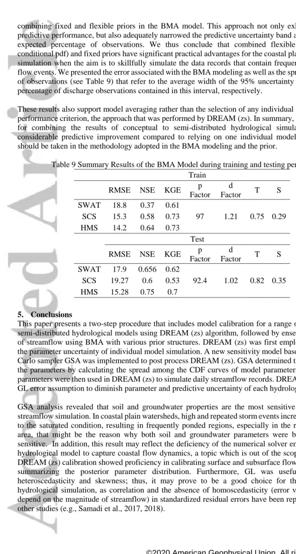
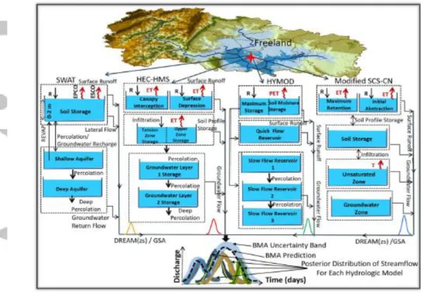
A linkage between multiple hydrological models used in this study and BMA with the various priors is illustrated in Figure 2. Briefly, the simulation of the UW2 is achieved using conceptual to semi-distributed rainfall-runoff models. Due to the computational burden of the BMA code, this study used two steps to combine the results of hydrological models. First, the outputs of models were coupled with GSA and DREAM(zs) algorithm to assess the sensitivity and parameter uncertainty of the models. Next, the outcomes of hydrological models were fed to the BMA to combine the simulation with the most important parts of the posterior model distribution of hydrological model and improve daily streamflow prediction. A weighted posterior probability simulation was then outperformed using BMA with the most appropriate fixed and flexible priors for the watershed under study.
3. Applications to Rainfall‐Runoff Modeling 3.1. Parameter Sensitivity Analysis
In this study, SWAT and HEC-HMS models were forced by 18 parameters, while HYMOD and modified SCS-CN were calibrated using five and 14 parameters, respectively. Parameter sensitivity analysis proved that the DREAM(zs) sampling algorithm is onerous and time consuming, especially for the SWAT and HEC-HMS analyses. This is partly related to the fact that some parameters contributed more weight to simulation, making the MCMC results being more sensitive to changes of these parameters. For instance, shallow aquifer and soil properties are two key parameters that are proved to have a significant effect on the coastal plain simulation (e.g., Samadi and Meadows, 2017; Samadi et al., 2017).
Marginal distributions derived from DREAM(zs) were computed for all four hydrological models (results not shown here). Optimal parameter values, and the upper and lower bounds that define the prior uncertainty ranges of HYMOD parameters as well as sensitivity rank are given in Table 1. In HYMOD, residence time slow flow reservoir (days) that computes the groundwater parameter showed more spiked and narrower range and depicted most sensitive parameters (see Table 1) whereas parameters related to quick flow (e.g., Rq) were ranked as the most insensitive ones. Note that the marginal pdfs of the HYMOD parameters appeared approximately Gaussian except for those of bexp and
Rs, which significantly departed from a normal distribution and tended to concentrate most of the
probability mass at their upper and lower bounds (sharp response; results not shown here). Indeed, the mathematical approaches used to estimate bexp and Rs appear to be insufficient to capture appropriate
ranges for the spatial variability of the soil moisture storage as well as the residence time of groundwater flow.
Table1. HYMOD parameters, initial parameters range, their optimal values driven by DREAM(zs), and the parameters sensitivity rank.
Parameter Number
Parameter Description K-S Value
Minimum Maximum Sensitivity Rank Optimum Value 1 Cmax maximum storage in watershed (mm) 0.32 1.00 500 4 213.07 2 bexp spatial variability of soil moisture storage 0.45 0.10 2.00 2 1.99 3 Alpha distribution factor between two reservoirs 0.36 0.10 0.99 3 0.17 4 Rs residence time slow flow reservoir (days) 0.66 0 0.10 1 0 5 Rq residence time quick flow reservoir (days) 0.25 0.1 0.99 5 0.1958
The HEC-HMS model results indicate that the range of maximum infiltration was considerably narrowed by DREAM(zs), whilst other parameters such as groundwater, maximum percolation, and threshold to peak flow occupied a relatively large region interior to the uniform prior distribution. These ranges were not further narrowed by DREAM(zs) even when the number of iterations were increased. Further, the ranges of the GW2 routing coefficient, storage capacity and GW1 storage capacity narrowed significantly by the MCMC algorithm indicating the sensitivity associated with these parameters in the model (see Table 2). HEC-HMS showed low sensitivity when the tension capacity was lower than storage capacity; thus, a multiplier-value was used for the storage capacity. What should be noted here is that the degree of sensitivity of infiltration rate, storage and groundwater routing showed more fluctuations that could be decreased if groundwater/shallow aquifer properties were formulated appropriately by the HEC-HMS. This is because there is a strong interaction among shallow aquifer properties, overland flow and channel routing parameters in the coastal plain drainage system as recently shown by Samadi and Meadows (2017). This interaction may affect the runoff amount and
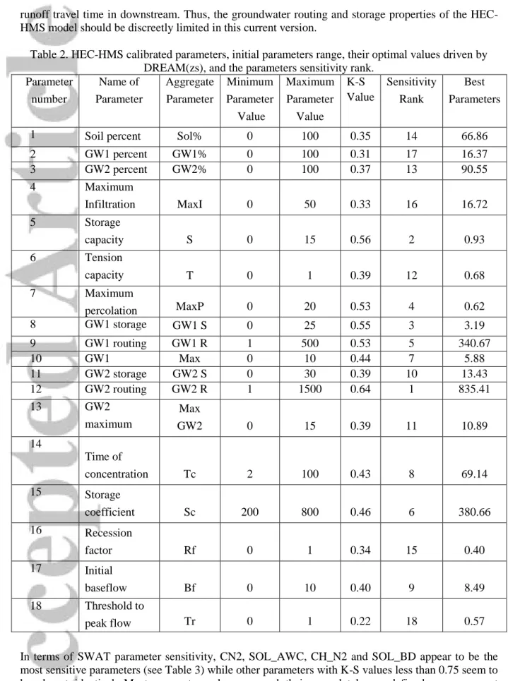
runoff travel time in downstream. Thus, the groundwater routing and storage properties of the HEC-HMS model should be discreetly limited in this current version.
Table 2. HEC-HMS calibrated parameters, initial parameters range, their optimal values driven by DREAM(zs), and the parameters sensitivity rank.
Parameter number Name of Parameter Aggregate Parameter Minimum Parameter Value Maximum Parameter Value K-S Value Sensitivity Rank Best Parameters
1 Soil percent Sol% 0 100 0.35 14 66.86
2 GW1 percent GW1% 0 100 0.31 17 16.37 3 GW2 percent GW2% 0 100 0.37 13 90.55 4 Maximum Infiltration MaxI 0 50 0.33 16 16.72 5 Storage capacity S 0 15 0.56 2 0.93 6 Tension capacity (multiplier) T 0 1 0.39 12 0.68 7 Maximum percolation MaxP 0 20 0.53 4 0.62 8 GW1 storage capacity GW1 S 0 25 0.55 3 3.19 9 GW1 routing coefficient GW1 R 1 500 0.53 5 340.67 10 GW1 maximum percolation Max GW1 0 10 0.44 7 5.88 11 GW2 storage capacity GW2 S 0 30 0.39 10 13.43 12 GW2 routing coefficient GW2 R 1 1500 0.64 1 835.41 13 GW2 maximum percolation Max GW2 0 15 0.39 11 10.89 14 Time of concentration Tc 2 100 0.43 8 69.14 15 Storage coefficient Sc 200 800 0.46 6 380.66 16 Recession factor Rf 0 1 0.34 15 0.40 17 Initial baseflow Bf 0 10 0.40 9 8.49 18 Threshold to peak flow Tr 0 1 0.22 18 0.57
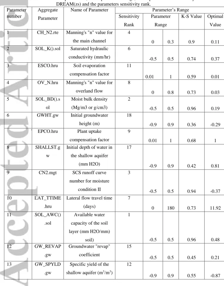
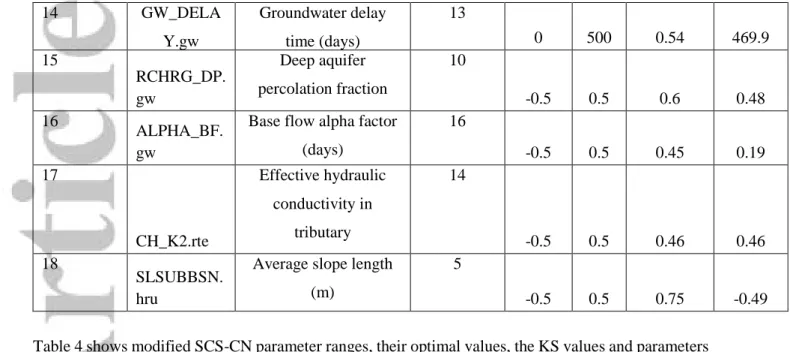
In terms of SWAT parameter sensitivity, CN2, SOL_AWC, CH_N2 and SOL_BD appear to be the most sensitive parameters (see Table 3) while other parameters with K-S values less than 0.75 seem to be almost identical. Most parameter values covered their completely pre-defined ranges except SOL_AWC and SOL_K. The ranges of these parameters are narrower than their pre-defined scopes suggesting high sensitivity of SWAT groundwater parameters. Further, some of SWAT parameters occupied a relatively small region interior to the uniform prior distributions of the individual dimensions (results not shown). This reveals that the observed streamflow data contains sufficient information to
estimate these parameters. This is further confirmed with relatively small parameter ranges as shown in Table 3.
Table 3. SWAT calibrated parameters, initial parameters range, their optimal values driven by DREAM(zs) and the parameters sensitivity rank.
Parameter number
Aggregate Parameter
Name of Parameter Parameter’s Range
Sensitivity Rank Parameter Range K-S Value Optimal Value 1 CH_N2.rte Manning's "n" value for
the main channel
4
0 0.3 0.9 0.11
2 SOL_K().sol Saturated hydraulic
conductivity (mm/hr)
6
-0.5 0.5 0.74 0.37
3 ESCO.hru Soil evaporation
compensation factor
11
0.01 1 0.59 0.01
4 OV_N.hru Manning's "n" value for overland flow
8
0 0.8 0.73 0.03
5 SOL_BD().s
ol
Moist bulk density (Mg/m3 or g/cm3) 2 -0.5 0.5 0.96 0.19 6 GWHT.gw Initial groundwater height (m) 18 -0.9 0.9 0.36 -0.29
7 EPCO.hru Plant uptake
compensation factor
9
0.01 1 0.68 1
8 SHALLST.g
w
Initial depth of water in the shallow aquifer
(mm H2O)
17
-0.9 0.9 0.42 0.81
9 CN2.mgt SCS runoff curve
number for moisture condition II
3
-0.5 0.5 0.94 -0.37
10 LAT_TTIME
.hru
Lateral flow travel time (days) 7 0 180 0.73 11.92 11 SOL_AWC() .sol Available water capacity of the soil layer (mm H2O/mm) soil) 1 -0.5 0.5 0.96 0.48 12 GW_REVAP .gw Groundwater "revap" coefficient 15 -0.5 0.5 0.45 0.21 13 GW_SPYLD .gw
Specific yield of the shallow aquifer (m3/m3)
12
14 GW_DELA Y.gw Groundwater delay time (days) 13 0 500 0.54 469.9 15 RCHRG_DP. gw Deep aquifer percolation fraction 10 -0.5 0.5 0.6 0.48 16 ALPHA_BF. gw
Base flow alpha factor (days) 16 -0.5 0.5 0.45 0.19 17 CH_K2.rte Effective hydraulic conductivity in tributary 14 -0.5 0.5 0.46 0.46 18 SLSUBBSN. hru
Average slope length (m)
5
-0.5 0.5 0.75 -0.49
Table 4 shows modified SCS-CN parameter ranges, their optimal values, the KS values and parameters sensitivity rank. As expected, subsoil drainage coefficient and coefficient of transpiration from soil zone are ranked as the most sensitive parameters. Like SWAT, modified SCS-CN showed more sensitivity to curve number. Further, this model showed more sensitivity to hydrogeological properties (e.g., subsoil permeability) and surface energy balance. It appears C1 depends on the available soil water in
the topsoil layer. PNAC is another sensitive parameter that indicates inadequate atmospheric evaporation capability in the model.
Table 4. Modified SCS-CN calibrated parameters, initial parameters range, their optimal values driven by DREAM(zs) and the parameters sensitivity rank.
3.2.DREAM(zs) Predictive Uncertainty
Once the posterior distribution of the model parameters is determined, the predictive uncertainty of daily discharge simulation for each hydrological model was computed by propagating the different samples of the posterior distribution at the 95% confidence interval. Table 5 compares the results of DREAM(zs) simulation for different hydrological models. Based on several performance criteria, SWAT well calibrated streamflow records compared to the rest of models. This would imply that the GL function, used as an objective function in DREAM(zs) to remove heteroscedasticity and autocorrelation, was particularly successful for a semi-distributed hydrological model calibration. The modified SCS-CN model and HEC-HMS are posed in the next ranks. The HYMOD model showed the weakest performance, which may be because of its simplicity and lumped concept.
Figures 3, 4, 5, and 6 show diagnostic plots of the residuals (i.e. difference between observed and simulated streamflow) derived from the GL likelihood function. In most cases, the heteroscedasticity has been removed by the GL function and the residuals are not sensitive to the magnitude of streamflow. Figures 3(b), 4(b), 5(b), and 6(b) clearly show that the double exponential (heavy-tailed) distribution used by the error model is suitable and consistent with the pdf of the residuals. This would reveal that
Parameter number Name of Parameter Minimum Parameter Value Sensitivity Rank K-S Value Maximu m Paramete r Value Aggregate Parameter Optima l Value 1 Curve number 70 3 0.82 90 CN0 88.76 2 Coefficient of the initial abstraction 0.01 4 0.69 0.7 λ1 0.01 3 exponent of the initial abstraction 0.01 14 0.20 10 Α 7.40 4 coefficient of antecedent moisture 0.1 6 0.56 10 Β 8.84 5 storage coefficient 0.001 7 0.52 20 K 14.65 6 coefficient of transpiration from soil zone 0.01 2 0.93 1 C1 0.01 7 subsoil drainage coefficient 0.001 1 0.94 1 C2 0.0013 8 maximum potential water retention (mm) 300 12 0.24 5000 S abs 304.53 9 wilting point of the soil (mm) 5 13 0.23 250 θw 246.03 10 Fraction of field capacity of the soil (mm) 0.001 8 0.46 0.55 θf 0.51 11 unsaturated soil zone runoff coefficient 0.01 10 0.29 1 C3 0.106 12 exponent of groundwater zone 0.01 9 0.32 2 E 0.011 13 groundwater zone
runoff coefficient 0.005 11 0.27 1 BCOEF 0.08
14 Pan coefficient
MCMC Bayesian algorithm applied in this study is promising for relaxing the residual error assumption of the upper Waccamaw watershed.
Temporal dependence of the residuals is illustrated in Figures 3(c), 4(c), 5(c), and 6(c), which indicate that the residuals still exhibit substantial dependence at higher lag autocorrelations. Although autocorrelation of the residuals has been substantially reduced by DREAM(zs), the challenge of omitting temporal correlation in the coastal plain simulation is understandable. DREAM(zs) was particularly successful in eliminating temporal dependencies in SWAT and modified SCS-CN simulation. HEC-HMS and modified SCS-CN predictive uncertainty seems to be similar, although the latter one provided a wider band. HYMOD, on the other hand, converged to a very different posterior pdf revealing less capability of this model in simulating flow dynamics across a coastal plain environmental system. However, DREAM(zs) was somewhat successful in removing correlation in the HYMOD model.
Overall, the total predictive uncertainty bound seems reasonably accurate for SWAT and HEC-HMS (see Figures 7, 8, 9, and 10). These two models mimicked the observed data quite well, reproducing most minor and major flow events. However, closer inspection of the calibration results indicates that DREAM(zs) was not quite successful in calibrating the modified SCS-CN model. Further, HYMOD results revealed that, although error assumptions are fulfilled, the predictive uncertainty band is too large and meaningless. This indicates that this model is less capable of simulating coastal rainfall-runoff processes. On the other hand, the inconsistency in simulation may also arise due to uncertainty in input data when repeated rainfall events occur in the coastal plain (e.g. Samadi et al., 2018).
The assumption of a double exponential prior distribution, as explained above, relatively well approximated the conditional pdf of SWAT, HEC-HMS and the modified SCS-CN model. Daily streamflow data of the coastal drainage system are naturally bounded by fat- to highly skewed-tailed distributions which is difficult to justify according to the outcomes of one specific prior distribution. This inspired the authors to employ BMA with a hierarchy of prior formulations to marginally combine the simulation on the most important parts of the posterior probability distribution of each potential hydrological model explained in next section.
Table 5. Performance criteria for different hydrological models. Model
Total Uncertainty Parameter Uncertainty Best
Simulation
P-Factor
d-Factor T S P-Factor d-Factor T S KGE NSE RMSE
HEC-HMS 93.43 2.07 0.61 0.18 5.47 0.08 9.11 7.15 0.74 0.72 11.98 HYMOD 93.97 2.59 0.60 0.18 8.39 0.12 12.89 10.13 0.70 0.57 15.05 SWAT 75.91 2.28 0.59 0.17 7.48 0.14 4.43 3.40 0.73 0.66 13.37 Modified SCS-CN 93.03 2.43 0.56 0.16 11.54 0.11 5.53 4.26 0.72 0.61 14.36 4. BMA Computation
The outcomes of four hydrological models were coupled with Bayesian model averaging using a variety of prior structures. This study included fixed to flexible model priors and examined the possibility of subjective inference using prior inclusion probabilities according to the user’s belief. Two efficient MCMC samplers (i.e. BD and RJMCMC) were then applied to create a weighted posterior probability distribution from BMA exercise that sorted through the model space. Below is a discussion of the results of BMA simulation for different prior structures.
4.1. Fixed Priors
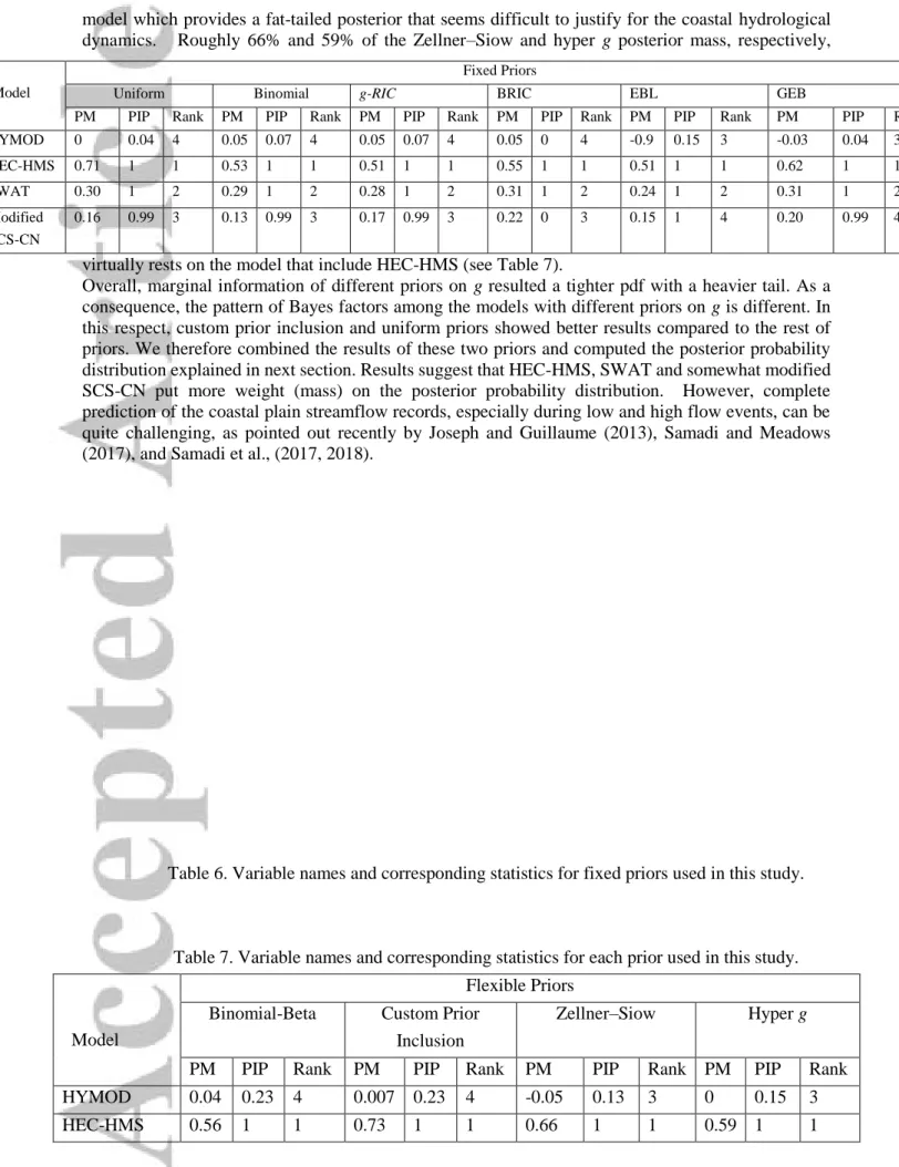
A uniform prior with the unit information prior on Zellner's g was first applied to compute the expected prior parameter size. The variable names and corresponding statistics are shown in Table 6. Posterior mean (PM) displays the coefficients averaged over all models. Posterior inclusion probabilities (PIP)
or shrinkage factor represents the sum of the posterior model probability for all models wherein a covariate (a modeled streamflow) was included. In other words, PIP displays the importance of the various hydrological models in explaining daily streamflow data. Interestingly, the majority of the posterior mass virtually rests on models that include HEC-HMS, SWAT, and modified SCS-CN. In contrast, HYMOD has the lowest PIP (i.e. 4%), indicating that HYMOD does not seem to matter much, implying an inability of a simple lumped model in simulating coastal observational records.
Accordingly, the rank of models (see Table 6) that are sorted by PIP reveals that HEC-HMS and SWAT were successful in simultaneously describing observations in terms of magnitude. The posterior expected model size (i.e., the average number of included regressors, which ranges from 1 to 5) using the uniform prior was 3.04, which is the sum of PIPs. The uniform model prior puts more mass on intermediate model sizes (e.g. k/23with 31% probability); therefore, it is important to consider
other popular priors that allow more freedom in choosing model size and other factors. It is interesting to note that the uniform prior better calibrates the shrinkage factor (or PIP) by avoiding overfitting. As the shrinkage factor increases, the model tends to yield a tighter posterior.
Next, we used a Binomial model prior to place a common and fixed inclusion probability on each hydrological model. The model included a prior model size of 2.5 (i.e.
k
/
2
2
.
5
) which tilted the prior distribution toward smaller model sizes. Simulating BMA using the Binomial prior with model size of 2.5 yielded a posterior model size of 3.07, near that of the uniform prior. As a result, the PIP of each rainfall-runoff model is the same as uniform prior. Although the PIP of HYMOD improved slightly, the rank of the hydrological models is similar to when using the uniform prior (see Table 6).In addition, BMA calibration using g-RIC, BRIC, EBL, and GEB priors were computed and the results presented in Table 6. Among these priors, EBL provided the most discouraging results, indicating marginal likelihood evaluation using a Laplace approximation was less appropriate for integrating the posteriors. Overall, these results indicate that the BMA model concentrated posterior mass tightly on HEC-HMS and somewhat SWAT whereas modified SCS-CN model resulted less model mass concentration. HYMOD was the least capable model, and thus BMA avoided including this model for summarizing the posterior mass.
4.2. Flexible Priors
In view of the pervasive impact of HEC-HMS and SWAT models on posterior model distribution, one might wonder whether their importance would still remain robust to a greatly unfair prior. In perusing this, we specified our own model priors (custom prior inclusion) and offered a possibility of subjective inference by setting prior inclusion probabilities according to the user belief. We defined a low prior inclusion probability (i.e.
0
.
01
) for the HEC-HMS and SWAT simulations whilst setting a standard prior inclusion probability of
0.5for the rest of the hydrological models. Results indicated that HEC-HMS and SWAT still retain their shrinkage factors near 100%. Posterior model size, on the other hand, increased to 3.2 while HYMOD obtained a larger PIP (0.16). The modified SCS-CN model also retained its PIP of 99%. The coefficients averaged over all models improved slightly for HYMOD where it remained similar for the rest of models.The Binomial-Beta prior was the second prior that was implemented for the BMA calibration. Since the fixed common
in the Binomial prior (explained above) centers the mass of its distribution near the prior model size, this may increase prior uncertainty about model size. Thus, Ley and Steel (2009) proposed to include a hyperprior on the inclusion probability of
that effectively draws from a Beta distribution. In pursuing this, the Binomial-Beta prior put a completely flat prior on an expected model size of each hydrological model. Consequently, the posterior model size resulted in a value of 3.32. In terms of coefficient and posterior model size distribution, the results are similar to Binomial model priors, although the latter approach involved a tighter model prior. The use of the Binomial-Beta framework supports the results found in aforementioned prior calibrations that 100% of all posterior mass virtually rests on model