Simple Monetary-Fiscal Targeting Rules

C

ENTRE FOR

D

YNAMIC

M

ACROECONOMIC

A

NALYSIS

W

ORKING

P

APER

S

ERIES

*_{Acknowledgements: I should like to thank Sean Holly, Kaushik Mitra and Charles Nolan for useful}

comments and the Centre for Dynamic Macroeconomic Analysis at the University of St Andrews for generous research funding.

†_{Centre for Dynamic Macroeconomic Analysis, School of Economics and Finance, Castlecliffe, The}

Scores, St Andrews, Fife KY16 9AL, Scotland, UK. Tel +44 (0) 1334 462 445. E-mail: [email protected].

CASTLECLIFFE, SCHOOL OFECONOMICS& FINANCE, UNIVERSITY OFSTANDREWS, KY16 9AL TEL: +44 (0)1334 462445 FAX: +44 (0)1334 462444 EMAIL: [email protected]

CDMA08/01

Simple Monetary-Fiscal Targeting Rules

*

Michal Horvath

University of St Andrews

J

2008

A

We analyze the characteristics of optimal dynamics in an economy in which neither prices nor wages adjust instantaneously and lump-sum taxes are unavailable as a source of government finance. We then propose that monetary and fiscal policy should be coordinated to satisfy a pair of simple specific targeting rules, a rule for (wage) inflation and a relationship that links the growth of real wages to past price and wage developments, and output gap dynamics. We show that such simple rule-based conduct of policy can do remarkably well in replicating the dynamics of the economy under optimal policy following a given shock.

JEL Classification: E52, E61, E63.

Keywords:Optimal Monetary and Fiscal Policy, Timeless Perspective, Nominal Rigidity, Simple Targeting Rules.

1. Introduction

In this paper, we propose simple ‘speci…c targeting rules’in the spirit of Svensson (2002, 2003) to characterize ‘desirable’policy in a New Keynesian economy with staggered wage and price contracts, and endogenous tax dynamics. In our complex analytical framework, which is an extension of Erceg et al. (2000) and Benigno and Woodford (2003, 2004), it is not possible to characterize optimal policy using

simple analytical solutions. Our approach of looking at joint monetary-…scal

targeting rules represents an innovative way of approximating optimal policy that allows us to obtain an excellent match with the optimal dynamics of the economy following shocks.

Our work is also related to Schmitt-Grohé and Uribe (2005) and Chugh (2006) who studied jointly optimal monetary-…scal strategies in frameworks involving costly price and wage adjustment. By doing so, they extended upon a stream of literature on monetary and …scal policy that begins with Lucas and Stokey’s (1983) ‡exible-price framework with complete asset markets and has gradually evolved over time to include asset market imperfections (Aiyagari et al., 2002) and price stickiness (Benigno and Woodford, 2003, Schmitt-Grohé and Uribe, 2004a and Siu, 2004).

Our analysis is distinct in the class of papers with price and wage rigidity in two important aspects. First, it follows the linear-quadratic approach of Erceg et al. (2000) and Benigno and Woodford (2004) to analyze jointly optimal monetary-…scal strategies. This allows us to characterize optimal policy using a quadratic objective function, which is appealing from a practical point of view, and to directly compare its properties with the policy objectives derived in a similar way in the simpler economies of Erceg et al. (2000) and Benigno and Woodford (2004). Second, we depart from the conventional approach, used among others in

Erceg et al. (2000) and Schmitt-Grohé and Uribe (2004b, 2005), of looking for simple rules for policy instruments to approximate optimal policy. We propose a simple characterization of policy as an approximation to the optimal policy at a higher level of generality, as discussed in Svensson (2002, 2003) and Svensson and Woodford (2005). We concentrate on ‘speci…c targeting rules’. These rules o¤er a simple joint policy target for monetary and …scal policy makers. We show that well-speci…ed simple speci…c targeting rules can guide policy very well so that when combined with the structural model, the resulting dynamics of the economy is a close approximation of the dynamics under optimal policy following a given shock. Such simple characterization of policy has thus the potential to outperform simple (ad hoc) instrument rules. In other words, conduct of policy based on conventionally considered simple instrument rules would lead to excessive welfare losses some of which can be eliminated if policy is characterized, as we propose, at a higher level of generality. We demonstrate this point by deriving ‘expectations-based reaction functions’(Evans and Honkapohja, 2006) consistent with the simple targeting rules and showing that they are much more complex than the conventionally considered instrument rules. At the same time, from a practical point of view, characterization of policy via the targeting rules proposed here is no less veri…able than the conduct of policy based on commitment to

instrument rules. Speci…c targeting rules are also equally easy to build into

macroeconomic decision frameworks. As spelled out in detail in Svensson (2002, 2003), characterizing policy using targets rather than simple rules for instruments is also more consistent with the use of judgement in policy making. On the other hand, the quality of approximation provided by speci…c targeting rules is prone to be a¤ected by the dynamic structure of the economy modelled. Nevertheless, and especially given the reluctance of policy makers to commit themselves to an explicit instrument rule, and the popularity of target-based conduct of monetary

policy, we consider speci…c targeting rules an attractive and policy-relevant way of characterizing ‘good’policy.

In our sticky-price, sticky-wage framework, we …nd that the central government’s policy objective includes a wage in‡ation volatility term in addition to the objective of stabilizing price in‡ation and output gap volatility. Hence, this result from Erceg et al. (2000) and Benigno and Woodford (2004) carries over

to a situation when monetary policy has …scal implications too.1 _{We also …nd}

that the relative weights in the policy objective are little changed compared with Benigno and Woodford (2004). As expected, optimal nominal wage volatility falls dramatically with wage-stickiness and this causes real wages to be much more stable compared with the sticky-price but ‡exible-wage model of Benigno and Woodford (2003), for instance. The presence of nominal wage stickiness also introduces endogenous persistence into the dynamics of the model. In contrast to the ‡exible-wage Benigno and Woodford (2003) economy, our endogenous variables converge to their (new) steady state levels only gradually, even if the disturbance that initially causes the economy to abandon its steady state is purely transitory. Non-stationarity in the dynamics of public debt, tax rate and the output gap carries over from Benigno and Woodford (2003) as the optimal solution to an economy where wage stickiness is present in addition to price stickiness. We …nd some support for the claim that price stickiness is the single most important factor justifying price stability as the principal goal of monetary policy (Schmitt-Grohé and Uribe, 2005). We also show that it is enough for one of the markets to be imperfectly ‡exible to make the policy of strict price- and wage-level targeting undesirable.

1_{Adding further frictions to the model such as rule-of-thumb behaviour, various indexation}

mechanisms or habit persistence would be likely to a¤ect the nature of the policy objective, as in Amato and Laubach (2003), for instance. Our purpose here is to examine the e¤ect of the absence of lump-sum taxation on the policy objective and optimal dynamics in isolation.

We then propose that the branches of central government authority operating in our sticky-price, sticky-wage economic framework should coordinate their e¤orts to gradually stabilize nominal wage growth and also make sure that a simple relationship linking the growth in the real wage rate to past price and wage in‡ation and the dynamics of the output gap is satis…ed. We rank alternative policies in the family of policies given by these simple targeting rules. Benigno and Woodford (2006b) discuss in great detail the issues associated with ranking suboptimal rules in frameworks such as ours. The method for ranking suboptimal simple rules proposed in Benigno and Woodford (2006b), which entails separating the trend and the cyclical components of di¤erence-stationary series (output gap) and ranking of policies implying the same trend component using a similar decomposition of welfare, cannot be applied in our case, since the policies we wish to examine do not converge to the same long-run outcome (i.e. have di¤erent trend components). Instead, we identify the best policy in our class using a simple grid search over a (constrained) range of parameters to obtain the parameter values that would calibrate our rules so that the implied impulse response functions for the variables in the policy objective come closest to those describing the behaviour of the optimal economy following the same shock. A similar criterion was shown to be a good alternative to analyses based directly on utility-based measures of welfare in Schmitt-Grohé and Uribe (2005).

The structure of the paper is as follows. Section 2 presents the microeconomic foundations of our sticky-price, sticky-wage model. In Section 3, we outline the corresponding macroeconomic model and discuss the policy makers’ objective.

We also examine the feasibility of some simple policy strategies. In Section

4, we derive the ‘timelessly optimal’ plan. In Section 5, we propose a pair

of simple targeting rules to approximate optimal policy and analyze how the economy performs relative to the optimal economy under such a characterization

of policy. Since the steps involved in deriving the model of the macroeconomy and the approximate Ramsey problem directly follow from Benigno and Woodford (2003, 2004), the Appendix to this paper only lists some key relationships between parameters and variables. The derivations of the structural relationships and of the policy objective are available upon request from the author.

2. The microeconomic foundations

Our model economy is inhabited by an in…nite number of identical households of measure one. The representative household derives positive utility from total

consumptionC of di¤erentiated goods and incurs disutility from supplying labour

h, which is captured by the utility function

Ut =Et 1 X T=t T t uT; (2.1) ut =U Ct;Gbt Z 1 0 (ht(j))dj: (2.2)

0 < < 1 is the subjective discount rate. The household supplies

industry-speci…c labour toj industries. As explained in Woodford (2003, Chapter 3), this

is equivalent to assuming that each household is employed in one type of industry only and the existence of perfect capital markets to enable risk-sharing across industries. We assume the following speci…c functional forms

U Ct;Gbt = C_t1 e 1 1 _e 1; (2.3) (ht(j)) = ht(j)1+!w 1 +!w ; (2.4)

where _e and !w are constants. In the utility function, Gbt stands for a shock to

Consumption of individual goods is aggregated into a total consumption index using a standard Dixit-Stiglitz (1977) aggregator

Ct = Z 1 0 ct(i) "p 1 "p _di "p "p 1 ; (2.5)

in which"p is a constant and represents the elasticity of substitution across goods

in the goods market. Minimization of an expenditure function subject to (2.5)

yields an expression for the optimal consumption of good i. A standard income

identity then implies the demand function

yt(i) =Yt

pt(i)

Pt "p

: (2.6)

The corresponding price index is written as

Pt= Z 1 0 pt(i) 1 "p di 1 1 "p : (2.7)

We introduce imperfect competition into the labour market in a similar way. We assume the existence of a continuum of monopolistically competitive households, supplying di¤erentiated labour to the production sector. The total

quantity of labour used in the production of good i is an aggregate of di¤erent

types of labour indexedj.

Ht(i) = Z 1 0 ht(j) "w 1 "w dj "w "w 1 ; (2.8)

in which "w is the elasticity of substitution in the labour market. It is assumed

that there exists an employment agency that bundles together di¤erent types of

labour needed in the production of a good i exactly in the same way as the …rm

producing that good would want it. Cost minimization by wage-taking …rms

subject to (2.8) yields the demand for labour of typej

ht(j) =Ht

wt(j)

Wt "w

and the nominal wage index Wt= Z 1 0 wt(j)1 "wdj 1 1 "w : (2.10)

Note that aggregate labour supply in the economy can then be expressed as

Ht =

R1

0 Ht(i)di. Combining this with the production function and (2.6) yields

the expression for total labour supply in the economy

Ht=Yt p;t; (2.11)

where p;t refers to price dispersion and is given by

p;t = Z 1 0 pt(i) Pt "p di: (2.12)

The total disutility from supplying labour can then be expressed as

Z 1 0 (ht(j))dj = 1 1 +!w Y (1+!w) t 1+!w p;t w;t; (2.13)

where w;t stands for wage dispersion and is given by

w;t = Z 1 0 wt(j) Wt "w(1+!w) dj: (2.14)

2.1. The wage-setting decision

Each household maximizes the di¤erence between the utility derived from wage income and the disutility from labour supply

Uc Ct;Gbt

Pt

(1 w;t)wt(j)ht(wt(j)) (ht(wt(j))): (2.15)

Moreover, it does so in a forward-looking way, evaluating an expected stream of net utility gains. As in Erceg et al. (2000), we assume a wage setting mechanism

of not being able to adjust wages in any period. The intertemporal …rst-order condition can then be written as

Et 1 X T=t ( T t w Qt;THt wT (j) WT "w 2 4(1 w;T) wH !w T PT WT 1 Uc CT;GbT wT (j) WT "w!w 1 3 5 9 = ;= 0

in which w is the rate of distortive tax on wage income. Under the baseline Calvo

framework,wT (j) =wt(j) for allT. This implies that …rms will charge the price

chosen in period t, if they do not receive a signal that they can adjust their prices

in period T (with probability T t

w ). Qt;T is a standard stochastic asset pricing

kernel that can be derived from a simple household utility maximization problem subject to a ‡ow budget constraint equating wage and dividend income together

with asset returns to consumption and change in assets. w is the wage markup

and is given by

w =

"w

"w 1

: (2.16)

In a symmetric equilibrium, suppliers of labour who change their prices in periodt

set a common wage so thatwt(j) =wt. We can now solve the …rst-order condition

from the wage-setting problem for wage dispersion

w_t Wt = 2 6 6 4 Et 1 P T=t ( _w )T t _wY (1+!w) T 1+!w p;T WT Wt "w(1+!w) Et 1 P T=t ( _w )T tUc CT;GbT W_PTTYT p;T (1 w;t) W_WT_t "w 1 3 7 7 5 1 1+"w !w = Kw;t Fw;t 1 1+"w !w : (2.17)

The assumption of baseline Calvo-pricing implies the following law of motion for the wage index

Wt = (1 w)w 1 "w t + wW 1 "w t 1 1 1 "w _{: (2.18)}

Combining (2.17) and (2.18) gives us an implicit de…nition of the nominal wage growth " 1 _w "w 1 w;t 1 _w #1+"w !w "w 1 = Fw;t Kw;t ; (2.19) where w;t = _WWt

t 1. It is now also easy to show that

w;t= w "w(1+!w) w;t w;t 1+ (1 w) " 1 _w "w 1 w;t 1 _w # "w(1+!w) 1 "w : (2.20)

2.2. The price-setting decision

Firms maximize a future stream of pro…ts with wages being the only cost item in

their balance sheets. The nominal pro…t of …rmi is written as

zt(i) = pt(i)yt(i) WtHt(i): (2.21)

Here, we also assume a baseline Calvo price-setting mechanism with _p being

the probability of having to leave prices unchanged in a given period. The

representative …rm is then choosing the optimal price, taking the wage index as given, and the intertemporal …rst-order condition is written as

Et 1 X T=t T t p Qt;TYT pt(i) PT "p" 1 _pWT PT Y_T 1 pt(i) PT "p( 1) 1# = 0 (2.22)

We can de…ne !p = 1 and as before, the markup is given by

p =

"p

"p 1

: (2.23)

Forpt(i) =pt; we obtain a closed-form solution

p_t PT = Kp;t Fp;t 1 1+"p!p (2.24)

with Kp;t=Et 1 X T=t p T t Uc CT;GbT p WT PT Y_T PT Pt "p(1+!p) ; (2.25) Fp;t=Et 1 X T=t p T t Uc CT;GbT YT PT Pt "p 1 : (2.26)

The price index evolves according to

Pt= h 1 _p p 1 "p t + pP 1 "p t 1 i 1 1 "p ; (2.27)

which together with (2.24) implies the following implicit de…nition of price

in‡ation p;t= _PP_tt₁ " 1 _p "p 1 p;t 1 _p #1+"p!p "p 1 = Fp;t Kp;t : (2.28)

The law of motion for price dispersion as de…ned in (2.12) is

p;t = p "p(1+!p) p;t p;t 1+ 1 p " 1 _p "p 1 p;t 1 _p # "p(1+!p) 1 "p : (2.29) 2.3. Central government

Monetary and …scal authorities, the two branches of the central government, coordinate their actions to ensure that social welfare given by (2.1) is maximized. The government raises revenues via distortive taxes on wage income to …nance

exogenous government spendingG. It issues one-period nominal bonds to bridge

the gap between taxation and spending. The government therefore faces the ‡ow budget constraint

Bt= (1 +it 1)Bt 1 Pt t; (2.30)

where B denotes the volume of one-period nominal bonds issued by the …scal

rate. Aggregate tax receipts are given by

Tt = w;twR;tYt p;t: (2.31)

This constraint can be rewritten as

bt

(1 +it)

= bt 1

p;t

t: (2.32)

The nonlinear Ramsey problem is then to maximize (2.1) subject to the …rst-order conditions from the optimization problems of the consumers and …rms, the …scal solvency requirement, the dynamics of the price and wage dispersion, and the relevant initial and terminal conditions, alongside appropriate (initial) commitments that ensure time-consistency of the solution in the absence of

full commitment.2 _{This problem would yield a system of nonlinear …rst-order}

conditions. One can then solve for optimal dynamics using the nonlinear

model or linearize the nonlinear system to obtain an approximate solution. An equivalent way of solving for the approximate optimal plan is to formulate a linear-quadratic approximate policy problem (see Benigno and Woodford, 2003, 2006b for a thorough treatment of a general class of problems which includes the one considered here). In frameworks where stabilization policy has signi…cant …rst-order welfare e¤ects, the construction of a correct second-…rst-order-accurate welfare objective requires a second-order approximation to the structural equations. In the next section, we present the structural elements of the approximate problem.

3. The macroeconomic model

We …nd that the absence of lump-sum taxation as a source of government …nance does not change the nature of policy makers’ preferences as expressed by a

2_{Such formulation of the policy problem is now standard and is not presented here to}

quadratic loss function. It follows from our setup that the monetary and …scal branches of central government should conduct monetary and …scal policy to minimize the quadratic loss function

Lt=Et 1 X T=t T t 1 2qyy 2 T + 1 2q p 2 p;T + 1 2q w 2 w;T : (3.1)

As in Benigno and Woodford (2003, 2004), yt is the welfare-relevant output gap

de…ned as the di¤erence between the actual and the target deviation in outputYb_t .

The target deviation follows from the approximation to individual utility, hence it is determined by preferences and is independent of policy (see the Appendix).

p;t stands for price in‡ation and w;t stands for nominal wage growth or wage

in‡ation. If appropriate initial commitments are satis…ed, this objective represents a second-order-accurate welfare-ranking criterion, while the rest of the model is speci…ed with only …rst-order accuracy. The functional form is thus the same as in Erceg et al. (2000) and Benigno and Woodford (2004). The objective contains a wage-in‡ation-stabilization term, which is absent in ‡exible-wage frameworks such as Benigno and Woodford (2003). As one would expect though, the coe¢ cients as well as the target deviation in output will, in general, be di¤erent given the di¤erent structural setup caused by the unavailability of lump-sum taxation.

For common parameter values, the coe¢ cients in the policy objective will be positive, implying that the function is convex and the optimal solution that we obtain represents a minimum from the perspective of welfare losses.

The setup presented in the previous section also implies the following structural relationships for the economy. The supply side is characterized by

p;t= pyt+ p wbR;t wbR;t + Et p;t+1; (3.2)

Equation (3.2) is the price aggregate supply relationship. wb_R;t is the deviation in the real wage rate from its steady state value that brings about the target deviation in output without a¤ecting the price level. Equation (3.3) is the wage

aggregate supply relationship. _bw;t is the deviation in the tax rate that aligns the

natural rate of output with its target level, as in Benigno and Woodford (2003). It is determined based on the di¤erence in the degree to which the natural and the

welfare-e¢ cient levels of output are a¤ected by the rise in government spending.3

The dynamics of real wages is given by

b

wR;t wbR;t 1 = w;t p;t: (3.4)

Chugh (2006) highlights the central importance of this identity in determining the optimal dynamics of the economy and optimal in‡ation volatility when wages are

sticky.4 _{The ‡ow government budget constraint, together with a standard Euler}

equation and a transversality condition, implies the following …scal sustainability condition bbt 1 p;t 1yt = 't+ (1 ) fyyt+f bw;t bw;t +fw wbR;t wbR;t + Et h bbt p;t+1 1yt+1 i (3.5)

'_t is again the ‘…scal stress’ term introduced in Benigno and Woodford (2003).

The coe¢ cientsfy; f ; and fw are de…ned in the Appendix. Finally, the demand

3_{Brie‡y, the natural rate of output is the level of output that would prevail in an economy}

with no nominal rigidities. See Woodford (2003) for a thorough treatment.

4_{Under staggered wage adjustment, nominal wage growth is costly in welfare terms, as it}

generates an ine¢ cient allocation of resources due to wage dispersion and hence its desired volatility will be low. Assuming that real wage dynamics is determined elsewhere in the system and is fairly stable, in‡ation varies only to deliver the desired path of real wages. This role of in‡ation, according to Chugh (2006), dominates its role of a shock absorber. Hence, he obtains low volatility of in‡ation to be optimal even when only wage adjustment is costly. This contrasts with Schmitt-Grohé and Uribe (2005) who …nd prices to be optimally volatile when wages only are in‡exible.

side of the economy is given by the ‘IS’relationship

yt=Etyt+1 bit Et p;t+1 brt ; (3.6)

in whichr_bt is the ‘e¢ cient’deviation in the interest rate that is consistent with the

target deviation in output. This equation follows from a standard Euler equation. 3.1. Some simple policy considerations

Erceg et al. (2000) have argued that the policy maker is able to achieve maximum

welfare— the Pareto optimum, as they referred to a value of zero ofLt— if prices

in either the product or labour market are perfectly ‡exible. In that case, a policy of zero in‡ation in the ‘non-‡exible’ market will be consistent with maximum welfare. Benigno and Woodford (2004), however, overturned their result showing that the presence of cost-push shocks in economies where stabilization policy has signi…cant …rst-order welfare e¤ects will prevent such policies being feasible.

In our model, there is a new element. Since the dynamics of the tax rate is endogenous, the tax rate as a policy variable can be used to counteract cost-push pressures in the economy. On the other hand, the optimal economy also has to satisfy the constraint on government …nancing. Therefore, in the context of our model, we can formulate the following proposition.

Proposition 3.1. a) Perfect stabilization of nominal wages with the aim of

attaining the Pareto optimum is a feasible policy under ‡exible prices but sticky wages if and only if

b) Similarly, it is feasible to engineer a policy of zero price in‡ation to attain the Pareto optimum under ‡exible wages but sticky prices if and only if

bbt 1+'t= 0 for all t: (3.8)

Proof a) Since prices are fully ‡exible, the price aggregate supply relationship is vertical and price in‡ation volatility carries zero weight in (3.1). Price in‡ation

p can then serve the purpose of maintaining

b

wR;t=wbR;t for all t; (3.9)

given that w;t= 0 at all times, so that withbw;t=bw;t for allt, zero output gaps

are realized for allt and the Pareto optimum is attained. However, price in‡ation

is also the only means available to satisfy the …scal solvency constraint. With no output gap and no ‘tax gap’either, (3.5) is satis…ed if and only if

bbt 1+'t= p;t for all t: (3.10)

Equations (3.4), (3.9) and (3.10) lead to (3.7). With this, all constraints are satis…ed and the zero-in‡ation, zero-output-gap Pareto optimum is feasible. Now suppose

bbt 1+'t6=wbR;t 1 wbR;t for any t. (3.11)

For the Pareto optimum to be feasible, …scal solvency and hence (3.10) has to be

satis…ed. We can thus replace the left-hand side in (3.11) with p;t. By (3.9),

which also must hold in the Pareto optimum,w_bR;t replaceswbR;t on the right-hand

side. Combining this with (3.4) leads to the contradiction p;t 6= p;t. Thus, if

(3.7) is not satis…ed in anyt, the Pareto optimum will not be attainable.

b) In the ‡exible-wage case, with a vertical wage aggregate supply relationship,

w carries zero weight in the policy objective. It can vary freely to ensure (3.9)

output gaps are realized for all t. The Pareto optimum is feasible if and only if …scal solvency is maintained. With zero output gap, zero ‘tax gap’and zero price in‡ation, (3.5) is satis…ed if and only if (3.8) holds. This is a formal presentation of the argument in Benigno and Woodford (2003).

Neither of the conditions (3.7) and (3.8) is likely to be satis…ed under general circumstances. We can therefore conclude that the presence of distortive taxes, even though a¤ecting the structure of the economy and of the argument, it does not alter the principal conclusions from Benigno and Woodford (2004). Strict price- and/or wage-level targeting remains an undesirable policy strategy in the presence of nominal rigidity. The need to satisfy the …scal solvency condition precludes the attainment of the Pareto optimum when either of the product or labour markets is ‡exible.

4. Optimal dynamics

It is well known that optimal policy in forward-looking rational expectation frameworks is in general time inconsistent and so Woodford (2003) has proposed formulating optimal policy from a timeless perspective; one should model optimal policy as the policy that would have been intended for the current period had such a policy been formulated far in the past. Such a perspective rules out the possibility of policy makers ‘exploiting’ certain initial conditions. In order to characterize this timelessly optimal policy, we need to restrict the policy choices

for period t so that the policy maker uses the same procedure to formulate policy

as in later periods. The optimal policy is then chosen so that it satis…es certain initial (self-consistent) commitments, in addition to the structural equations

of the economy, and is characterized by a time-invariant policy rule. Our

endogenous variables the knowledge of which in periodt 1would have in‡uenced the determination of the equilibrium. These commitments re‡ect the long-run optimal solution to the dynamics of the relevant endogenous variables. The policy Lagrangian is written as Jt = Et 1 X T=t T t 1 2qyy 2 T + 1 2q p 2 p;T + 1 2q w 2 w;T + _1;T p;T pyT p wbR;T wbR;T Et p;T+1 + _2;T w;T wyT w w bw;T bw;T + w wbR;T wbR;T Et w;T+1 + _3;T [w_bR;T wbR;T 1 w;T + p;T] + _4;T hbbT 1 p;T 1yT +'T (1 )fyyT (1 )f bw;T bw;T (1 )fw wbR;T wbR;T bbT + Et p;T+1+ Et 1yT+1 io + _{4;t 1 1;t 1} p;t 2;t 1 w;t+ 1 4;t 1yt (4.1)

The …rst-order conditions (withT =t) form the following dynamic system

qyyt = p 1;t+ (1 )fy+ 1 w (1 )f w w 4;t 1 4;t 1; (4.2) q p p;t= 4;t 4;t 1 1;t 1;t 1 3;t; (4.3) q w w;t= 3;t+ (1 )f w w 4;t 4;t 1 ; (4.4) 3;t = Et 3;t+1+ p 1;t+ (1 ) fw+ f w 4;t; (4.5) 4;t=Et 4;t+1: (4.6)

The optimal dynamics of the key variables can be obtained by solving a system

comprising (4.2) to (4.6) and the constraints in (4.1). Unfortunately, the

complexity of the system does not allow us to obtain closed-form solutions for the dynamics of endogenous variables, which is the main disadvantage of this

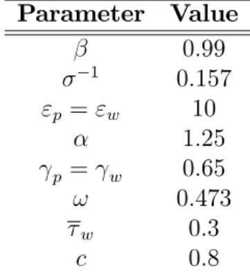
Parameter Value 0:99 1 _0:157 "p ="w 10 1:25 p = w 0:65 ! 0:473 w 0:3 c 0:8

Table 4.1: Parameter values

more complex setup. Nor can we specify optimal policy at a deeper level by deriving tractable policy targets and implied rules for monetary and …scal policy. We are therefore constrained to present the optimal dynamics in the form of numerical results. We do this below. In the next section, we shall examine simple targeting rules that do well in generating dynamics that closely matches the optimal dynamics.

4.1. Numerical analysis: Calibration and baseline results

We use the King and Watson (1998) algorithm to solve the dynamic system of …rst-order conditions and structural constraints. The parameter values used in the calibration exercise are given in Table 4.1.

The implied steady-state value of the primary budget balance as well as the values of the coe¢ cients in the policy objective are displayed in Table 4.2. We see that the relative weight of output gap stabilization remains very small. The relative weights in the objective function roughly correspond to the relative

weights obtained in the monetary policy model of Benigno and Woodford (2004).5

The system, as calibrated, satis…es the Blanchard and Kahn (1980) stability

5_{Given our calibration, the corresponding coe¢ cient values in the Benigno and Woodford}

Variable Value

Y 0:0160

qy 2:3496

q p 666:77

q w 424:29

Table 4.2: Steady-state values and coe¢ cients conditions and has a unique, stable solution, which we present below.

Based on the discussion above on the optimality of simple price- and wage-level targeting strategies, it is easy to postulate that the optimal dynamics under sticky

prices and sticky wages will not involve the pair w_bR;T;_bw;T 1

T=t and we shall

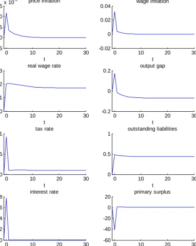
observe price and wage in‡ation and non-zero output gaps. The optimal dynamics in response to a single, serially uncorrelated positive innovation to government spending of the magnitude of one percent of steady-state output are plotted in

Figure 4.1.6 We …nd that the absence of the possibility of instantaneous real-wage

adjustment introduces endogenous persistence into the optimal dynamics of the economy. We also see that the solution includes non-stationary elements, as in the ‡exible-wage case of Benigno and Woodford (2003). While price and wage in‡ation as well as the interest rate are stationary, the output gap, real wages, the tax rate and outstanding liabilities all converge to a new equilibrium. This equilibrium is characterized by a higher tax rate and a lower output level. Hence, the non-stationarity property of the optimal dynamic solution to public debt, the tax rate and output survives in the sticky-price, sticky-wage framework as well. The near unit root property of the solution for debt is also consistent with both Schmitt-Grohé and Uribe (2005) and Chugh (2006).

6_{The value of 1 on the vertical axes denotes 1 percent deviation from the pre-shock steady}

0 10 20 30 -5 0 5 10 15x 10 -3 _{price inflation} t 0 10 20 30 -0.02 0 0.02 0.04 wage inflation t 0 10 20 30 0 0.01 0.02

0.03 real wage rate

t 0 10 20 30 -0.2 0 0.2 output gap t 0 10 20 30 0 0.5 1 tax rate t 0 10 20 30 0 0.5 1 outstanding liabilities t 0 10 20 30 0 0.02 0.04 0.06 0.08 interest rate t 0 10 20 30 -60 -40 -20 0 20 primary surplus t

4.2. Sensitivity analysis

In this section, we examine how the above reported results change when one

varies the length of contracts in both product and labour markets. Benigno

and Woodford (2003) have performed similar diagrammatic sensitivity analysis in their sticky-price, ‡exible-wage framework. They concluded that optimal (price) in‡ation volatility falls dramatically for even a small degree of price stickiness. The optimal long-run tax policy is shown to be fairly robust to the degree of price stickiness, except for the limiting case of full ‡exibility when taxes are optimally stabilized at their pre-shock steady state level in the long run. They, however, report substantial variation both in the size and the sign of the short-term response in the tax rate.

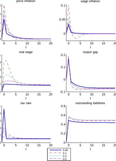
Our results for the sticky-price, sticky-wage economy are shown in Figures 4.2 and 4.3. There are several things to note about these results. First, the optimal response in the real wage rate is much smaller relative to the response in aggregate production compared with the ‡exible-wage economy at even small degrees of wage stickiness. For any length of wage contracts, we get a subdued, hump-shaped response in the real wage rate, which brings the dynamics of the model in line

with the empirical literature.7 _{Second, both price and wage in‡ation vary with the}

degree of wage stickiness but wage in‡ation is remarkably insensitive to changes in the contract length in the product market. Our analysis suggests optimal price in‡ation volatility increases considerably as one shortens the duration of price contracts while keeping wage contract duration at the baseline length. These results give some support to the conclusions of Schmitt-Grohé and Uribe

7_{Stock and Watson (1999), for instance, observe that real wages in the United States have}

displayed ‘essentially no contemporaneous comovement with the business cycle’. A similar point has been made by Christiano et al. (1997, 1999). Chadha et al. (2002) also …nd statistically insigni…cant correlation between output and real wages, though the fact that this need not hold for the entire history of UK business cycle ‡uctuations is shown in Chadha and Nolan (2000).

(2005) that price stickiness is the single most important distortion in the economy justifying price stability as the central goal of monetary policy. Third, the optimal long-run tax policy is as robust to both price and wage rigidity as it was in the case of the sticky-price economy of Benigno and Woodford (2003). However, the short-term response in the tax rate is sensitive to the degree of wage stickiness but not the length of price contracts. The tax policy here is a¤ected by the changes in the slope of the wage aggregate supply relationship and the changes in the costliness of wage in‡ation resulting from changes in the duration of wage contracts. When wages are highly rigid, the wage aggregate supply schedule is ‡at and the impact of a given tax rise on wages is only small. At the same time, nominal wage growth is very costly in welfare terms. Our results indicate that it is optimal to raise taxes sharply in the short term in response to the shock, implying that the …rst e¤ect dominates. As we approach the other extreme, the aggregate supply schedule is now steep but a given rate of wage in‡ation is less costly. Our analysis indicates that tax policy principally remains unchanged compared with the case of highly rigid wages, implying that now the second e¤ect dominates. The intermediate values of wage stickiness then imply more tax smoothing over time, characterized by a subdued initial response in taxes followed by slower adjustment to the new long-run equilibrium level. Finally, we …nd that the degree of wage or price stickiness has remarkably little e¤ect on the optimal dynamics of the output

gap both in the short run and the long run.8 _{These observations carry important}

information that we shall utilize when specifying simple targeting rules in the next section.

8_{Several of the observations here are in line with Erceg et al. (2000). Their sensitivity}

analysis implies that the variance of price in‡ation in the optimal economy is more sensitive to wage contract duration than wage in‡ation volatility to price contract duration. They also …nd that the optimal variance of the output gap is pretty stable across di¤erent combinations of price and wage stickiness.

0 5 10 15 20 0 0.05 0.1 wage inflation t 0 5 10 15 20 0 0.005 0.01 0.015 0.02 price inflation t 0 5 10 15 20 0 0.02 0.04 0.06 0.08 0.1 real wage t 0 5 10 15 20 -0.1 0 0.1 0.2 output gap t 0 5 10 15 20 0 0.2 0.4 0.6 0.8 1 tax rate t 0 5 10 15 20 0 0.2 0.4 0.6 0.8 outstanding liabilities t 0.65 0.1 0.3 0.5

0 5 10 15 20 -0.01 0 0.01 0.02 0.03 0.04 wage inflation t 0 5 10 15 20 -0.1 -0.05 0 0.05 0.1 price inflation t 0 5 10 15 20 -0.08 -0.06 -0.04 -0.02 0 0.02 0.04 real wage t 0 5 10 15 20 -0.1 -0.05 0 0.05 0.1 0.15 0.2 output gap t 0 5 10 15 20 0 0.2 0.4 0.6 0.8 1 tax rate t 0 5 10 15 20 0 0.1 0.2 0.3 0.4 0.5 outstanding liabilities t 0.65 0.1 0.3 0.5

5. Simple speci…c targeting rules

The previous section has highlighted one of the considerable weaknesses of optimal policy analysis in Ramsey-type welfare-maximizing frameworks. Even in a linear-quadratic setup that would normally yield tractable results which enable us to describe optimal paths and policy in terms of analytically simple solutions, it ultimately becomes impossible to characterize optimal policy at all levels of generality— in the sense of Svensson and Woodford (2005)— once the modelling environment becomes more complicated. One way to analyze issues in policy design is then to search for simple (linear) policy rules that can to some extent replicate the dynamics of the optimal economy and produce limited welfare losses compared with the optimal plan. In the words of Lucas (1986), such rules,

‘though certainly less e¢ cient than a monetary [and …scal] policy that reacted to real shocks in just the right way, would have welfare consequences di¤ering trivially from the optimum policy and, unlike the latter, would be easy to spell out and monitor.’

Such rules can either be ad hoc or one can employ a formal optimization procedure to determine the parameters of a ‘quasi-optimal’ rule (Currie and Levine, 1987). Erceg et al. (2000) have found simple hybrid rules that would do well compared with the fairly complicated optimized simple rule. Schmitt-Grohé and Uribe (2004b, 2005) also search for suitable rules for the interest rate and the tax rate that would approximate optimal policy.

In this section, we take a di¤erent approach. Rather than looking for ‘good’ instrument rules directly, we look for suitable characterization of policy at a higher level of generality. We identify a pair of joint policy targets which, in conjunction with the structural equations, generate dynamics similar to the dynamics of the optimal economy. Subsequently, we specify ‘expectations based reaction functions’

for monetary and …scal policy following Evans and Honkapohja (2006). The complexity of these reaction functions highlights the advantage of specifying policy at a higher level of generality, namely that it allows us to approximate a system with complex dynamic behaviour much more closely than simple instrument rules would normally do. There are thus potential gains in terms of welfare associated with the use of targeting rules as opposed to simple instrument rules.

The family of speci…c targeting rules we found useful to examine for our income-tax economy describes the policy makers’aim in terms of a rule for real wage growth as follows

b

wR;t wbR;t 1 = ( w w;t 1+ p p;t 1) y(yt yt 1) (5.1)

and a wage in‡ation targeting rule

Et w;t+1= w;t; (5.2)

with 0 < < 1. ; w; p; y and are policy parameters, where w and

p add up to one. We motivate this choice of targeting rules by the following

considerations. Benigno and Woodford (2003) show that optimal policy in a sticky-price monetary-…scal framework can be described by a pair of targeting rules (rather than a single rule, as in monetary policy models): a future (price) in‡ation target and a relationship that links current in‡ation to past in‡ation and the dynamics of the output gap. Benigno and Woodford (2004) solve for a rather more complex optimal relationship in their sticky-price, sticky-wage setup and conclude that a good approximation to optimal policy will likely entail a dynamic relationship featuring price and wage in‡ation as well as the output gap. Our targeting rule (5.1) re‡ects some of the features of their more complex

rule.9 We have also seen from the sensitivity analysis that optimal tax policy

9_{Adding further dynamic elements into (48) did not improve the results much more and}

is sensitive to wage contract duration but not to the degree of price stickiness. The same holds for nominal wage growth. It is therefore natural to think of wage in‡ation as a good candidate for an intermediate target in our

income-tax economy.10 _{Unlike in ‡exible-wage models, there is some persistence in the}

behaviour of our endogenous variables— including wage in‡ation— in the optimal economy, therefore, one should expect the targeting rule to be de…ned as a gradual adjustment process converging to a long-run target value. Hence the choice of (5.2). It follows that the choice of this second rule will likely depend on the

nature of the tax system.11

As far as rules for instruments are concerned, it is straightforward to derive the analogues of the ‘expectations based reaction function’of Evans and Honkapohja (2006) associated with our targeting rules. For monetary policy, we have

bit = brt +Et p;t+1+ 1Etyt+1 1 y p;t+ 1 y w;t + 1 y p p;t 1 + 1 y w w;t 1 1yt 1 (5.3)

The reaction function for the tax rate can be written as

bw;t = bw;t+ 1 w p p;t+ 1 w w w;t !+ 1 w yt w p (Et p;t+1 p;t); (5.4)

10_{In setups with endogenous tax dynamics, the policy regarding the tax rate plays a role in}

stabilizing prices through its impact on …rms’marginal cost. This relationship between the tax rate and wage in‡ation is also clear from the wage aggregate supply relationship (35).

11_{In our preliminary attempts, we also experimented with a price in‡ation target similar to}

the wage in‡ation target used, but it proved to be an inferior policy objective in our economy relying on income tax as the source of government tax revenue. It is evident from Figure 4.3 that a policy strategy featuring a simple in‡ation target similar to (49) would make it very di¢ cult to mimic the optimal economy under a shorter duration of price contracts. Such speci…cation might, however, be appropriate under a di¤erent tax regime. See the concluding remarks for further discussion.

using (5.2). Their complexity is considerable when matched against the instrument rules normally considered in the literature.

5.1. The ranking criterion

There are obviously numerous ways to calibrate our rules with each of the calibrations implying di¤erent welfare e¤ects. Some calibrations will do better than others and the problem is to identify the best policy in the class of policies described by the pair of simple targeting rules. Since one of the variables in the policy objective, namely the output gap, is non-stationary, it is not straightforward to assess the goodness of …t provided by our simple targeting rules relative to the optimal policy in terms of welfare, as expressed by (3.1). An additional complication is that the policies we wish to rank do not imply convergence to the same long-run outcomes. What we do in this paper is that we look at how well the dynamics of our economy following the shock matches the dynamics of the optimal economy following the same shock. In other words, we evaluate alternative rules of the form (5.1) and (5.2) by comparing the impulse response functions these rules generate vis-à-vis the impulse responses of the optimal economy. We shall concentrate on the impulse responses of the variables in the policy objective. More formally, let IRt;T = 2 4 w;t;Tp;t;T yt;T 3 5

wherext;T forx= p; w; yis a column vector of realizations of variablexfollowing

the baseline government spending shock between timet— when the shock occurs—

and time T, which is set arbitrarily.12 _{In our analysis, we set T = 30, which}

12_{As an extension of the analysis presented here, one could evaluate responses to a variety of}

shocks by extending the vectorIRt;T and possibly assign weights according to the importance

of each of the type of shocks in explaining business cycle variation. Having multiple types of shocks would not a¤ect the general discussion, as the additional disturbance terms would only enter the analysis via the ‘star’variables in an additive fashion.

provides a long enough time for our economy to converge to its new steady state following the spending shock. Let us also de…ne the vector of impulse responses

IRopt_t;T = 2 4 opt p;t;T opt w;t;T y_t;Topt 3 5

that would describe the dynamics of the optimal economy following the same shock. Let us further de…ne

t;T =IRt;T IRopt_t;T and q t;T = 2 4 q p p;t;T optp;t;T q w w;t;T optw;t;T qy yt;T yt;Topt 3 5:

Then we de…ne the best policy in the family of policies characterized by (5.1) and (5.2) as the policy that minimizes the criterion

= q_t;T0 t;T: (5.5)

is thus a weighted sum of squares of the di¤erences in responses in price in‡ation,

wage in‡ation and output gap in periodtfollowing the government spending shock

under the simple policy speci…cation (5.1) and (5.2) and under the ‘timelessly optimal’policy. The weights are given by the importance assigned to stabilization of each of the target variables in the policy objective (3.1).

5.2. Numerical results

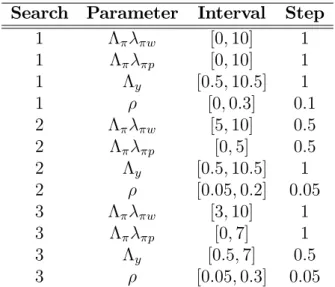
In this section, we present the results of our search for the best calibration of (5.1) and (5.2) in terms of (5.5). Given that we conduct our search in a four dimensional space, the number of potential combinations of parameter values is large at any level of discretization. We have therefore constrained our search.

Search Parameter Interval Step 1 w [0;10] 1 1 p [0;10] 1 1 y [0:5;10:5] 1 1 [0;0:3] 0:1 2 w [5;10] 0:5 2 p [0;5] 0:5 2 y [0:5;10:5] 1 2 [0:05;0:2] 0:05 3 w [3;10] 1 3 p [0;7] 1 3 y [0:5;7] 0:5 3 [0:05;0:3] 0:05

Table 5.1: Intervals for parameter value search

We looked for optimal parameter combinations on certain intervals of parameter values. We have conducted the searches reported in Table 5.1, which gives the

interval size and the size of one step within the given interval.13 _{The intervals were}

chosen after some preliminary random calibrations and also keeping in mind that the resulting rule should have a practical appeal. All other structural parameters in the model were calibrated as before. The parameter combinations we report all satisfy the Blanchard-Kahn (1980) conditions for uniqueness and stability of the results.

All of the reported three searches have selected the following calibration as

the one that provides the best …t with the optimal solution: = 10:0; p =

1:0; w = 0; y = 3:5 and = 0:20.14 The reported parameter values imply a

long-run response coe¢ cient of 1:40 at price in‡ation and a long-run coe¢ cient

13_{The precision of our grid-search is limited by the available computer power.}

14_{In this speci…c case, the coe¢ cient at lagged wage in‡ation in the targeting rule is zero.}

Results obtained through a similar exercise for di¤erent lengths of wage contract duration not reported here have, however, included a positive w: Hence the general formulation of (48).

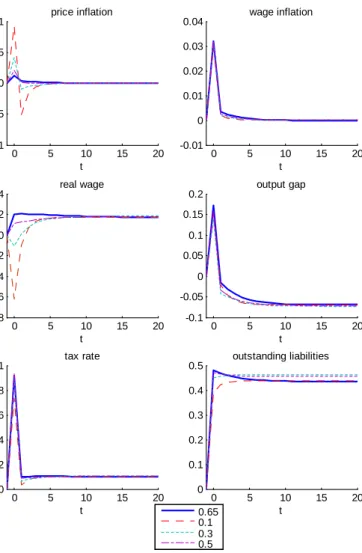
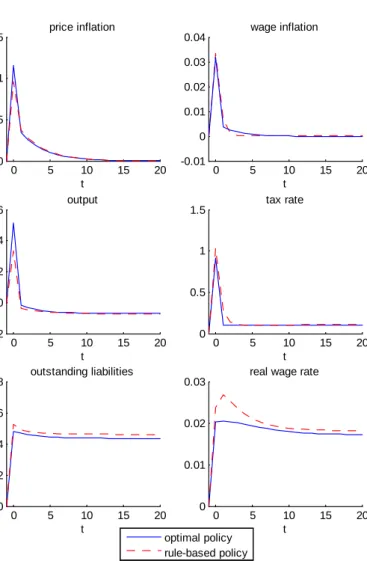
of 0:05 for wage in‡ation in the reaction function for monetary policy. The long-run response to the output gap is zero. Figure 5.1 below provides a sense of the closeness of the dynamics generated by our targeting rule-based policy and the

optimal policy.15 _{Such a close match is unlikely to be provided by a pair of simple}

instrument rules.

6. Concluding remarks

In this paper, we have extended the Benigno and Woodford (2003) economy to include staggered wage adjustment. We have shown that preferences of the policy maker can be characterized by a quadratic welfare objective involving wage in‡ation variability in addition to variability in price in‡ation and the output gap. We have shown that perfect stabilization of prices and/or wages is not a desirable way of conducting policy, if at least one of the markets is subject to nominal rigidity. We have learned that inclusion of nominal wage rigidity causes the economy’s dynamics in response to shocks to become persistent even if shocks themselves are non-persistent. The optimal dynamics of real wages is much less cyclical compared with the sticky-price, ‡exible-wage framework. The result that public debt, tax rate and the output gap are all non-stationary carries over to an economy with imperfect wage ‡exibility.

We have proposed a pair of simple speci…c targeting rules, one simple wage in‡ation rule and one real-wage-growth rule, that perform well in replicating the dynamics of the optimal economy. We have selected ‘desirable’ policies in the family of policies de…ned by these rules using a formal assessment of the match between the dynamics of the economy induced by these rules and the optimal

15_{Should one consider multiple types of shocks, the ‘desirable’ calibration of policy targets}

would likely be a¤ected and the close match with the optimal dynamics would only hold for the shocks carrying higher weight. Nevertheless, the general concept would remain una¤ected.

0 5 10 15 20 0 0.005 0.01 0.015 price inflation t 0 5 10 15 20 -0.01 0 0.01 0.02 0.03 0.04 wage inflation t 0 5 10 15 20 -0.2 0 0.2 0.4 0.6 output t 0 5 10 15 20 0 0.5 1 1.5 tax rate t 0 5 10 15 20 0 0.2 0.4 0.6 0.8 outstanding liabilities t 0 5 10 15 20 0 0.01 0.02

0.03 real wage rate

t optimal policy

rule-based policy

dynamics of the economy.

In Horvath (2007), we show that these rules perform similarly well under di¤erent calibrations of price and wage contract duration. For reasons explained in Correia et al. (2003) and Benigno and Woodford (2006a), the present framework is not likely to provide useful results for economies with more complicated tax structures, involving di¤erent types of tax instruments that could be varied independently of each other. The question of the links between the tax system and the appropriate formulation of the targeting rules remains an interesting one to explore further. In Horvath (2007), we have replicated the analysis presented in this paper for an economy in which tax is on sales revenues rather than wage income and found that optimal dynamics was best approximated by a pair of speci…c targeting rules in which the wage in‡ation rule is replaced by a price in‡ation rule. Hence, when devising appropriate targeting-rule-based frameworks, one also needs to examine carefully the link with the tax system in addition to the dynamics of the supply side of the economy.

References

[1] Aiyagari, S. R., A. Marcet, T. J. Sargent and J Seppala, 2002, Optimal Taxation without State-Contingent Debt, Journal of Political Economy, vol. 110, no. 6, 1220-1254.

[2] Amato, J. D. and T. Laubach, 2003, Rule-of-Thumb Behaviour and Monetary Policy, European Economic Review, 47, 791-831.

[3] Benigno, P. and M. Woodford, 2003, Optimal Monetary and Fiscal Policy: A Linear-Quadratic Approach, in: Gertler, M. and K. Rogo¤ (eds.), NBER Macroeconomics Annual, 271-332.

[4] Benigno, P. and M. Woodford, 2004, Optimal Stabilization Policy When Wages and Prices are Sticky: The Case of a Distorted Steaty State, NBER Working Paper No.10839

[5] Benigno, P. and M. Woodford, 2006a, Optimal In‡ation Targeting Under Alternative Fiscal Regimes, NBER Working Paper No. 12158.

[6] Benigno, P. and M. Woodford, 2006b, Linear-Quadratic Approximation of Optimal Policy Problems, NBER Working Paper No. 12672.

[7] Blanchard, O.J. and C.M. Kahn, 1980, The Solution of Linear Di¤erence Models under Rational Expectations, Econometrica, 48 (5), 1305-11.

[8] Calvo, G., 1983, Staggered Prices in a Utility-Maximising Framework, Journal of Monetary Economics, 12, 383-98

[9] Chadha, J.S., N. Janssen and C. Nolan, 2000, An Examination of UK Business Cycle Fluctuations: 1871-1997, Cambridge Working Papers in Economics No. 0024.

[10] Chadha, J.S., and C. Nolan, 2002, A Long View of the UK Business Cycle, National Institute Economic Review, 182, 72-90.

[11] Christiano, L.J., M. Eichenbaum and C.L. Evans, 1997, Sticky Price and Limited Participation Models of Money: A Comparison, European Economic Review, 41, 1201-1249.

[12] Christiano, L.J., M. Eichenbaum and C. Evans, 1999, Monetary Policy Shocks: What Have We Learned and to What End?, in: Taylor, J.B. and M. Woodford (eds.), Handbook of Macroeconomics, Vol. 1A, Elsevier

[13] Chugh, S.K., 2006, Optimal Fiscal and Monetary Policy with Sticky Wages and Sticky Prices, Review of Economic Dynamics, 9, 683-714.

[14] Correia, I.H., J.P. Nicolini and P. Teles, 2003, Optimal Fiscal and Monetary Policy: Equivalence Results, CEPR Discussion Paper No. 3730

[15] Dixit, A. and J. E. Stiglitz, 1977, Monopolistic Competition and Optimal Product Diversity, American Economic Review, 67, 297-308

[16] Erceg, C.J., D.W. Henderson and A.T. Levin, 2000, Optimal Monetary Policy with Staggered Wage and Price Contracts, Journal of Monetary Economics, 46, 281-313.

[17] Evans, G.W. and S. Honkapohja, 2006, Monetary Policy, Expectations and Commitment, Scandinavian Journal of Economics, 108 (1), 15-38.

[18] Horvath, M., 2007, Optimal Monetary and Fiscal Policy in Economies with Multiple Distortions, Ph.D. Thesis, University of St Andrews.

[19] King, R.G. and M. W. Watson, The Solution of Singular Linear Di¤erence Systems under Rational Expectations, International Economic Review, 39(4), 1015-1026.

[20] Levine, P. and D. Currie, 1987, The Design of Feedback Rules in Linear Stochastic Rational Expectations Models, Journal of Economic Dynamics and Control, 11, 1-28.

[21] Lucas, R.E., 1986, Principles of Fiscal and Monetary Policy, Journal of Monetary Economics, 17, 117-134.

[22] Lucas, R. E., Jr. and N. L. Stokey, 1983, Optimal Fiscal and Monetary Policy in an Economy without Capital, Journal of Monetary Economics, 12: 55-93. [23] Schmitt-Grohé, S. and M. Uribe, 2004a, Optimal Fiscal and Monetary Policy

under Sticky Prices, Journal of Economic Theory, 114, 198-230.

[24] Schmitt-Grohé, S. and M. Uribe, 2004b, Optimal Simple and Implementable Monetary and Fiscal Rules, NBER Working Paper No. 10253, January [25] Schmitt-Grohé, S. and M. Uribe, 2005, Optimal Fiscal and Monetary

Policy in a Medium-Scale Macroeconomic Model: Expanded Version, NBER Working Paper 11417.

[26] Siu, H.E., 2004, Optimal Fiscal and Monetary Policy with Sticky Prices, Journal of Monetary Economics, 51, 575-607.

[27] Stock, J.H. and M.W. Watson, 1999, Business Cycle Fluctuations in US Macroeconomic Time Series, in: Taylor, J.B. and M. Woodford (eds.), Handbook of Macroeconomics, Elsevier, Volume 1, Chapter 1, 3-64.

[28] Svensson, L. E. O., 2002, In‡ation Targeting: Should it be Modeled as an Instrument Rule or a Targeting Rule?, European Economic Review, 46, 771-780.

[29] Svensson, L. E. O., 2003, What Is Wrong with Taylor Rules? Using Judgment in Monetary Policy through Targeting Rules, Journal of Economic Literature, 41 (2), 426-447.

[30] Svensson, L.E.O. and M. Woodford, 2005, Implementing Optimal Policy through In‡ation-Forecast Targeting, in: Bernanke, B. and M. Woodford (eds.), The In‡ation-Targeting Debate, University of Chicago Press, 19-83.

[31] Woodford, M., 2003, Interest and Prices: Foundations of a Theory of

A. Appendix

We de…ne the values of the coe¢ cients used in the text:

k = (1 _k) (1 _k) k(1 +!k"k) for k=p; w p = p( 1) w = w !w+ 1 1 =_e 1c 1 (1 +!w) = (1 +!p) (1 +!w) w = w 1 w d = T d= Y Y;w = 1 (1 w) p w =d 1 !w+ 1 +d 1(1 + w) ( 1) d 1 w+ 1 w: qy = !+ 1 Y;w(1 +!) Y;w wd 1 1 2 1 Y;w w 2 1 1 c 1 + Y;wd 1h(1 +!)2 1 1 2+ 1 1 c 1 i; qY G = 1 1 + Y;w w d 1 1 c 1 + Y;w d 1 1 + _w c 1 1 ; q w = (1 Y;w) w "w+ Y;w d 1"w(1 +!w) w ;

q p = (1 Y;w) p "p+ Y;w d 1"p(1 +!) p : b Y_T = qY G qy b GT: b w_R;t= ( 1)qY G qy b Gt bw;t = (!+ 1₎ w 1 (!+ 1₎ qY G qy b Gt: fy = d 1 1 f =fw =d 1 ft = 1 1 qY G qy b Gt+ (1 )Et 1 X T=t T t d 1( 1)qY G qy d 1 1 qY G qy 1_+d 1 d 1 w 1 _! w+ 1 qY G qy ( 1)qY G qy b GT:

www.st-and.ac.uk/cdma

ABOUT THECDMA

TheCentre for Dynamic Macroeconomic Analysis was established by a direct grant from the University of St Andrews in 2003. The Centre funds PhD students and facilitates a programme of research centred on macroeconomic theory and policy. The Centre has research interests in areas such as: characterising the key stylised facts of the business cycle; constructing theoretical models that can match these business cycles; using theoretical models to understand the normative and positive aspects of the macroeconomic policymakers' stabilisation problem, in both open and closed economies; understanding the conduct of monetary/macroeconomic policy in the UK and other countries; analyzing the impact of globalization and policy reform on the macroeconomy; and analyzing the impact of financial factors on the long-run growth of the UK economy, from both an historical and a theoretical perspective. The Centre also has interests in developing numerical techniques for analyzing dynamic stochastic general equilibrium models. Its affiliated members are Faculty members at St Andrews and elsewhere with interests in the broad area of dynamic macroeconomics. Its international Advisory Board comprises a group of leading macroeconomists and, ex officio, the University's Principal.

Affiliated Members of the School Dr Fabio Aricò.

Dr Arnab Bhattacharjee. Dr Tatiana Damjanovic. Dr Vladislav Damjanovic. Prof George Evans. Dr Gonzalo Forgue-Puccio. Dr Laurence Lasselle. Dr Peter Macmillan. Prof Rod McCrorie. Prof Kaushik Mitra.

Prof Charles Nolan (Director). Dr Geetha Selvaretnam. Dr Ozge Senay. Dr Gary Shea. Prof Alan Sutherland. Dr Kannika Thampanishvong. Dr Christoph Thoenissen. Dr Alex Trew.

Senior Research Fellow

Prof Andrew Hughes Hallett, Professor of Economics, Vanderbilt University. Research Affiliates

Prof Keith Blackburn, Manchester University. Prof David Cobham, Heriot-Watt University. Dr Luisa Corrado, Università degli Studi di Roma. Prof Huw Dixon, Cardiff University.

Dr Anthony Garratt, Birkbeck College London. Dr Sugata Ghosh, Brunel University.

Dr Aditya Goenka, Essex University. Prof Campbell Leith, Glasgow University. Dr Richard Mash, New College, Oxford.

Prof Joe Pearlman, London Metropolitan University.

Prof Neil Rankin, Warwick University. Prof Lucio Sarno, Warwick University. Prof Eric Schaling, Rand Afrikaans University. Prof Peter N. Smith, York University. Dr Frank Smets, European Central Bank. Prof Robert Sollis, Newcastle University. Prof Peter Tinsley, Birkbeck College, London. Dr Mark Weder, University of Adelaide. Research Associates Mr Nikola Bokan. Mr Farid Boumediene. Mr Johannes Geissler. Mr Michal Horvath. Ms Elisa Newby. Mr Ansgar Rannenberg. Mr Qi Sun. Advisory Board

Prof Sumru Altug, Koç University. Prof V V Chari, Minnesota University. Prof John Driffill, Birkbeck College London. Dr Sean Holly, Director of the Department of

Applied Economics, Cambridge University. Prof Seppo Honkapohja, Cambridge University. Dr Brian Lang, Principal of St Andrews University. Prof Anton Muscatelli, Heriot-Watt University. Prof Charles Nolan, St Andrews University. Prof Peter Sinclair, Birmingham University and

Bank of England.

Prof Stephen J Turnovsky, Washington University. Dr Martin Weale, CBE, Director of the National

www.st-and.ac.uk/cdma

RECENTWORKINGPAPERS FROM THE

CENTRE FORDYNAMICMACROECONOMICANALYSIS

Number Title Author(s)

CDMA06/12 Taking Personalities out of Monetary Policy Decision Making?

Interactions, Heterogeneity and Committee Decisions in the Bank of England’s MPC

Arnab Bhattacharjee (St Andrews) and Sean Holly (Cambridge)

CDMA07/01 Is There More than One Way to be

E-Stable? Joseph Pearlman (LondonMetropolitan)

CDMA07/02 Endogenous Financial Development and Industrial Takeoff

Alex Trew (St Andrews) CDMA07/03 Optimal Monetary and Fiscal Policy

in an Economy with Non-Ricardian Agents

Michal Horvath (St Andrews)

CDMA07/04 Investment Frictions and the Relative Price of Investment Goods in an Open Economy Model

Parantap Basu (Durham) and Christoph Thoenissen (St Andrews)

CDMA07/05 Growth and Welfare Effects of

Stablizing Innovation Cycles Marta Aloi (Nottingham) andLaurence Lasselle (St Andrews) CDMA07/06 Stability and Cycles in a Cobweb

Model with Heterogeneous Expectations

Laurence Lasselle (St Andrews), Serge Svizzero (La Réunion) and Clem Tisdell (Queensland) CDMA07/07 The Suspension of Monetary

Payments as a Monetary Regime Elisa Newby (St Andrews)

CDMA07/08 Macroeconomic Implications of Gold Reserve Policy of the Bank of

England during the Eighteenth Century

Elisa Newby (St Andrews)

CDMA07/09 S,s Pricing in General Equilibrium Models with Heterogeneous Sectors

Vladislav Damjanovic (St Andrews) and Charles Nolan (St Andrews)

CDMA07/10 Optimal Sovereign Debt Write-downs Sayantan Ghosal (Warwick) and Kannika Thampanishvong (St Andrews)

CDMA07/11 Bargaining, Moral Hazard and

Sovereign Debt Crisis Syantan Ghosal (Warwick) andKannika Thampanishvong (St Andrews)

CDMA07/12 Efficiency, Depth and Growth:

www.st-and.ac.uk/cdma

CDMA07/13 Macroeconomic Conditions and Business Exit: Determinants of Failures and Acquisitions of UK Firms

Arnab Bhattacharjee (St Andrews), Chris Higson (London Business School), Sean Holly (Cambridge), Paul Kattuman (Cambridge). CDMA07/14 Regulation of Reserves and Interest

Rates in a Model of Bank Runs Geethanjali Selvaretnam (StAndrews). CDMA07/15 Interest Rate Rules and Welfare in

Open Economies

Ozge Senay (St Andrews).

CDMA07/16 Arbitrage and Simple Financial Market Efficiency during the South Sea Bubble: A Comparative Study of the Royal African and South Sea Companies Subscription Share Issues

Gary S. Shea (St Andrews).

CDMA07/17 Anticipated Fiscal Policy and

Adaptive Learning George Evans (Oregon and StAndrews), Seppo Honkapohja (Cambridge) and Kaushik Mitra (St Andrews)

CDMA07/18 The Millennium Development Goals

and Sovereign Debt Write-downs Sayantan Ghosal (Warwick),Kannika Thampanishvong (St Andrews)

CDMA07/19 Robust Learning Stability with

Operational Monetary Policy Rules George Evans (Oregon and StAndrews), Seppo Honkapohja (Cambridge)

CDMA07/20 Can macroeconomic variables explain long term stock market movements? A comparison of the US and Japan

Andreas Humpe (St Andrews) and Peter Macmillan (St Andrews) CDMA07/21 Unconditionally Optimal Monetary

Policy

Tatiana Damjanovic (St Andrews), Vladislav Damjanovic (St

Andrews) and Charles Nolan (St Andrews)

CDMA07/22 Estimating DSGE Models under

Partial Information Paul Levine (Surrey), JosephPearlman (London Metropolitan) and George Perendia (London Metropolitan)

For information or copies of working papers in this series, or to subscribe to email notification, contact: Johannes Geissler

Castlecliffe, School of Economics and Finance University of St Andrews