Energy Efficient Big Data Networks

Energy Efficient Big Data Networks

Ali Mahdi Ali Al-Salim

Submitted in accordance with the requirements for the degree of Doctor of Philosophy

The University of Leeds

School of Electronic and Electrical Engineering

The candidate confirms that the work submitted is her own, except where work which has formed part of jointly-authored publications has been included. The contribution of the candidate and the other authors to this work has been explicitly indicated below. The candidate confirms that appropriate credit has been given within the thesis where reference has been made to the work of others.

Chapter 4 is based on the work from:

Ali M. Al-Salim; Ahmed Q. Lawey; Taisir El-Gorashi, and Jaafar M. H. Elmirghani, "Energy Efficient Tapered Data Networks for Big Data Processing in IP/WDM Networks," the 17th International Conference on Transparent Optical Networks (ICTON), 2015, pp. 1-5.

Prof Elmirghani, the supervisor, suggested the study of the energy efficiency of big data processing in IP/WDM networks. The co-supervisor Dr Lawey, worked with the student on the MILP model development and revised the paper. The co-supervisor, Dr El-Gorashi, revised the paper, and worked with the student on paper preparation. The PhD student developed the model, obtained and analysed the results, and wrote paper.

And:

Ali M. Al-Salim; Ahmed Q. Lawey; Taisir El-Gorashi, and Jaafar M. H. Elmirghani, "Greening Big Data Networks: Volume Impact," the 18th International Conference on Transparent Optical Networks (ICTON), 2016, pp. 1-6.

Prof Elmirghani, the supervisor, suggested the study of big data’s volume impact on greening big data networks. The co-supervisor Dr Lawey, worked with the student on the MILP model development and revised the paper. The co-supervisor, Dr El-Gorashi, worked with the student on paper preparation. The PhD student developed the model, obtained and analysed the results, and wrote paper.

And

Al-Salim AM, Lawey AQ, El-Gorashi TE, Elmirghani JM. “Energy efficient big data networks: impact of volume and variety”. IEEE Transactions on Network and Service Management (TNSM), pp. 458-474, 2017 Dec 28.

Prof Elmirghani, the supervisor, suggested the study of big data’s volume and variety impact on greening big data networks. The co-supervisor Dr Lawey, worked with the student on the MILP model and heuristic development and revised the paper. The co-supervisor, Dr El-Gorashi, worked with the student on paper preparation. The PhD student developed the model, obtained and analysed the results, and wrote paper.

Chapter 5 is based on the work from:

Al-Salim, A., EL-Gorashi, T., Lawey, A. and Elmirghani, J.M., “Greening Big Data Networks: Velocity Impact”. IET Optoelectronics. 2017 Nov 21.

Prof Elmirghani, the supervisor, suggested the study of big data’s velocity impact on greening big data networks. The co-supervisor Dr Lawey, worked with the student on the MILP model development and revised the paper. The co-supervisor, Dr

El-Gorashi, worked with the student on paper preparation. The PhD student developed the model, obtained and analysed the results, and wrote paper.

Chapter 6 is based on the work from:

Al-Salim, A., El-Gorashi, T., Lawey, A.Q., and Elmirghani, J.M., “Greening Big Data Networks: Veracity Impact”, Springer Journal of Photonic Communications, Accepted, March 2018.

Prof Elmirghani, the supervisor, suggested the study of big data’s veracity impact on greening big data networks. The co-supervisor Dr Lawey, worked with the student on the MILP model development and revised the paper. The co-supervisor, Dr El-Gorashi, worked with the student on paper preparation. The PhD student developed the model, obtained and analysed the results, and wrote paper.

This copy has been supplied on the understanding that it is copyright material and that no quotation from the thesis may be published without proper acknowledgement.

I Acknowledgements

I would like to sincerely thank my supervisor, Professor Jaafar Elmirghani for his inestimable assistance and patience throughout my PhD journey. His insights and valuable advice paved the road toward accomplishing the goals of this work.

I am truly grateful to my co-supervisor, Dr. Ahmed Lawey, for the patient guidance, encouragement and immeasurable advice he has provided throughout my time as his student. I would like to acknowledge Dr. T. H. El-Gorashi, my co-supervisor for her advice and useful discussions.

I would like to acknowledge the Higher Committee for Education Development in Iraq (HCED) for funding my Ph.D.

I am indebted to my two angels, my daughter Zainab, my son Mahdi; and my beloved wife Howraa for their everlasting support and love through all stages of my life and especially during my Ph.D.

I wish to express my love and gratitude to all my family, specially my beloved mother, Rajiha, and my wonderful father, Mahdi, my soul mate sister, Anfal, my kind brothers Salwan, Radhwan and Karrar, my father in law, Mahdi, my mother in law, Najat, for their support, patience and understanding during my Ph.D.

Finally, I thank all my friends with special thanks to all my colleagues for their friendship, input and valuable discussions.

II Abstract

The continuous increase of big data applications in number and types creates new challenges that should be tackled by the green ICT community. Data scientists classify big data into four main categories (4Vs): Volume (with direct implications on power needs), Velocity (with impact on delay requirements), Variety (with varying CPU requirements and reduction ratios after processing) and Veracity (with cleansing and backup constraints). Each V poses many challenges that confront the energy efficiency of the underlying networks carrying big data traffic. In this work, we investigated the impact of the big data 4Vs on energy efficient bypass IP over WDM networks. The investigation is carried out by developing Mixed Integer Linear Programming (MILP) models that encapsulate the distinctive features of each V. In our analyses, the big data network is greened by progressively processing big data raw traffic at strategic locations, dubbed as processing nodes (PNs), built in the network along the path from big data sources to the data centres. At each PN, raw data is processed and lower rate useful information is extracted progressively, eventually reducing the network power consumption. For each V, we conducted an in-depth analysis and evaluated the network power saving that can be achieved by the energy efficient big data network compared to the classical approach. Along the volume dimension of big data, the work dealt with optimally handling and processing an enormous amount of big data Chunks and extracting the corresponding knowledge carried by those Chunks, transmitting knowledge instead of data, thus reducing the data volume and saving power. Variety means that there are different types of big data such as CPU intensive, memory intensive, Input/output (IO) intensive, CPU-Memory intensive, CPU/IO intensive, and

III

memory-IO intensive applications. Each type requires a different amount of processing, memory, storage, and networking resources. The processing of different varieties of big data was optimised with the goal of minimising power consumption. In the velocity dimension, we classified the processing velocity of big data into two modes: expedited-data processing mode and relaxed-data processing mode. Expedited-data demanded higher amount of computational resources to reduce the execution time compared to the relaxed-data. The big data processing and transmission were optimised given the velocity dimension to reduce power consumption. Veracity specifies trustworthiness, data protection, data backup, and data cleansing constraints. We considered the implementation of data cleansing and backup operations prior to big data processing so that big data is cleansed and readied for entering big data analytics stage. The analysis was carried out through dedicated scenarios considering the influence of each V’s characteristic parameters. For the set of network parameters we considered, our results for network energy efficiency under the impact of volume, variety, velocity and veracity scenarios revealed that up to 52%, 47%, 60%, 58%, network power savings can be achieved by the energy efficient big data networks approach compared to the classical approach, respectively.

IV

Table of Contents

Acknowledgements ... I Abstract ... II

Table of Contents ... IV List of Figures ... VII List of Tables ... IX List of Abbreviations ... X Chapter 1 Introduction... 1 1.1 Research Objectives ... 6 1.2 Original Contributions ... 6 1.3 Related Publications... 9 1.4 Thesis Structure ... 10

Chapter 2 Optical Networks ... 12

2.1 The Evolution of Optical Networks ... 12

2.2 WDM Switching Technology ... 16

2.2.1Optical circuit switching (OCS)... 16

2.2.2Optical packet switching (OPS) ... 16

2.2.3Optical burst switching (OBS) ... 17

2.2.4Optical label switching (OLS) [16]... 18

2.3 IP over WDM ... 18

2.4 Energy-Efficiency in Optical Networks ... 20

2.4.1Introduction ... 20

2.4.2Power consumption problem and energy efficiency solutions ... 21

2.5 Energy Minimisation in Core Networks ... 22

2.5.1Selectively turning off network elements ... 24

2.5.2Energy-efficient network design ... 25

2.5.3Green routing ... 26

2.6 Linear Programming ... 27

2.7 Linear Programming Capabilities ... 27

2.8 A Linear Program General Form ... 28

2.9 Simplex Optimisation ... 29

2.10 Adapting Model to the Simplex Method [63] ... 30

V

2.11.1 Link-path formulation ... 31

2.11.2 Node-link formulation ... 34

2.12 Summary ... 37

Chapter 3 Energy Efficient Big Data Networks ... 38

3.1 Understanding Big Data ... 38

3.1.1Big data sources [67] ... 38

3.1.2The main of characteristics big data ... 39

3.2 Hadoop-MapReduce: The Storage and Processing Platform for Big Data44 3.2.1Hadoop-MapReduce ... 44

3.2.2Implementing Hadoop-MapReduce [79] ... 45

3.3 Network Architecture Utilised by Big Data... 47

3.3.1Challenges of big data processing ... 49

3.4 Related Work: Networks and Big Data Processing Solutions ... 50

3.4.1Big data in social networks ... 51

3.4.2Big data in I/O environments ... 52

3.4.3Big data storage and segmentation ... 52

3.4.4Local gathering and processing of big data in access networks (user-level) ... 53

3.4.5Big data in aggregation networks (bridge-level) ... 54

3.4.6Processing and transporting big data in geo-distributed networks (datacentres level) ... 54

3.4.7Energy efficient cloud computing services in optical networks and big data transfer in elastic optical networks (EON) ... 58

3.5 The Proposed Energy Efficient Big Data Networks (EEBDN) ... 59

3.5.1EEBDN: An illustrative example... 63

3.6 Summary ... 66

Chapter 4 Energy Efficient Big Data Networks: The Impact of Volume and Variety ... 67

4.1 Energy Efficient Big Data Networks: Impact of Volume ... 67

4.1.1Problem statement ... 69

4.1.2Volume MILP model ... 69

4.1.3Volume heuristic ... 84

4.1.4Complexity analysis ... 87

4.2 Results of Volume Scenarios ... 88

4.2.1Scenario #1: Deterministic Chunks volume, PRR = 0.001, number of servers per PN = 5-15 servers ... 89

VI 4.2.2Scenario #2: Deterministic Chunks volume, PRR = 0.001, number of

servers per PN = 10-30 servers ... 95

4.3 Assessing the Energy Efficiency Limits of PNs in the EEBDN ... 98

4.3.1Results ... 99

4.4 Software Matching Problem and Its Effect on EEBDN Performance .. 101

4.4.1MILP model extension description ... 102

4.4.2Results ... 102

4.5 Energy Efficient Big Data Networks: Impact of Variety... 105

4.5.1Variety MILP model ... 105

4.5.2Results of variety scenarios ... 105

4.6 Assessing the EEBN by Considering Different Power Profiles ... 113

4.7 Summary ... 115

Chapter 5 Energy Efficient Big Data Networks: Impact of Velocity ... 117

5.1 Velocity MILP Model ... 120

5.2 Velocity Model Results... 124

5.2.1Scenario #1: Deterministic volume and RCET per Chunk ... 124

5.2.2Scenario #2: Different volume, PRR and RCET per Chunk ... 130

5.3 Summary ... 133

Chapter 6 Energy Efficient Big Data Networks: Impact of Veracity ... 135

6.1 Veracity MILP Model Description ... 136

6.2 Veracity Model Results... 142

6.2.1Scenario #1: Veracity with large enough storage capacity ... 142

6.2.2Scenario #2: Veracity with limited storage capacity per PN ... 145

6.3 Summary ... 148

Chapter 7 Conclusions and Future work... 149

7.1 Conclusions ... 149

VII

List of Figures

Figure 2-1: Time division multiplexing (TDM). ... 13

Figure 2-2: Frequency division multiplexing (FDM). ... 14

Figure 2-3: Wavelength division multiplexing (WDM). ... 15

Figure 2-4: Optical burst switching network. ... 17

Figure 2-5: IP over WDM network. ... 19

Figure 2-6: (a) A three node network example (b) All possible paths for the three-node example. ... 32

Figure 2-7: Demand flow view between nodes 1 and 2. ... 34

Figure 3-1. Big data sources [67]. ... 40

Figure 3-2: The four Vs of big data [69]. ... 41

Figure 3-3: Volume of data is increasing, while the percentage of data that can be processed is declining [65]. ... 42

Figure 3-4: Hadoop MapReduce architecture. ... 46

Figure 3-5: The network architecture utilised by big data. ... 48

Figure 3-6. (a) The CBDN. (b) The EEBDN [104]. ... 60

Figure 3-7: EEBDN: An illustrative example. ... 64

Figure 4-1. NSFNET network with PNs ... 70

Figure 4-2: EEBDN: volume heuristic. ... 86

Figure 4-3 (a) CBDN power consumption vs EEBDN power consumption (MILP and heuristic) for volume Scenario #1. (b) Utilisation of processing capacity % in the EEBDN with different values of β for volume Scenario #1. ... 92

Figure 4-4: The COST239 network, and (b) the Italian network. ... 94

Figure 4-5: CBDN power consumption vs EEBDN power consumption (a) COST239 network, (b) Italian network. ... 94

Figure 4-6: (a) CBDN power consumption vs EEBDN power consumption for volume Scenario 2. (b) Utilisation of processing capacity % in EEBDN with different values of β for volume Scenario 2. ... 97

Figure 4-7: CBDN power consumption vs EEBDN power consumption when PNs equipment consume more power than DCs equipment at PRR=0.001 and PRR=0.6 with β=30. ... 100

Figure 4-8: Software packages availability and its impact on EEBDN performance at β=10. ... 103

VIII Figure 4-9: (a) The CBDN power consumption vs the EEBDN power consumption for

variety Scenario #1. (b) Utilisation of processing capacity % in EEBDN with different values of β for variety Scenario #1. ... 107 Figure 4-10: Sample of input data for variety Scenario #2 for node #8 at β = 10. . 109 Figure 4-11: (a) CBDN power consumption vs EEBDN power consumption for variety

Scenario #2. (b) Utilisation of processing capacity % in the EEBDN with different values of β for variety Scenario #2. ... 111 Figure 4-12: CBDN power consumption vs EEBDN power consumption of 2010, 2020

BAU, and 2020 BAU+GT power profiles. ... 114 Figure 5-1: (a) Network power consumption for the CBDN and EEBDN vs ф when

CHs=100, for velocity Scenario #1. (b) Max and Min CPU execution time needed to process the Chunks in the network vs Ф when CHs=100, for velocity Scenario #1. ... 129 Figure 5-2: (a) Network power consumption for the CBDN and EEBDN vs ф when

CHs=100, for velocity Scenario #2. (b) CPU execution time (Tp) allocated to process Chunks at each PN and each DC vs ф when CHs=100, for Scenario #2. ... 132 Figure 6-1 Architectural framework for big data analytics [133]. ... 136 Figure 6-2 (a). Network power consumption for the CBDN and EEBDN with and

without BN for veracity Scenario #1. (b). Storage used in the PNs and DCs and BN with different values of β for veracity Scenario #1. ... 144 Figure 6-3 (a) PNs storage size with different values of β for veracity Scenario #2. (b)

Utilisation of processing capacity for different values of β when considering limited storage per PN for veracity Scenario #2. (c)Network power consumption for the CBDN and EEBDN with and without BN with limited storage per PN for veracity Scenario #2... 147

IX

List of Tables

Table 3-1. MapReduce Facebook Cluster Summary [23]. ... 63

Table 4-1: List of parameters and their definitions. ... 74

Table 4-2: List of variables and their definitions. ... 75

Table 4-3: Input data for volume MILP model. ... 89

Table 4-4: Volume Scenario #1 parameters. ... 90

Table 4-5: Volume Scenario #2 parameters. ... 95

Table 4-6: List of parameters and their definitions. ... 102

Table 4-7: Variety Scenario #1 parameters. ... 106

Table 4-8: Variety Scenario #2 parameters. ... 108

Table 4-9. Variety Scenarios Summary. ... 113

Table 4-10 Power Consumption Values. ... 114

Table 5-1: List of parameters and their definitions. ... 121

Table 5-2: List of variables and their definitions. ... 121

Table 5-3: Velocity Scenario #1 parameters. ... 125

Table 5-4: Velocity Scenario #2 parameters. ... 131

Table 6-1: List of variables and their definitions. ... 137

X

List of Abbreviations

ACET Allocated CPU Execution Time

ACET Allocated CPU execution time of a Chunk AWP Allocated Processing Workload

CBDN Classical Big Data Networks CCC Couple Congestion Control CDM Code Division Multiplexing CDN Content Distribution Networks CET CPU Execution Time

CHT Chunk Big Data Traffic CMS Compact Muon Solenoid CPI Cycles per Instruction DC Data Centre

EEBDN Energy Efficient Big Data Networks EON Elastic Optical Networks

EXC Electronic Cross-connect; Electronic Core Packet Switch GHG Green House Gases

IC Instruction Count

ICT Information and Communication Technologies INF Info Big Data Traffic

IO Input/Output IP Internet Protocol

IPN Intermediate Processing Node ISP Internet Service Provider

XI LHC Large Hadron Collider

MILP Mixed Integer Linear Programming MPTCP Multipath Transmission Control Protocol MR Malleable Reservation

NFV Network Function Virtualization NPC Network Power Consumption OCS Optical Circuit Switching OLS Optical Label Switching OPS Optical Packet Switching OSPF Open Shortest Path First OXC Optical Cross Connect PBS Optical Burst Switching

PN Processing Node

PPR Processing Reduction Ratio PUE Power Usage Effectiveness PW Processing Workload

RCET Requested CPU Execution Time

RCET Requested CPU execution time of a Chunk RSA Routing and Spectrum Assignment

RWP Requested processing workload for a Chunk SDH Synchronous Digital Hierarchy

SONET Synchronous Optical Networks SPN Source Processing Node TDM Time Division Multiplexing

XII WDM Wavelength Division Multiplexing

1

Chapter 1 Introduction

In recent years, energy crises and environmental protection are under the spotlight, specifically, the remarkable growth of energy consumption in ICT (Information and Communication Technologies). According to [1], in the first quarter of 2007, British Telecom consumed about 0.7% of the total UK’s power consumption and therefore was the largest single power consumer in the UK. In the same line, about 8% of the total electricity in the United States is being consumed by information and communication technologies [2], and an increase of more than 4% per year has been predicted.

So far, applications such as telework telecom applications, video conferencing, e-commerce, and their impact on human movements, have stamped ICT as an environment-friendly sector, however, there is a downside of ICT. Due to the ICT availability, everywhere and anywhere in our daily life, (both private and professional), the power that is needed to maintain and operate the network is being considered as an essential problem associated with bandwidth growth. Another aspect, energy consumption of computers and network equipment is becoming a significant part of the global energy consumption as a result of the network expansion [3]. For example, during the last decade, the Internet bandwidth has increased by approximately 50 to 100 times [4], and accordingly, the network power consumption has increased simultaneously. Thus, lots of attention is being focused on “energy-aware” ICT solutions [3]. One of the most significant current discussions in today’s ICT sector is the increase in energy consumption due to the massive increase in the number of devices accessing the Internet – with around 40% of the world population having an Internet connection [5] – and the huge amount of generated data. Data centre power

2 consumption is in the range of 100-130 GWh per year, as measured by the power usage effectiveness (PUE) index, and computer room air conditioning consumes up to half the total power consumed by the data centre [6]. The amount of data created between the period of the dawn civilisation and 2003 is estimated to be five Exabyte. Currently, the same amount of data is created every two days [7]. This massive increase in generating data and the huge data generated is referred to as big data.

Data scientists classify big data into four main categories (4Vs): volume (implies enormous volumes of data), variety (refers to the many sources and types of data) velocity (deals with the pace at which data flows from source), and veracity (refers to the biases, noise and abnormality in data). Each V carries many challenges that have implications on the power consumption of the underlying networks carrying the big data traffic.

The first challenge facing the Data Centres (DCs) is the enormous Volume of data fluxing to them. Voluminous growth in generating big data is causing drops in the percentage of processed data of organisations due to the lack of resources and poor analysis tools [8]. Thus, a large amount of the data that is to be processed is either neglected, deleted or delayed. Hence, there is unnecessary networking power consumption, extra wastage of storage and bandwidth because of transferring raw data, which leads to increasing the financial and environmental costs.

Variety means that there are different types of big data applications such as CPU intensive, memory intensive, Input/output (IO) intensive, CPU-Memory intensive, CPU/IO intensive, and memory-IO intensive applications. Each application requires different amounts of processing,

3 memory, storage, and networking resources. These different types come from the diversity of big data sources, such as healthcare sensors, smart devices, social networks [8].

Velocity is data in motion, which is the speed at which data is fluxing in and processed in the DCs. High-speed processing of such immense data volumes as produced by plentiful data sources calls for new processing and communications methodologies in the big data era. The processing velocity of big data can be classified into two modes: expedited-data processing mode and relaxed-data processing mode. Expedited-data processing mode is used for the CPU hungry applications that need to be processed in real time [9], e.g. remote patient monitoring. Relaxed-data processing mode can tolerate some delay and can be processed in a batch processing mode after being stored inside DCs, such as digital image processing and automated transaction processing.

Veracity of big data is a more serious challenge to data scientists since they need to distinguish between the meaningful data and the dirty data [10]. Low-quality data causes the U.S. economy to waste $3.1 trillion each year [10]. Veracity specifies trustworthiness, data protection, data backup, and data cleansing constraints. Data cleansing [11] deals with detecting and removing dirty data due to overlaps, errors, duplications, and contradictory materials from big data to improve its quality. It provides easy access to accurate, consistent and consolidated data of different data forms.

Significant efforts have been dedicated to optimise the power consumption of conventional data centres and the power consumption and communication cost of big data networks including energy-efficient data centre designs [12, 13], energy-efficient inter- and intra-data centre network

4 architectures [14, 15], designing energy-efficient cloud computing services and energy-efficient resource provisioning, and virtual network embedding for cloud systems [16, 17], minimisation of overall cost for Big Data placement, processing, and movement across geo-distributed data centres

[18-20], and minimisation of the communication cost of big data queries and real-time big data

processing on the heterogeneous systems [21, 22].

To understand the usefulness of our proposed Energy Efficient Big Data Networks (EEBDN) concept, consider an example of a Classical Big Data Network (CBDN), where all the big data Chunks Traffic (CHT); which is the unprocessed big data traffic, generated by the source nodes is forwarded to the DCs to be processed there. On the other hand, in the EEBDN, a progressive processing technique is implemented to process the CHT at strategic locations, dubbed Processing Nodes (PNs), built into the network along the path from the data source to the destination. Our progressive processing can be classified into three main stages: edge processing stage, which is implemented in the Source PNs (SPNs), intermediate processing stage, implemented in the Intermediate PNs (IPNs), and central processing stage, implemented in the DCs. During the processing of big data, the extracted information from the CHT raw traffic, referred to as Info traffic (INF), is smaller in volume compared to the original big data traffic each time the data is processed, hence, reducing network power consumption.

Typically, the size of Info is very small compared to the size of Chunks [23] in many big data applications such as remote patient monitoring, where info is used for example to capture only the abnormality in the heartbeat from a huge amount of measured heartbeat rate time series. Processing Nodes (PNs) are attached to the core nodes. Each PN is composed of internal switches

5 and routers, limited storage, and a limited number of servers depending on the available building space and its structure is similar to the cloud structure in [16]. DCs, however, are assumed to have large enough processing and storage capabilities. PNs are capable of processing different amount of big data traffic depending on their processing and storage capacity.

For energy efficiency in big data networks, the work in this thesis presents detailed analyses of the process of big data applications inside the PNs by considering the 4 Vs of big data and exemplifies its implication in the EEBDN. The approach exploits energy-efficient processing of big data Chunks along the path from the source to the destination, starting from the SPNs, moving through the IPNs, and finally reaching the DCs. This approach showed the impact of increasing the total resources utilisation (such as PNs’ and DCs’ servers, switches, and routers), which reduced the overall energy consumption. Furthermore, this approach showed the impact of processing the CHT, (which typically contained large data volume, along the way from source data nodes to the destination) on the network power consumption.

The extracted knowledge from the CHT (i.e. the INF) is typically smaller in size, and this led to a significant reduction in big data traffic each time the data is processed, hence, reducing the network power consumption. The benefits were maximised using a mixed integer linear programming (MILP) mathematical optimisation, and a heuristic was developed and used to verify the MILP optimisation. The goal of the optimisation was to ensure that power consumption is minimised by effectively considering the distinct features of each V as mentioned earlier.

6

1.1 Research Objectives

The following primary objectives were set for the work reported in this thesis: 1. To design a network architecture that supports energy-efficient big data processing

by building Processing Nodes (PNs).

2. To develop a scheme for the transmission and processing of enormous volumes of big data, starting at processing nodes close to the data source, with significant processing resources provided at centralised data centres.

3. To capture the distinct features of big data’s variety by evaluating the energy efficiency implications of processing various big data applications in networks where edge, intermediate, and finally central processing in networks is considered. 4. To utilise the proposed network architecture to handle the challenges of the

velocity dimension of big data where data can have expedited or relaxed processing requirements.

5. To investigate the impact of the veracity dimension on energy efficient big data networks by performing the cleansing operation in the proposed network architecture before processing big data applications such that the data is readied for big data processing.

1.2 Original Contributions

The main contributions of this thesis are as follows:

1. We introduced MILP models to minimise the power consumption of networks that include processing nodes considering the impact of volume and variety of big data in IP over WDM core networks. As a result, we made the following contributions:

7 (i) we evaluated, using MILP and heuristic, the volume dimension by analysing

the optimal distribution of big data volumes in different processing locations that have different processing capabilities where Chunks demand similar processing and yield similar volume reduction ratios; (ii) we examined, using MILP, the impact of variety by considering the case where different CPU workloads are required to serve different volumes of Chunks at different volume reduction ratios; (iii) we used our progressive processing technique to optimise the processing locations of the big data Chunks and compared the results to the classical technique where no PNs exist in the network. The processing locations are optimally chosen at either SPNs, inside “location optimised” DCs or at the IPNs. Thus, we jointly minimised the power consumption of the overall network and processing resources since the network elements, e.g., router ports, the routing paths, and the processing resources, have their energy efficiently utilised; (iv) we assessed the impact of the energy efficiency of PNs hardware on the proposed energy efficient big data networking approach where the PNs constituents (LAN switches, routers, and servers) consume higher power compared to data centre equipment; (v) we considered a software matching problem to evaluate the performance limits of our approach where each PN contains different software packages used to process different big data applications.

2. We developed a MILP model to jointly minimise the power consumption of the network and the power consumption of the processing of information given the velocity dimension of big data. We considered bypass IP over WDM core

8 networks with our progressive processing approach. As a result, we made the

following contributions: (i) we explored the impact of the big data processing velocity dimension on the IP over WDM network energy efficiency considering an expedited-data processing mode and a relaxed-data processing mode, (ii) we used our progressive processing technique to process big data Chunks and compared the results to the classical approach where progressive processing is not allowed. In our approach, the processing locations are optimally selected at the SPNs, at the IPNs or inside the centralised data centres (DCs). As a result, a significant reduction in the network power consumption is achieved each time the data is processed along the journey from the source to the DCs.

3. We developed a MILP model to jointly minimise the power consumption of the network and the power consumption of the processing of information given the veracity dimension of big data. Here we considered the power consumption of bypass IP over WDM core networks and the power consumption of processing nodes. As a result, we made the following contributions: (i) we studied the influence of Veracity by performing cleansing and backup for big data Chunks before processing, where a Backup Node (BN) location is optimally selected to store a copy of the cleansed big data Chunks; (ii) we employed our energy efficient edge, intermediate, and centralised processing technique to process the cleansed Chunks in optimal locations in the core network and compared the results to the classical approach that lacks progressive processing. The optimally selected processing locations for the energy efficient approach are either the SPNs where

9 Chunks are generated, inside location optimised DCs, or at the IPNs, between the

SPNs and the DCs. Accordingly, the network elements, e.g., router ports, the routing paths, and the processing resources, are efficiently utilised to jointly minimise the power consumption of the overall network and processing resources.

1.3 Related Publications

The original contributions in this thesis are supported by the following publications:

 Journals

1. Al-Salim, A., EL-Gorashi, T., Lawey, A. and Elmirghani, J.M., “Greening Big Data Networks: Velocity Impact”. IET Optoelectronics. 2017 Nov 21.

2. Al-Salim AM, Lawey AQ, El-Gorashi TE, Elmirghani JM. “Energy efficient big data networks: impact of volume and variety”. IEEE Transactions on Network and Service Management (TNSM), pp. 458-474, 2017 Dec 28.

3. Al-Salim, A., El-Gorashi, T., Lawey, A.Q., and Elmirghani, J.M., “Greening Big Data Networks: Veracity Impact”, Springer Journal of Photonic Communications, Accepted, March 2018.

 Conferences

4. A. M. Al-Salim, A. Q. Lawey, T. El-Gorashi, and J. M. Elmirghani, "Energy Efficient Tapered Data Networks for Big Data Processing in IP/WDM Networks," in Transparent Optical Networks (ICTON), 2015 17th International Conference on, 2015, pp. 1-5.

10 5. A. M. Al-Salim, H. M. Mohammad Ali, A. Q. Lawey, T. El-Gorashi, and J. M. Elmirghani, "Greening Big Data Networks: Volume Impact," in Transparent Optical Networks (ICTON), 2016 17th International Conference on, 2016, pp. 1-6.

1.4 Thesis Structure

Following the introduction in Chapter 1, the rest of the thesis is organised as follows:

Chapter 2 reviews optical networks, energy efficient optical networks, mixed integer linear programming (MILP), IP over WDM networks, and provides an overview of the main topics related to the work on energy efficiency in optical networks.

Chapter 3 discusses the main sources of big data, big data characteristics, Hadoop-MapReduce scheme, and reviews the work on big data processing and networking. Attention is given to the related work on minimising communication cost and energy efficiency in big data networks. A special section is dedicated to introducing the proposed topics on energy efficient big data networks and comparison with the classical networks with an illustrated example.

Chapter 4 introduces a MILP model and a heuristic to examine the impact of big data’s volume on energy efficient big data networks. It also introduces a MILP model to examine the impact of the big data’s variety dimension on energy efficient big data networks.

Chapter 5 introduces a MILP model that focuses on power minimisation in big data networks given the big data’s velocity requirements.

Chapter 7 introduces a MILP model to minimise big data networks and processing power consumption given the veracity dimension of big data.

11 The thesis concludes in Chapter 7, which summarises this work’s main contributions and gives recommendations for future work.

12

Chapter 2 Optical Networks

The globalisation of the Internet and the boom in high bandwidth applications such as video streaming and Big Data applications has greatly accelerated the call to develop the communications infrastructure. Accordingly, such huge bandwidth requirements have gradually resulted in developing the bandwidth supported by the optical fibre to reach its current maximum of 1.050 petabit/s over 52.4 km of 12-core (light paths) optical fibre [24]. Nowadays, the optical fibre is the dominant medium which can handle such immensely growing traffic. This is because of its many advantages compared to copper and wireless mediums such as high reliability and low signal attenuation.

2.1 The Evolution of Optical Networks

In 1965 fibre optics has come to the light and this has been considered as the start of networks revolution [25]. Since then to present, the development in optical networks has undergone two main phases: Phase one is related to the transmission where the optical fibre is used only to transmit huge traffic in peer to peer fashion while the routing and switching are electronic devices responsibility. That was the era of Synchronous Optical Networks (SONET) and Synchronous Digital Hierarchy (SDH) [26].

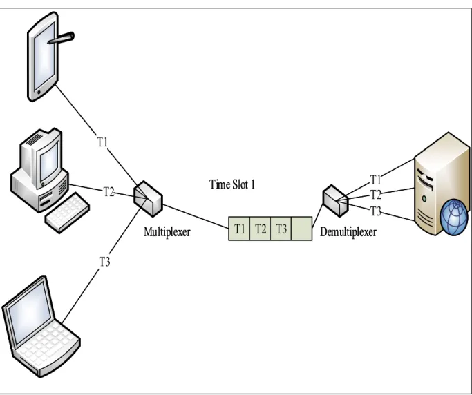
Phase two has witnessed the revolution with the introduction of multiplexing techniques such as Time Division Multiplexing (TDM), Frequency Division Multiplexing (FDM), Code Division Multiplexing (CDM), and Wavelength Division Multiplexing (WDM) [26]. TDM specifies time slots for users to transmit data over a single communication channel with fixed bit rate as shown

13 in Figure 2-1 [27]. This technique helps to utilise all the available bandwidth but users’ data may be delayed depending on the time slot window.

Multiplexer

Demultiplexer

T1

T2

T3

T2

T1

T3

Time Slot 1

Multiplexer

Demultiplexer

T1

T2

T3

T2

T1

T3

Time Slot 1

T2 T3

T1 T2 T3

T1

Figure 2-1: Time division multiplexing (TDM).

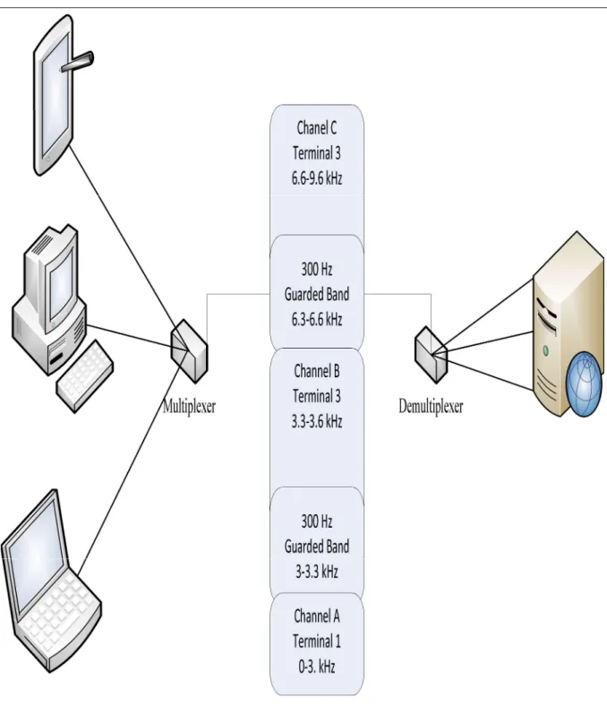
FDM [28] divides the total bandwidth of the system into different sub-channels without overlapping and this technique is useful when transmitting different requests at the same time but at a lower bit rate per request as shown in Figure 2-2.

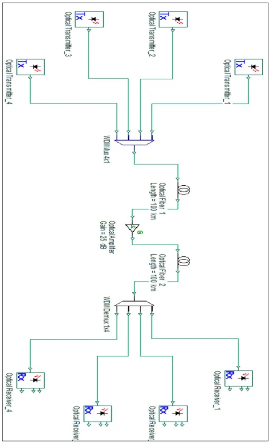
WDM [26, 29, 30] is a technique that enables multiple data stream to be sent on multiple wavelengths as shown in Figure 2-3. In WDM, the spectrum of the transmitted signals is divided

14 a specific communication channel operating at maximum electronic speed, and this allows the huge bandwidth of optical fibre to be utilised [30].

15 Figure 2-3: Wavelength division multiplexing (WDM).

16

2.2 WDM Switching Technology

Basically, there are four types of switching technology in WDM networks which are Optical Circuit Switching (OCS), Optical Packet Switching (OPS), Optical Burst Switching (OBS), and Optical Label Switching (OLS).

2.2.1 Optical circuit switching (OCS)

OCS can be defined as a source-destination permanent connection. Each connection requires dedicated path or a guaranteed amount of bandwidth and a wavelength all time [31, 32].

The sum of the bandwidth of all connections should be less or equal to the total link bandwidth. Before a source starts sending data to a destination, a Routing and Wavelength Assignment [26] algorithm, [31] assigns specific wavelengths and route to the lightpath.

The pros of OCS lie in assigning dedicated wavelengths during the transmission process, which is useful in terms of reliability and security for real-time applications. While the cons of this technique lie in utilising a portion of the total bandwidth which means that the remaining bandwidth is useless until the circuit is released. Moreover, there is delay in establishing the connection before the transmission process, which might be inappropriate for delay-sensitive applications.

2.2.2 Optical packet switching (OPS)

OPS is a technique in which different data segments from different users can share the same wavelength and there is no wavelength reservation and no wasted connection capacity. OPS can be divided into two types: synchronous and asynchronous. The size of packets in the synchronous

17 approach are fixed and each packet should contain synchronisation bits. While in the asynchronous technique the size of packets is flexible with no synchronisation clock required between sender and receiver [26, 33, 34]. The first approach is used for delay sensitive applications while the second one is not.

2.2.3 Optical burst switching (OBS)

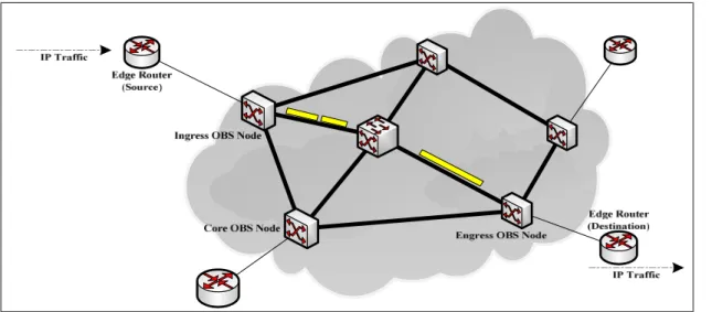
Traffic in the optical network is greatly increasing and this requires very fast switching in the order of few nanoseconds [33, 35, 36]. OBS combines the merits of both OCS and OPS and may be efficient as it first does not need packet switching buffering but it may also not utilise the whole wavelength band resulting in wastage. OBS includes two packets, control packet, and data burst packet. The control packet is used to establish the path for the data burst. This is done by sending this packet along the route to the destination node. It is processed electronically at the core network nodes to decide a specific route for each data burst packet. The ingress OBS node then gathers these data burst packets, which have different size and sends them to the destination as shown in Figure 2-4.

18

2.2.4 Optical label switching (OLS) [16]

OLS combines the benefits of optical burst switching OBS and optical packet switching OPS and overcomes their disadvantages [37-39]. It can hold-up both packets and bursts by assigning different labels for each of them. Before sending data, OLS ensures a lightpath between source and destination is established. This is done by sending a signal to the control layer to establish a Label Switching Path (LSP). Generally, all packets carrying the same label should be transmitted through the same LSP. When a packet passes through intermediate switching nodes and reaches the edge router, it is assigned a new label by this router according to the labels stored in the router using the forwarding labels table. The packets with new labels are forwarded to their destinations according to the label forwarding table.

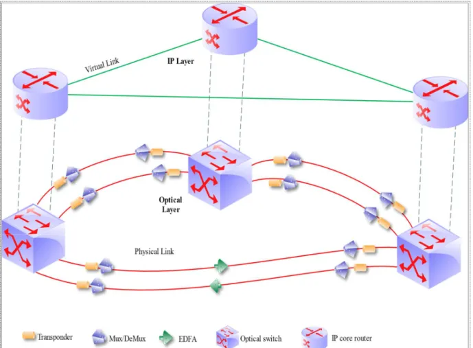
2.3 IP over WDM

The IP over WDM network is comprised of two layers the IP layer and the optical layer as shown in Figure 2-5. The IP layer consists of a core IP router connected to an optical switch. The IP router aggregates data traffic from low-end access routers. The optical layer provides the needed huge capacity and bandwidth for the communications between IP routers [40]. Optical switches are connected to physical fibre links, and each link may contain multiple fibre strands. Each fibre is supplemented by: pair of wavelength multiplexer/demultiplexers required to multiplex/demultiplex wavelengths; transponders that can provide optical/electrical/optical (OEO) conversion and hence also full wavelength conversion at each core node; and, for long distance transmission, Erbium Doped Fiber Amplifiers (EDFAs) are used to amplify the optical signal. An automatically controllable optical cross-connect (OXC) switch is used as the core optical switch box or a dumb optical patch panel can be used instead [25, 41].

19 Figure 2-5: IP over WDM network.

IP over WDM networks can be realised in two ways: Lightpath non-bypass and lightpath bypass. Considering lightpath non-bypass, the lightpath must be dropped at each intermediate node and all the data carried by a lightpath must be processed and forwarded by all IP routers on its path to the destination node. In contrast, the lightpath bypass approach uses a cut-through lightpath, where a lightpath directly bypasses intermediate nodes. Only destination node IP router processes the lightpath data. This requires the optical nodes to have intelligence to bypass lightpaths destined to other nodes. The implementation of lightpath bypass however has the advantage of introducing a significant reduction in the number of working IP router ports [42, 43]. The communications between core routers are directly over lightpaths, where each lightpath joins a pair of router ports,

20 and lightpaths are considered virtual links for the IP layer. IP routers play a major role in the total energy consumption in an IP over WDM transport network. Thus, minimising the required number of IP router ports can potentially maximise the energy consumption saving in an IP over WDM network [42, 43].

2.4 Energy-Efficiency in Optical Networks

2.4.1 Introduction

Today, most of the energy need is being provided by traditional energy sources, such as hydrocarbon energy sources. According to [3], about 85 percent of the primary energy of USA’s electricity is provided using this source, however, this energy is not renewable, and its use is expected to be finally minimised. Also, large amounts of Green House Gases (GHG), the main reason for Global Warming, are emitted because of the combustion of hydrocarbon materials. Thus, hydrocarbon energy sources utilisation should be minimised. If traditional energy sources such as coal or natural gas are used, a network component that consumes 1 kWh of such traditional electrical energy emits approximately 228 grams of CO2 to nature [4]. The latest report of

SMARTer2030 estimates that the ICT emissions could be reaching 1.25Gt CO2e in 2030 or 1.97% of global emissions [44]

In order to address this important problem, mutual responsibility requires both network operators and system vendors, alike, to corporate in order to reduce the carbon footprint and reduce the environmental impact of communication networks [45]. In [4], the use of renewable energy has been proposed to reduce the CO2 emissions at a given energy consumption level. A Linear

21 renewable energy is used and a novel heuristic was proposed for improving renewable energy utilisation. While the routing in the electronic layer consumes a large amount of power, routing in the optical layer coupled with renewable energy nodes significantly reduces the CO2 emission of

the IP over WDM network considered by 47% to 52%, and the new heuristic introduced hardly affects the QoS. Secondly, in many science and technology areas, energy-aware ICT solutions are being proposed [43], low-energy equipment and components are being developed, not only to decrease the energy cost but also to help save our environment [3].

For example, if 1kW non-renewable power consumption can be eliminated by changing the network design, then a significant reduction, about 2 tons, in CO2 emission may be achieved every

year. As a family vehicle typically emits 150 g/km of CO2; therefore, in a year a 1 kW router port

emits CO2 amount approximately equivalent to 13 k journeys in a family vehicle. It was shown

that ICT is one of the most promising areas for exploring energy conservation.

2.4.2 Power consumption problem and energy efficiency solutions

So far, the main research focus in ICT was to achieve higher data rates, without much consideration of energy efficiency. However, one of the main drawbacks of many of these new techniques is that these approaches significantly increase system complexity and energy consumption [46].

Although, the power consumption of ICT networks can be reduced on one of three levels, namely circuit, equipment and network level; a combination of approaches can be used. For example, energy efficiency approaches can be implemented at the equipment level, i.e. energy-efficient components, as well as at the network level, ie energy-efficient routing and traffic grooming, in the network at the same time [47]. To reduce the networks power consumption, various methods

22 and approaches have been proposed and investigated comprehensively. At the circuit level, for example; components are being designed such that their core processors and electronic modules work and are managed at very low operational power. On the transmission side, the deployment of Long-reach WDM transceivers and low attenuation low-dispersion fibers increases the transmission efficiency effectively, whereas at the system level, sleep-wake cycles can effectively be used in power saving in various network equipment [48]. In the following sections, the energy minimisation in the different network levels is being discussed.

2.5 Energy Minimisation in Core Networks

Energy consumption in core networks is primary due to data transmitters and switching equipment such as transponders, OXC (Optical Cross Connects), EDFAs (Erbium Doped Fibre Amplifiers), and routers. The energy consumed in core networks is large [3], and the percentage of the total network power consumption that the core network is responsible for is expected to increase significantly with the growing demand for data-intensive applications from the Internet. Therefore, power consumption in backbone networks has received increased attention. In addition, heat dissipation has attracted increased attraction.

Due to the fact that power consumption of the backbone network is often limited to a few locations, minimising the power consumption of the IP over wavelength-division-multiplexing (WDM) backbone network is essential [43]. For present and future Internet, WDM networks will continue to be employed as they are able to provide a huge amount of bandwidth. The formation of the backbone networks relies on the use of these networks in a large scale [2]. The invention of OXC nodes, which can switch the wavelengths completely in the optical domain, has enabled new

23 dynamic optical capabilities in WDM extending the use and utility of WDM into the future. A future promising technique for managing the increased power consumption in the core network is Optical bypass [49]. Processes like traffic engineering or power consumption minimisation in optical-to-electrical-to-optical conversion by optically bypassing the energy exhausting nodes in the network can be deployed to reduce the network power consumption. In [48] a dynamic routing protocol has been proposed which minimises the power consumption in the core optical WDM network.

As WDM optical networks have the ability to route each optical circuit, i.e. lightpath, on a dedicated wavelength passing a series of optical fibre links from source to destination without the need for intermediate data processing, the deployment of optical technologies based on WDM continues to be one of the promising techniques to reduce core networks energy consumption. The use of WDM based optical core networks significantly reduces the need for optical/electronic/optical (OEO) conversions, and hence the extra power consumption in the optoelectronic devices.

Consequently, in the past few years, the energy efficiency of the transport layer of IP/WDM networks has received increased research attention [50].

Mixed integer linear programming (MILP), models have been built to study the optimisation of core networks to minimise the embodied energy and the operational energy of networks. Two approaches have been investigated for energy efficiency in core content distribution networks: data compression in optical networks and locality in P2P networks [51]. The physical topology of IP over WDM networks has been optimised considering the embodied energy of the network devices

24 in addition to the operational energy and it has been compared to optimising the physical topology considering operational energy only. In addition, investigations have been carried out for the power consumption savings achieved by optimising the data compression ratio of traffic demands in IP/WDM networks. Moreover, the energy consumption of BitTorrent, the most popular P2P content distribution protocol, has been compared to client/server (C/S) systems over IP over WDM networks.

Generally, in the past, energy efficiency has received little attention by network architects and operators. With the increase in energy prices and environmental concerns, energy-efficiency has become a significant design metric in recent research efforts. The current research approaches to reduce core networks energy consumption can be summarised in four categories: (1) selectively turning off network elements, (2) energy-efficient network design, (3) energy-efficient IP packet forwarding, and (4) green routing [3].

2.5.1 Selectively turning off network elements

This approach aims to save energy in the core network by selectively switching off idle network components during low load periods as in [52], for example during the night, while adjusting the network vital and essential functions which enable it to serve the remaining traffic.

As mentioned in [3], node turn off can be executed in the following situations (i) at the node idle time, i.e. when it is totally unused, (ii) when the traffic passing the node goes below a given threshold, the remaining traffic routing responsibility is left to upper layers, and (iii) after proactively rerouting the traffic along other routes, in order to avoid traffic loss and disruptions.

25 The above-mentioned approaches add extra burdens in addition to control, management, and operation of the network. Regarding the first approach, it requires no or minimal additional network control and the second only requires gathering congestion information, while the third approach can be applied only in a network that has some form of automatic provisioning and/or adaptive provisioning in place.

On one hand, links can be switched off in the same manner, i.e. when there is no traffic passing through them, or when traffic goes below a specific level, or if it is possible to perform traffic rerouting. A drawback to this approach is that most of the core network components, unfortunately, cannot be shut down without affecting the overall network performance. So, to perform this approach it is important to evaluate it carefully under QoS and connectivity constraints, as shutting off a core node requires rerouting of the connection and this may cause congestion or the traffic may be routed over a longer route which is unacceptable for different reasons as it may cause extra delay.

2.5.2 Energy-efficient network design

The second proposed solution to achieve energy efficiency, [49], is the possibility of devising energy efficient network components and architectures. For instance, an IP/WDM network design, where the IP routers, EDFAs, and transponders energy consumption is minimised jointly, is found to have a significant impact on network energy efficiency. In [53], heuristics have been proposed to minimise the energy consumption of the network. The IP/WDM implementation has been considered in two ways, non-bypass and bypass. As mentioned above, the results in the literature show that lightpath bypass achieves higher energy saving compared to non-bypass, relying on the

26 fact that in lightpath-bypass the number of IP routers can be decreased. The power consumption of routers, EDFAs, and transponders has been measured and reported in [54]. It was showed that the total power consumption of routers is much more than that of EDFAs and transponders in IP/WDM networks.

Furthermore, in order to reduce the IP layer energy consumption, energy-aware packet switching has been proposed in [48] and [55]. It was showed that the main parameter that affects the power consumption in the router is the IP packet size. In general, there is an inverse relationship between packet size and router power consumption, i.e. the smaller the IP packet the higher the energy consumed by the router. This is attributed to the small ratio of payload to header size in small packets. Therefore, small packets call for frequent routing table look up, path computation and processing in general in routers [49]. As a result, by optimising the data packet size a new energy efficient routing paradigm for IP packets can be achieved. On the other hand, there exists a relationship between packet switching delay and energy-efficient IP packet forwarding. So, another energy efficient IP packet switching mechanism is being evaluated, namely pipeline forwarding. This approach is a time-based IP packet switching scheme. In this scheme, energy efficient IP packet switching is carried out along all the path to the network edges [56].

2.5.3 Green routing

The final solution considered here is the energy-aware routing (green routing) scheme which has been proposed in [57] as a novel routing scheme in core networks. In this scheme, the network energy consumption is considered as the design optimisation objective. Several other energy-aware routing schemes have been proposed, for example, an energy-energy-aware routing scheme, which

27 considers line card/chassis reconfiguration in IP routers. Comparing this scheme to the traditional shortest path or non-energy-aware routing scheme, significant energy saving is obtained [58]. Due to the fact that line cards and chassis are essential energy consuming components in the core network and in traditional routing schemes, and the fact that they are not configured to utilise energy efficiently, the energy saving of this energy-aware scheme was remarkable.

In addition, in the future energy efficient routing needs to be dynamic such that the traffic rerouting and the energy saving are done according to traffic variation. However, recent research has raised a concern that with current ever increased demand for the Internet and ICT services and products, the increase in energy efficiency is not able to counter the current huge growth in the deployment of new services and applications.

2.6 Linear Programming

The recent development of linear programming is attributed to World War II when a system that can maximise the efficiency of available resource was highly required and was of utmost importance [59]. Linear programming has been considered as one of the most important scientific achievements in the mid-20th _{century as it has had a very remarkable impact on all society sectors}

since 1950. Nowadays linear programming is saving thousands or millions of dollars for most companies and businesses.

2.7 Linear Programming Capabilities

The most common type of problems that linear programming can solve is the general problem that involves the allocation of limited resources in the best (or optimal) way to achieve the goal of

28 gaining maximum profit or minimum cost. The range of activities that this definition can be applied to is diverse indeed, ranging from allocating production facilities to products to the national resource allocation to domestic needs, from portfolio selection to shipping patterns selection, from agricultural planning to computerised and networked systems designing, and so on [60].

Linear programming uses mathematical modeling to characterise the problem under consideration. As the name implies, all the mathematical functions in the model have to be linear functions and the word programming was a military term that is a synonym to the word ‘planning’ of schedules efficiently or deploying men optimally and does not refer to computer programming. Thus, linear programming refers to the planning of activities to gain optimal results that achieve the specified goal among all feasible alternative results. In addition to the most common application of allocating resources, linear programming has numerous important applications. Any programme whose mathematical model fits the very general linear programming format is a linear program as well [59].

2.8 A Linear Program General Form

A linear program consists of two parts. The first part is the expression being optimised, which is called the objective function. This function must be optimised under the restriction of a given set of constraints. The second part is the variables 𝑥 , 𝑥 … 𝑥 , which are called decision variables, and their values are subject to 𝑚 + 1 constraints, every equation ending with a 𝑏 , in the example below, plus the non-negative equation. A point consists of a set of 𝑥 , 𝑥 … 𝑥 satisfying all the constraints is called a feasible point and the set of all such points is called the feasible region. Thus, the solution of a linear program must be a point in this feasible region and any other solution

29 outside this region does not satisfy all the constraints [61]. An example of a linear programme is given below: Objective Function: Minimise 𝑐 𝑥 + 𝑐 𝑥 + . . . . +𝑐 𝑥 = z Subject to: 𝑎 𝑥 + 𝑎 𝑥 + . . . . + 𝑎 𝑥 = 𝑏 𝑎 𝑥 + 𝑎 𝑥 + . . . . + 𝑎 𝑥 = 𝑏 ⋮ ⋮ ⋮ ⋮ 𝑎 𝑥 + 𝑎 𝑥 + . . . . + 𝑎 𝑥 = 𝑏 𝑥 , 𝑥 , . . . . , 𝑥 ≥ 0 2.9 Simplex Optimisation

In 1947, the Simplex method of optimisation was developed by George Dantzig, a member of the U.S. Air Force, in order to provide an efficient algorithm for solving linear programming problems of enormous size [59].

The simplex method is a mathematical procedure that uses iterations to improve the solution at each step and when there is no possibility of further improvement, the procedure stops. The procedure starts with a random vertex of the objective function and repeatedly tries to find a new vertex value which improves the solution compared to its predecessor. The search continues till the best result, which cannot be improved any more, is obtained. The solution of a linear program is accomplished in two steps. In the first step, known as Phase I, a starting extreme point is found. Depending on the nature of the program this may be trivial, but in general it can be solved by applying the simplex algorithm to a modified version of the original program. The possible results

30 of Phase I are either that a basic feasible solution is found or that the feasible region is empty. In the latter case the linear program is called infeasible. In the second step, Phase II, the simplex algorithm is applied using the basic feasible solution found in Phase I as a starting point. The possible results from Phase II are either an optimum basic feasible solution or an infinite edge on which the objective function is unbounded below [62]. The Simplex method is based on the following property: If the objective function, z, does not take the max value in the A vertex, then there is an edge starting at A, along which the value of the function grows [63].

2.10 Adapting Model to the Simplex Method [63]

The following points must be taken into consideration to set a linear programming model in the standard form:

 The objective must be maximising or minimising the function.  All restrictions must be equal.

 All variables are not negative.

 The independent terms are not negative.

The non-negativity condition can be achieved by adding slack variables, for example: Given the linear program:

Maximise: − 𝑥 + 3 𝑥 − 3 𝑥

Subject to: 3 𝑥 − 𝑥 − 2 𝑥 ≤ 7 −2 𝑥 − 4 𝑥 + 4𝑥 ≤ 3 𝑥 − 2 𝑥 ≤ 4 −2 𝑥 + 2 𝑥 + 𝑥 ≤ 8

31 3 𝑥 ≤ 5

𝑥 , 𝑥 , 𝑥 ≥ 0 By adding the Slack variables, we get:

Maximise: 𝛿 = − 𝑥 + 3 𝑥 − 3 𝑥 Subject to: 𝑤 = 7 − 3 𝑥 − 𝑥 − 2 𝑥 𝑤 = 3 + 2 𝑥 + 4𝑥 − 4 𝑥 𝑤 = 4 − 𝑥 + 2 𝑥 𝑤 = 8 − 2 𝑥 − 2 𝑥 − 𝑥 𝑤 = 5 − 3 𝑥 𝑥 , 𝑥 , 𝑥 , 𝑤 , 𝑤 , 𝑤 , 𝑤 , 𝑤 ≥ 0

2.11 Network Design Problems with Linear Programming

Linear programming in computer networks is very popular and is considered a very efficient design tool. Below are illustrative simple numerical examples that represent some network design problems [64]. Network design problems can be formally formulated using mathematical notations. A good mathematical notation can represent a specific design problem in a compact and clear way and it simplifies the understanding of the given design problem. Furthermore, network design problems can be presented in two ways: link-path formulation and node-link formulation.

2.11.1 Link-path formulation

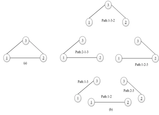
Let us consider a simple network consisting of three nodes where each node is connected to the other two nodes, i.e., the network topology looks like a triangle, see Figure 2-6. Given the node,

32 link, path, demand, demand path-flow variables, Constraints, and the objective function are defined in [64]. 3 1 2 3 1 2 3 1 2 3 1 1 2 3 2 3 1 2 (a) _Path:1-2-3 Path:2-3 Path:1-3-2 Path:2-1-3 Path:1-2 Path:1-3 (b)

Figure 2-6: (a) A three node network example (b) All possible paths for the three-node example.

2.11.1.1 Network flow example in link-path formulation

Example description:

Suppose that the demand volume between nodes 1 and 2 is 5, between nodes 1 and 3 is 7, and between nodes 2 and 3 is 8 (units), and the demand is assumed to be bi-directional.

ĥ12 = 5, ĥ13 = 7, ĥ23 = 8

The demand volume for the given network for a pair of nodes can be routed over two paths. For instance, the demand pair with end nodes 1 and 2, its demand volume is routed over the direct-link route 1-2 and the alternate route 1-3-2 via node 3 as shown in Figure 2-6-b. So, if we use 𝑥 with an

33 appropriate subscript identifier to denote the unknown demand path-flow variables, then for demand pair (1,2), we can write:

𝑥 + 𝑥 = 5 (=ĥ12)

In any communication system, the total link load must not exceed the total link capacity. Thus, we have the following inequality for link 1-2:

𝑥 + 𝑥 + 𝑥 ≤ Ĉ12

In this example, we assume that the capacity of the first two links is 10 and the third is 15 (units); thus: Ĉ12 = Ĉ13 = 10, Ĉ23 = 15

Suppose the goal of this example is to minimise the total routing cost. Assuming that the cost of routing one unit of flow on every link along its path is simply set to 1, the total routing cost for all the flow variables is:

𝑭 = 𝑥 + 2𝑥 + 𝑥 + 2𝑥 + 𝑥 + 2𝑥 Put all together:

Minimise: 𝑭 = 𝑥 + 2𝑥 + 𝑥 + 2𝑥 + 𝑥 + 2𝑥 Subject to: 𝑥 + 𝑥 = 5 𝑥 + 𝑥 = 7 + 𝑥 + 𝑥 = 8 𝑥 + 𝑥 + 𝑥 ≤ 10 𝑥 + 𝑥 + 𝑥 ≤ 10 𝑥 + 𝑥 + 𝑥 ≤ 15 𝑥 , 𝑥 , 𝑥 , 𝑥 , 𝑥 , 𝑥 ≥ 0

34 Optimal solution/optimal cost is:

𝑥 ∗ = 5, 𝑥 ∗= 7, 𝑥 ∗ = 8, 𝐹∗ _{= 20.}

2.11.2 Node-link formulation

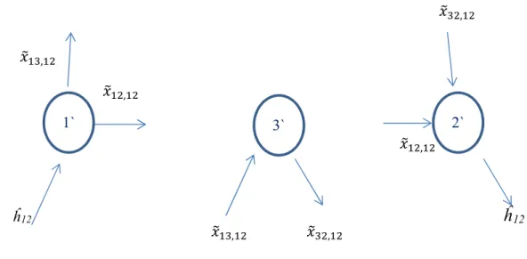
The notions of link and path was used in the mathematical formulation presented in the previous network optimisation problem example. However, there is still another way to represent the same problem. Consider directed demands on directed links and fixed demand pairs and fixed nodes. Here we considered the total link flow for a specific demand on each link, which is zero for most links. Now from the point of view of a fixed node which is not the destination or the end node of the considered demand, called transit or an intermediate node, the flows come into this node on the incoming links and go out on its outgoing links un-altered, provided the node is not the source node or the destination node of the demand. This is called flow conservation law which is described in Figure 2-7.

Figure 2-7: Demand flow view between nodes 1 and 2.  link flow: traffic of one demand on each link

 flow conservation: Source, Destination, Transit node. ĥ12 𝑥 , 𝑥 , 𝑥 , 𝑥 , 3` 𝑥 ,

ĥ

35

2.11.2.1 Optimisation in node-link formulation example

If we consider demand (1:2) and according to the flow conservation law, with the use of the convention that anything entering the node is negative and anything leaving is positive, we may write the following equation for node 1:

−ĥ12−𝑥 , − 𝑥 , + 𝑥 , + 𝑥 , = 0

It is important to consider that for each undirected link, one of its two flows is always equal to 0. This is because what really matters is the net flow on a link, which means:

ĥ12−𝑥 , − 𝑥 , + 𝑥 , + 𝑥 , = 0

Making use of the above observations we can write the set of flow conservation equations for demand (1:2) as:

𝑥 , + 𝑥 , = ĥ12 −𝑥 , + 𝑥 , = 0 −𝑥 , − 𝑥 , = −ĥ12

If we now consider the demand (1:3) from node 1 to node 3, and demand (2:3) from node 2 to node 3, we obtain the following equalities:

𝑥 , + 𝑥 , = ĥ13 −𝑥 , + 𝑥 , = 0 −𝑥 , − 𝑥 , = − ĥ13 𝑥 , + 𝑥 , = ĥ23 −𝑥 , + 𝑥 , = 0 −𝑥 , + 𝑥 , = −ĥ23