The University of Adelaide
School of Economics
Research Paper No. 2010-09
May 2010
Estimation in Single-Index Panel Data Models
with Heterogeneous Link Functions
Estimation in Single–Index Panel Data Models
with Heterogeneous Link Functions
By Jia Chen, Jiti Gao and Degui Li
School of Economics, The University of Adelaide, Adelaide, Australia
Abstract
In this paper, we study semiparametric estimation for a single–index panel data model where the nonlinear link function varies among the individuals. We propose using the so–called refined minimum average variance estimation based on a local linear smoothing method to estimate both the parameters in the single–index and the average link function. As the cross–section dimension N and the time series dimensionT tend to infinity simultaneously, we establish asymptotic distributions for the proposed parametric and nonparametric estimates. In addition, we provide two real–data examples to illustrate the finite sample behavior of the proposed estimation method in this paper.
Keywords: Asymptotic distribution, local linear smoother, minimum average variance estimation, panel data, semiparametric estimation, single–index models.
1. Introduction
During the last two decades or so, there exists a huge literature on parametric lin-ear and nonlinlin-ear panel data modeling as the double–index models enable reslin-earchers to extract information that may be difficult to obtain through purely cross–section or time–series data models. We refer to the books by Baltagi (1995), Arellano (2003) and Hsiao (2003) for an overview of statistical inference and econometric analysis of parametric panel data models. As in both the cross–section and time–series analy-sis, however, parametric models may be misspecified and estimators obtained from such misspecified parametric models are often inconsistent. To address such issues, some nonparametric and semiparametric models have been proposed, see Li and Sten-gos (1996), Ullah and Roy (1998), Abrevaya (1999), Hjellvik, Chen and Tjøstheim (2004), Cai and Li (2008), Henderson, Carroll and Li (2008) and Mammen, Støve and Tjøstheim (2009) for example.
There is a growing interest in using single–index models in both the cross–sectional and time series cases (see, for example, H¨ardle, Hall and Ichimura 1993; Carroll et al. 1997; Xia et al. 2002; Yu and Ruppert 2002; Xia 2006; Gao 2007). So far as we know, however, there is little study in the theoretical and empirical analysis of single– index models for panel data. Single–index models search for a linear combination of the multi–dimensional covariate{Xit}which can capture most information about the relationship between the response variable{Yit}and covariate{Xit}. For a real data, there may exist individual effects. For example, in the US cigarette demand data set given in Section 5, there are state-specific effects such as religion, race, education and tourism. To reflect the individual effects, we assume that the nonlinear link function g(·) varies across the individuals. The model we study in this paper is given as follows: Yit =gi(θ0>Xit) +εit, 1≤i≤N, 1≤t≤T, (1.1) whereg(·) is an unknown link function andθ0 is ap×1 vector of unknown parameters.
For identifiability, we requirekθ0k= 1 throughout the paper.
This paper is interested in the case that the cross–section dimension N and the time–series dimensionT tend to infinity simultaneously. Model (1.1) is call a single– index panel data model with heterogeneous link functions and it is more flexible than a homogeneous single–index panel data model. In this paper, we assume that
{Xit, εit, t ≥ 1} is stationary α–mixing for each i. It is well–known that α–mixing dependence is one of the weakest mixing conditions for weakly dependent processes and it can be satisfied for some stationary time series and Markov chains under certain conditions. This means that we can apply model (1.1) to the dynamic panel data case, which will be discussed in Section 4.
In Section 2, we extend the so–called refined minimum average (conditional) vari-ance estimation (RMAVE) method for the time series case to estimate the parameter θ0in model (1.1). The RMAVE was introduced by Xia et al. (2002) and its asymptotic
distribution was established by Xia (2006) in the time series case. As there are two indices involved in our case and the nonlinear link functions are heterogeneous, the establishment of our asymptotic theory is much more complicated than that for the time series case. We show, in Section 3, that under certain regularity conditions, the RMAVE ofθ0 is asymptotically normal with
√
N T rate of convergence asN, T → ∞ simultaneously. This is called the joint limiting distribution (see Phillips and Moon 1999 for detail). Meanwhile, since the link functionsgi(·) vary across the sections, it is reasonable to study a nonparametric estimate of the average link function of the form g(x) = 1 N N X i=1 gi(x). (1.2)
In Section 3, we also establish an asymptotic distribution for the local linear estimate of g(x).
When {Xit} contains lagged values of Yit, (1.1) becomes a dynamic panel data model. Section 4 discusses some conditions that ensure{Yit, t≥1}to be a geometri-cally ergodic time series for eachi. In this case, the stationarity and mixing conditions and thus the asymptotic properties in Section 3 still hold for such a dynamic model. We include two empirical examples in Section 5 to illustrates the applicability of the proposed models and estimation method. One is the US cigarette demand data for 46 states from 1963 to 1992, to which we fit a single index model whose covariates Xit contain a lagged value ofYit. We compare our RMAVE results with the ordinary least squares (OLS) estimation results for a linear panel data model from Baltagi, Griffin and Xiong (2000), and find that our estimated covariate coefficients are more significant than the OLS estimates. We then discuss an empirical application to a climatic date set from the UK by examining the relationship between the monthly
average maximum temperatures and the number of millimeters of rainfall and hours of sunshine duration. The heterogenous link functions used allow us to take into account the state or station specific effects.
The rest of the paper is organized as follows. In Section 2, we develop the de-tailed algorithm of a RMAVE method. Section 3 establishes the asymptotic theory for both the parameter estimator and nonparametric estimate. Section 4 discusses the conditions for a dynamic single-index model to be geometrically ergodic, which ensures that the asymptotic properties in Section 3 are still valid for the dynamic model. Sections 5 includes a brief discuss on the bandwidth selection problem and two real data exmples. Section 6 concludes this paper. Some technical lemmas and the detailed proofs of the main results are given in Appendices A and B.
2. Semiparametric estimation method
In this section, we develop a RMAVE method to estimate both the parameter θ0
in the single–index and the averaged link function defined in Section one. As the link functions are heterogeneous, the RMAVE method originally studied in Xia (2006) for the time series case will need to be extended substantially to deal with our case.
Given θ>Xit=u, define σθ,i2 (u) =E Yit−gi(θ>Xit) 2 |θ>Xit =u (2.1) for 1≤i≤N. Note that
EYit−gi(θ>Xit)
2
=Eu
h
σ2θ,i(u)i. (2.2) Based on (2.1) and (2.2), the estimator of θ0 can be obtained by minimizing
N X i=1 EYit−gi(θ>Xit) 2 = N X i=1 Eu h σθ,i2 (u)i.
As the link functions gi(·) are unknown for the single–index panel data case, we estimate them by the local linear method. It is well–known that the local linear fitting has advantages over the Nadaraya–Watson kernel method, such as high asymptotic efficiency, design adaption and automatic boundary correction (see Fan and Gijbels 1996 for example). ForXit close to the pointx, by Taylor expansion, we have
Yit−gi(θ>Xit) = Yit−gi(θ>x)−gi0(θ
>
Letθb1 be an initial estimator ofθ0. Based on the above local linear approximation,
we describe the detailed algorithm as follows. Step 1. Let θ =θb1. Calculate
ais bis = 1 T T X t=1 Kh(θ>Xits) 1 θ>Xits 1 θ>Xits > −1 × 1 T T X t=1 Kh(θ>Xits) 1 θ>Xits Yit , (2.3)
wherehis a bandwidth,K(·) is a kernel function, Kh(·) = 1hK(·/h), andXits= Xit−Xis. Step 2. Obtain e θ = (N X i=1 T X t=1 T X s=1
Kh(θ>Xits)bis2XitsXits>/fb θ i(θ > Xis) )+ × (N X i=1 T X t=1 T X s=1 Kh(θ>Xits)bisXits(Yit−ais)/fbθ i(θ > Xis) ) , (2.4) where fbθ,i(θ>Xis) = 1 T T P t=1
Kh(θ>Xits), θ =θb1, and A+ stands for the
pseudoin-verse of A.
Step 3. Update θ with θ =θ/e kθek. Repeat Step 1 and Step 2 until convergence.
We denote the final estimate byθ. In order to implement the above algorithm, web
need to choose a suitable initial estimator of θ0 and an optimal bandwidth h. Such
issues will be discussed in Sections 3 and 4 below.
Let gbi(x) =ai,x, whereai,x is defined as ais in (2.3) with θ and Xis replaced by θb
and x, respectively. As in Hjellvik, Chen and Tjøstheim (2004), the nonparametric estimate of g(x) is defined as b g(x) = 1 N N X i=1 b gi(x).
An asymptotic distribution of g(x), asb T, N → ∞ simultaneously, is established
3. Asymptotic theory
In this section, we establish asymptotic distributions for θb and b
g(·). Before giv-ing some regularity assumptions, we introduce followgiv-ing notation. Define µθ,i(u) = E(Xit|θ>Xit = u) and νθ,i(x) = µθi(θ
>x)−x. We then introduce the following
as-sumptions.
A1. K(·) is a symmetric and continuous kernel function with some bounded support, and its derivative is bounded. Furthermore, R
K(u)du= 1.
A2 (i). LetXi ={Xit, t≥1} and εi ={εit, t≥1}. Suppose that {Xi, εi},i≥1, are independent.
(ii). For eachi,{(Xit, εit), t≥1}is a stationary sequence of α–mixing random vectors with E(εit|θ>Xit) = 0, max
i E h |εit|2+δ i < ∞, max i E h kXitk2+δ i < ∞ and mixing coefficient αi(·) satisfying max
i αi(t) =O(t
−κ) for κ > (2+δ)
δ .
A3(i). Letfθ,i(·) be the density function of {θ>Xit, t≥1}. Suppose thatfθ,i(·) is continuous and its derivatives of up to the third order are bounded. Uniformly for θ in a neighborhood of θ0, min i kxk≤infCN T fθ,i(θ>x)>0, whereCN T =C(N T) 1 2+δ for some C > 0.
(ii). For 1≤ i≤N, each of the link functions gi(·) has bounded derivatives of up to the third order.
(iii). µθ,i(·) is continuous and has bounded derivatives of up to the second order. A4. The bandwidthhsatisfiesN T h→ ∞,N T h6 →0,α
T ,h/h→0,N T α2T,hh2 →0, αT ,h(N T)1/(2+δ) → 0 and (N T)1+(p+κ+2)/(2+δ)α κ−p T ,hh−1−p → 0, where αT,h = q logT
T h and κ is as defined in A2(ii) above.
Remark 3.1. A1 is a set of some mild conditions on the kernel function, which have been used by many authors in the time series case (see Fan and Yao 2003; Gao 2007 for example). In A2, we assume that (Xi, εi),i≥1, are cross–sectional independence (see Cai and Li 2008 for example) and each time series isα–mixing, which can be satisfied
by many linear and nonlinear time series models (see, for example, Auestad and Tjøstheim 1990, Chen and Tsay 1993 for example). A3 is about some commonly–used conditions in single–index models (see Xia 2006 for example). In A4, the condition αT ,h/h→ 0 impliesT h3 → ∞. On the other hand, N T α2T,hh2 → 0 impliesN h →0. Therefore, T h−3 N3, which indicates that the limiting theory in this paper
holds under the condition that the rate of T tending to infinity is faster than that of N3. This is a rigorous condition and is due to the fact that we use individual time
series to estimate the individual–specific link functions gi(·) (1≤i≤N) and use the pooled data to estimate the index parameter θ0.
Note that (N T)1+(p+κ+2)/(2+δ)ακ−p T ,h h
−1−p → 0 is close to α
T,h(N T)1/(2+δ) → 0 as κ → ∞. In addition, if δ → ∞, αT ,h(N T)1/(2+δ) → 0 is close to αT ,h → 0, which is a conventional condition for uniform consistency of nonparametric kernel–based statistics in the time series case. When T ∼ N4 and h ∼ (N T)−θ, it can be shown that N T h → ∞, N T h6 → 0, α
T,h/h → 0 and N T αT,h2 h2 → 0 are all satisfied when
1
6 < θ < 1 5.
Before stating an asymptotic distribution for θbdefined in Section 2, we introduce
some notation. LetWit =
Xit−µθ0,i(θ
>
0Xit)
g0i(θ>0Xit)εit. By A2 (ii), we know that for each i, Λi,T := 1 TVar " T X t=1 Wit # =EhWi1Wi>1 i + 2 T X t=2 1− (t−1) T ! EhWi1Wit> i <∞. Let Dθ0,i =E g0i(θ>0Xis) 2 νθ0,i(Xis)ν > θ0,i(Xis) .
In order to establish the asymptotic normality of θ, we need to assume that thereb
is an initial estimatorθb1such thatkθb1−θ0k=OP
(N T)−1/2. The proof of Theorem
3.1 below is given in Appendix B.
Theorem 3.1. Assume that conditions A1–A4 hold and that there exist two positive definite matrices Σθ0 and Dθ0 such that
1 N N X i=1 Λi,T →Σθ0 (3.1) as N, T → ∞ simultaneously and 1 N N X i=1 Dθ0,i→Dθ0 as N → ∞. (3.2)
Additionally, as N, T → ∞ simultaneously 1 N max 1≤i≤NΛi,T →0. (3.3)
If the initial estimator θb1 is
√
N T–consistent, then we have √ N T θb−θ0 d −→N(0, D+θ 0Σθ0D +> θ0 ) (3.4) as N, T → ∞ simultaneously, where D+θ 0 is the pseudoinverse of Dθ0.
Remark 3.2. The above theorem shows that the estimatorθbis asymptotically normal
with √N T rate of convergence even when the link functions may be heterogeneous. Equations (3.1) and (3.3) are imposed to make sure that the Lindeberg condition holds when we prove the joint central limit theorem. In the meantime, the condition that the initial estimate is √N T–consistent is similar to the √T–consistency condition in the one–index case (see H¨ardle, Hall and Ichimura 1993 and Carroll et al 1997 for example). As a matter of the fact, this restriction is feasible as such an initial estimator can be obtained by using some existing methods (see, for example, H¨ardle and Stoker 1989; Horowitz and H¨ardle 1996).
Let bg,i(u) = 12µ2gi00(u) and σ2i(u) = ν0σθ20,i(u)/fθ0,i(u), where µk =
R ukK(u)du, νk = R ukK2(u)du andσ2 θ0,i(u) = E ε2 it|θ > 0Xit=u
. We next establish an asymptotic distribution forg(x) in the following theorem; its proof is given in Appendix B.b
Theorem 3.2. Assume that the conditions of Theorem 3.1 are satisfied. If, in addi-tion, N T h4 → ∞, 1 N N X i=1
bg,i(u)→bg(u), 1 N N X i=1 σi2(u)→σ2g(u) as N → ∞, (3.5) and max 1≤i≤Nσ 2 i(u) =o(N), then, as N, T → ∞ simultaneously, √
N T hg(u)b −g(u)−bg(u)h
2−→d N0, σ2
g(u)
. (3.6)
Remark 3.3. Note that Theorem 3.2 covers the case that g(·) can be consistently estimated by g(b ·) when model (1.1) reduces to the case where the link functions are
4. Dynamic single-index panel data models
We next consider the case that Xit contains lagged values ofYit. If Xit =Yei,t−1 =
(Yi,t−1,· · ·, Yi,t−p)
>
, then model (1.1) becomes Yit =gi
θ0>Yei,t−1
+εit, (4.1)
where, for each i, {it, t ≥ 1} is a sequence of i.i.d. random variables and εit is independent of Yi,s for all s < t. To ensure that the asymptotic distributions in Section 3 still hold for this dynamic model, we provide some sufficient conditions for {Yit, t≥1}to be geometrically ergodic for eachi≥1. This implies that{Yit, t≥1} satisfies the stationarity and mixing conditions. Motivated by Theorems 3.1 and 3.2 in An and Huang (1996), we give two kinds of conditions on the link functionsgi that ensure the geometrical ergodicity of {Yit, t≥1}.
Proposition 4.1.Let φi(x1,· · ·, xp) =gi(θ>x) with x= (x1,· · ·, xp)>. (i). Suppose that
sup
kxk≤C
|φi(x)|<∞ for any C > 0 and i≥1 (4.2)
lim kxk→∞ φi(x)−α > i x kxk = 0 for each i≥1, (4.3) where αi = (αi,1,· · ·, αi,p) > satisfies
xp−αi,1xp−1− · · · −αi,p−1x−αi,p 6= 0 for all |x|>1. (4.4) Then, {Yit, t ≥1} defined by (4.1) is geometrically ergodic for each i≥1.
(ii). Suppose that there exists a positive number λi <1 and a constantCi for each i, such that
|φi(x)| ≤λimax{|x1|,· · ·,|xp|}+Ci. (4.5) Then {Yit, t ≥1} defined by (4.1) is geometrically ergodic for each i≥1.
The detailed proof of Proposition 4.1 follows from the same arguments as used in An and Huang (1996). Similar results about geometrical ergodicity are available from Masry and Tjøstheim (1995), and Lu (1998).
Example 4.1. Let θ0 = (θ01, θ02)
>
= (0.6,0.8)> and gi(u) = √12u+ sin(2iπu). Then the dynamic panel data model (4.1) reduces to
Yit = 1 √
2(0.6Yi,t−1 + 0.8Yi,t−2) + sin
2π(0.6Yi,t−1+ 0.8Yi,t−2)
i
!
+εit.
As sin(·) is a bounded function, by letting αi =
0.6 √ 2, 0.8 √ 2 > , it is easy to show that (4.2) and (4.3) are satisfied. Hence, by Proposition 4.1 (i), {Yit, t ≥ 1} is geometrically ergodic for each i≥1.
Example 4.2. Assume that the link functions gi(·) satisfy |gi(u)| ≤
ρi|u| √
p +κi, for any u∈R,
where κi and ρi are positive constants, ρi <1, and p is the dimension of θ0 in (4.1).
Following the same arguments as used in Example 3.5 of An and Huang (1996), we can show that (4.5) holds with λi = ρi and Ci = κi. And hence, {Yit, t ≥ 1} is geometrically ergodic for each i≥1. On the other hand, ifgi(·) satisfies
lim
|u|→∞
|gi(u)−c∗iu|
|u| = 0, for each i≥1,
wherec∗i satisfies (4.4) in Proposition 4.1 (ii), then we also can show that{Yit, t≥1} is geometrically ergodic for each i≥1.
5. Empirical examples
We give a brief discussion on the bandwidth selection and then give two real data examples to illustrate the proposed estimation method.
5.1. Bandwidth selection
Bandwidth selection is important for nonparametric estimation. Consider the es-timate ofg at the final step of the iterations. It follows from (3.6) that the asymptotic integrated mean squared error of g(b ·) is given by
h4 Z b2g(u)du+ R σ2g(u)du N T h and an optimal global bandwidth is of the form
hopt = R σ2 g(u)du 4R b2 g(u)du (N T)−1/5. (5.1)
Based on (5.1), we can use the plug–in method (see Ruppert, Sheather and Wand 1995 for detail) to choose an optimal bandwidth for the implementation of (5.1) in practice. In the real data application below, we instead propose using a semipara-metric leave-one-out cross validation method to select the bandwidth.
Suppose that θ(h) is an estimate ofb θ0 via the iterative procedure described in
Section 2 with bandwidth h. For each 1≤i≤N and 1≤t≤T, we calculate a(it−t)(h) = T X s=1,s6=t Kh b θ(h)>Xits −1 T X s=1,s6=t Kh b θ(h)>Xits Yis , (5.2) and let CV(h) = 1 N T N X i=1 T X t=1 Yit−a (−t) it (h) 2 . (5.3)
Then, we choose hb = arg min
h CV(h) as an optimal bandwidth in our implemen-tation in the rest of this section.
5.2. Real data examples
Example 5.1. The first example is about the cigarettes demand in 46 American states over the period 1963–1992. The data set is from Baltagi, Griffin and Xiong (2000). The data set contains 7 variables: average retail price per pack of cigarettes, population, population above the age of 16, consumer price indices, real per capita dis-posable income, real per capita sales of cigarettes and minimum real price of cigarettes in any neighboring state.
As in Baltagi, Griffin and Xiong (2000) and Mammen, Støve and Tjøstheim (2009), we use only four variables to model cigarettes demand: real per capita sales of cigarettes (denoted as Yi,t), average retail price per pack of cigarettes (denoted as Xi,t,2), real per capita disposable income (denoted as Xi,t,3) and minimum real price
of cigarettes in any neighboring state (denoted asXi,t,4). DenoteXi,t,1 =Yi,t−1,i= 1,
· · ·, 46, t = 1, · · ·, 29. Baltagi, Griffin and Xiong (2000) modeled the data with the following log-linear dynamic demand model
lnYi,t =α+β1lnXi,t,1+β2lnXi,t,2+β3lnXi,t,3+β4lnXi,t,4+ui,t, (5.4) where ui,t = µi +λt+vi,t, µi denotes a state-specific effect, and λt denotes a year-specific effect. In this paper, we use a single–index panel data model with heteroge-neous link functions. By allowing the link functions to vary across states, we can also
incorporate state-specific effects such as religion, race, tourism, tax, and education into our model.
As all the four variables exhibit a time trend, we first remove the trend from the data. Similarly to Mammen, Støve and Tjøstheim (2009), we make the following transformation
e
Yi,t = lnYi,t−sY(t) and Xfi,t,l = lnXi,t,l−sX
l(t), l = 1,· · ·,4,
where sY(t) is the nonparametric estimator of the time trend in observations lnYi,t, and sXl(t) is the nonparametric estimator of the trend in observations lnXi,t,l. sY(t) can also be seen as time-specific effects λt in model (5.4), which may include policy interventions, health warnings and so on. We then assume that
e
Yi,t =gi(θ>Xfi,t) +εi,t, i= 1,· · ·,46, t= 1,· · ·,29, (5.5)
where Xfi,t =
f
Xi,t,1,Xfi,t,2,Xfi,t,3,Xfi,t,4 >
, and θ = (θ1, θ2, θ3, θ4)> is the vector of
parameters to be estimated. We apply the RMAVE estimation method proposed in Section 2 to the transformed observations. For the initial estimator θb1 of θ, we
use a normalized version of Baltagi, Griffin and Xiong (2000)’s OLS estimate of β = (β1, β2, β3, β4)> from model (5.4): θb1 = bβ
kbβk
= (0.9765,−0.2029,0.0456,0.0575)>. Our semiparametric estimate of θ is then θb= (0.9171,−0.3478,0.1764,0.0823)>.
Comparison of our estimate with Baltagi, Griffin and Xiong (2000)’s OLS estimate sees a drop in the coefficient for the lagged consumption from 0.9765 to 0.9171, and increases in all the other covariate coefficients, especially in the coefficient for disposable income (Xi,t,3) which sees almost a threefold increase from 0.0456 to 0.1764.
Mammen, Støve and Tjøstheim (2009) used a nonparametric additive model to fit the data and found a similar result: the nonparametric estimates of the elasticities for retail price, disposable income, and minimum price in any neighboring state (Xi,t,2,
Xi,t,3, and Xi,t,4) are more significant than Baltagi, Griffin and Xiong (2000)’s OLS
estimates.
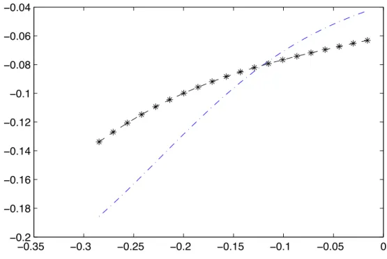
To see whether the estimates of the link functions vary across states, we plotted the estimated link functions for the first two states in Figure 5.1. The figure shows that there does exist some level of difference between the nonparametric estimates of the link functions for the two states.
!0.35 !0.3 !0.25 !0.2 !0.15 !0.1 !0.05 0 !0.2 !0.18 !0.16 !0.14 !0.12 !0.1 !0.08 !0.06 !0.04
Figure 5.1. Estimated link functions for the first (dash-dotted line) and second (dash-starred line) states.
Example 5.2. The second data set, which is available from the UK Met Office website http://www.metoffice.gov.uk/climate/uk/stationdata/, contains monthly data of the average maximum temperature (TMAX), the average minimum temperature (TMIN), the number of days of air frost (AF), the number of millimeters of rainfall (RAIN), and the number of hours of sunshine (SUN). The data were collected from 37 stations across the UK. We select data over the decade of January 1999–December 2008 from 16 stations according to data availability.
Both seasonality and trend are first removed from the data and we focus on investigating the relationship between the TMAX and RAIN and SUN. For thei–th station, denote the seasonality and trend removed TMAX at time t as Yi,t, and the seasonality and trend removed RAIN and SUN as Xi,t,1 and Xi,t,2, respectively. We
then use the proposed semiparametric RMAVE method to estimate the parameter θ in the model
Yi,t =gi(θ>Xi,t) +εi,t, i= 1,· · ·,16, t= 1,· · ·,120, (5.6) where Xit = (Xi,t,1, Xi,t,2)
>
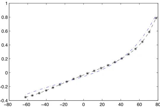
!80 !60 !40 !20 0 20 40 60 80 !0.4 !0.2 0 0.2 0.4 0.6 0.8 1
Figure 5.2. Estimated link functions for stations Armagh dotted line) and Bradford (dash-starred line).
estimate β in a linear model of the form
Yi,t =Xi,t>β+αi+ei,t, (5.7) whereαi are station-specific effects. Then, we use the normalized LS estimate kβb
b
βk =
(0.1931,0.9812)> as the initial estimate forθ in the RMAVE estimation of (5.6). The resulting RMAVE estimator of θ is θb = (0.1046,0.9945)>, which sees a drop from
0.1931 to 0.1046 in the coefficient for the rainfall covariate and a slight increase in the coefficient of sunshine.
As in Example 5.1, plots of the link functions for the first two stations are given in Figure 5.2. The figure shows the two estimated functions almost coincide which indicates that the difference between the two link functions is small.
6. Conclusion
We have considered an estimation problem in a single–index panel data model with heterogeneous link functions. A nonparametric local linear based minimum average variance estimation method has been proposed to estimate the parameter vector and
an average of the link functions. An asymptotically normal distribution has been established for each of the proposed estimates. In addition, we have included two real data examples to show how the proposed theory and estimation method is illustrated and implemented in practice.
The paper has some limitations and several extensions may be done. One of the topics is to establish some corresponding theory for the case where the residuals are cross–sectionally dependent. Another of the topics is whether the established theory may be extended to the case where{Xit} is nonstationary in t and cross–sectionally dependent in i. Such topics may be discussed in future research.
7. Acknowledgments
The authors would like to acknowledge the financial support from the Australian Research Council Discovery Grants Program under Grant Number: DP0879088. Thanks also go to Dr B˚ard Støve for providing us with the data set used in Ex-ample 5.1.
Appendix A: Technical lemmas
Let Xit,x=Xit−x. We assume without loss of generality that µ2 = 1 (otherwise, we
can letK(u) =µ21/2K(µ12/2u)). Denote ΘN T = n θ: |θ−θ0| ≤Cθ(N T)−1/2 o , XN T =nx:kxk ≤M(N T)1/(2+δ)o, and FN T ={(x, θ) : x∈ XN T, θ∈ΘN T},
whereCθ and M are two positive constants. Define
Zh(x, Xit) =Kh(θ>Xit,x) θ>Xit,x h !k Xit,x and Zh∗(x, Xit) =Kh(θ>Xit,x) θ>Xit,x h !k .
Lemma A.1.Let A1, A2, A3 (i)(iii) hold. If, in addition,
h→0, (N T)1/(2+δ)αT,h →0, (N T)1+(p+κ+2)/(2+δ)ακ
−p T ,hh
we have max 1≤i≤Nx∈Xsup N T 1 T T X t=1 Zh∗(x, Xit)−fθ,i(θ>x)µk−fθ,i0 (θ > x)µk+1h =OP(h2+αT ,h) (A.1) and max 1≤i≤Nx∈XsupN T 1 T T X t=1 Zh(x, Xit)−fθ,i(θ>x)νθ,i(x)µk− h fθ,i(θ>x)µθ,i(θ>x) i0 µk+1h = OP(h2+αT ,h), (A.2)
where fθ,i0 (θ>x) is the derivative of fθ,i(θ>x).
Proof. We only prove (A.2) as the proof of (A.1) is similar. To prove (A.2), we first prove
max 1≤i≤Nx∈XsupN T 1 T T X t=1 (Zh(x, Xit)−E[Zh(x, Xit)]) =OP(αT ,h). (A.3)
We first partition the set XN T into B balls Bk, 1 ≤ k ≤ B, each centered at xk with
radiusr=O(hαT ,h). By a simple calculation, we have B=O(N T)p/(2+δ)h−pα−T ,hp.
Then, for eachθ∈ΘN T we have
max 1≤i≤Nx∈Xsup N T 1 T T X t=1 (Zh(x, Xit)−E[Zh(x, Xit)]) ≤ max 1≤k≤B1max≤i≤N 1 T T X t=1 (Zh(xk, Xit)−E[Zh(xk, Xit)]) + max 1≤k≤Bxsup∈B k max 1≤i≤N 1 T T X t=1 ([Zh(x, Xit)−Zh(xk, Xit)]−E[Zh(x, Xit)−Zh(xk, Xit)]) =: max
1≤k≤B1max≤i≤N|HT ,1(k, i)|+ max1≤k≤Bxsup∈B
k
max
1≤i≤N|HT ,2(k, i, x)|. (A.4)
We first consider max
1≤k≤B1max≤i≤NHT ,1(k, i). Let
Zh(xk, Xit) =Zh(xk, Xit)I{kXitk ≤∆N T},
Zhc(xk, Xit) =Zh(xk, Xit)−Zh(xk, Xit),
where ∆N T = (N T)1/(2+δ)L(N T), andL(·) is a positive slowly–varying function satisfying
L(N T)→ ∞, (N T)1/(2+δ)L(N T)αT,h →0,
(N T)1+(p+κ+2)/(2+δ)αT ,hκ−ph−1−pLκ+2(N T)→0, (A.5) asN, T → ∞.
It is easy to check that HT,1(k, i) = 1 T T X t=1 n Zh(xk, Xit)−E h Zh(xk, Xit) io +1 T T X t=1 {Zhc(xk, Xit)−E[Zhc(xk, Xit)]}.
By the first term in (A.5) and EhkXitk2+δ
i
<∞ in A2(ii), we can show that for any
η >0, P max 1≤k≤B1max≤i≤N 1 T T X t=1 {Zhc(xk, Xit)−E[Zhc(xk, Xit)]} > ηαT ,h ! ≤ N X i=1 T X t=1 EkXitk2+δ N T L2+δ(N T) ≤ 1 L2+δ(N T) =o(1),
which implies that max 1≤k≤B1max≤i≤N 1 T T X t=1 {Zhc(xk, Xit)−E[Zhc(xk, Xit)]} =OP(αT ,h). (A.6)
Furthermore, by A1, A2(ii), A3(i) and the standard argument for the variance of α– mixing nonparametric kernel statistic, we have
max 1≤k≤B1max≤i≤NVar T X t=1 Zh(xk, Xit) ! =OT h−1. (A.7) Then, by Bernstein inequality forα–mixing processes (see Theorem 2.18 in Fan and Yao 2003 for example), P 1 T T X t=1 n Zh(xk, Xit)−EZh(xk, Xit) o > ηαT ,h ! = P T X t=1 n Zh(xk, Xit)−EZh(xk, Xit) o > ηT αT ,h ! ≤ 4 exp−Cη2logT+CT ακT h∆κN T+2h−1,
whereC is some positive constant. Hence, as N T ακT h−ph−p =o(1),
P max 1≤k≤B1max≤i≤N 1 T T X t=1 {Zh(xk, Xit)−EZh(xk, Xit)} > ηαT,h ! ≤ OBN T−Cη2+BN T ακT h∆κN T+2h−1 = Oα−T,hph−pN1+p/(2+δ)Tp/(2+δ)−Cη2 + (N T)1+(p+κ+2)/(2+δ)αT hκ−ph−1−pLκ+2(N T) = o(1)
when η is large enough, which, together with (A.6), implies max
Meanwhile, by A1 we have max 1≤k≤Bxsup∈B k max 1≤i≤N|Zh(x, Xit)−Zh(xk, Xit)| ≤ Ch−1 max 1≤k≤Bxsup∈B k |x−xk| ! ≤Ch−1hαT ,h =O(αT ,h), which implies max 1≤k≤Bxsup∈B k max 1≤i≤NHT,2(k, i, x) =OP(αT,h). (A.9)
Combining (A.4), (A.8), (A.9) and the proof of Lemma 6.7 in Xia (2006), we obtain (A.3).
Moreover, by A1 and A3 (i)(iii), we obtain
E Kh(θ>Xit,x) θ>Xit,x h !k =fθ,i(θ>x)µk+fθ,i(θ>x)µk+1h+O(h2), and E Kh(θ>Xit,x) θ>Xit,x h !k Xit,x =fθ,i(θ>x)νθ,i(x)µk+ h fθ,i(θ>x)µθ,i(θ>x) i0 µk+1h+O(h2).
Lemma A.1 follows immediately from (A.3) and the above two equations.
Lemma A.2. Letting ai,x and bi,x be defined as ais and bis with Xits replaced by Xit,x in (2.3), then under A1–A3,
ai,x = gi(θ>0x) +g 0 i(θ > 0x)(θ0−θ)>νθ,i(x) + 1 2g 00 i(θ > 0x)h2+ 1 T fθ,i(θ>x) T X t=1 Kh(θ>Xit,x)εit +O|δθ|2+h(h2+αT ,h) +α2T ,h+ (h+αT,h)|δθ| (A.10) and bi,x = g0i(θ > 0x) + 1 T hfiθ(θ>x) T X t=1 Kh(θ>Xit,x) θ>Xit,x h ! εit (A.11) + Oh2+αT ,h+α2T ,h/h+ (h+αT ,h)|δθ|/h+|δθ|2/h ,
uniformly hold for x∈ XN T, where δθ =θ−θ0.
Proof. DefineSi,kθ = T1
T
P
t=1
Kh(θ>Xit,x)(θ>Xit,x)k fork= 0, 1, 2, 3. By simple calculation,
we have ai,x= Si,θ0Si,θ2−Si,θ12 −1(1 T T X t=1 Kh(θ>Xit,x) Si,θ2−Si,θ1(θ>Xit,x) Yit ) (A.12)
and bi,x = Si,θ0Si,θ2−Si,θ12 −1(1 T T X t=1 Kh(θ>Xit,x) Si,θ0(θ>Xit,x)−Si,θ1 Yit ) . (A.13) By Lemma A.1, we have uniformly for x∈ XN T,
Si,θ0 =fθ,i(θ>x) +OP(h2+αT ,h), (A.14) Si,θ1 =OP(h(h+αT ,h)) =OP(h2+hαT ,h), (A.15) Si,θ2 =fθ,i(θ>x)h2+OP h2(h2+αT ,h) , (A.16) Si,θ3 =OP(h3(h+αT ,h)) =OP(h4+h3αT ,h). (A.17) Hence, by (A.14)–(A.16), Si,θ0Si,θ2−Si,θ12 =fθ,i(θ>x) 2 h2+OP h2(h2+αT ,h) . (A.18) By Taylor expansion, we have
Yit = gi(θ0>Xit) +εit = εit+gi(θ0>x) +g 0 i(θ > 0x)θ > 0Xit,x+ 1 2g 00 i(θ > 0x)(θ > 0Xit,x)2+O(|θ0>Xit,x|3) = εit+gi(θ0>x) +gi0(θ0>x)θ>Xit,x+ 1 2g 00 i(θ0>x)(θ>Xit,x)2 +gi0(θ0>x)(θ0−θ)>Xit,x+ 1 2g 00 i(θ0>x) h (θ>0Xit,x)2−(θ>Xit,x)2 i (A.19) +O|θ0>Xit,x|3 = εit+gi(θ0>x) +g 0 i(θ > 0x)θ > Xit,x+ 1 2g 00 i(θ > 0x)(θ > Xit,x)2 +gi0(θ0>x)(θ0−θ)>Xit,x+ ∆it,x, where ∆it,x = O h (θ>0Xit,x)2−(θ>Xit,x)2 i +|θ>0Xit,x|3 = O h (θ0−θ)>Xit,x i2
+ 2θ>Xit,x(θ0−θ)>Xit,x+ (θ>Xit,x)3
+ h(θ0−θ)>Xit,x i3 + 3(θ0−θ)>Xit,x(θ>Xit,x)2+ 3 h (θ0−θ)>Xit,x i2 θ>Xit,x
= O|δθ|2|Xit,x|2+|δθ||Xit,x||θ>Xit,x|+|θ>Xit,x|3+|δθ|3|Xit,x|3
+ |δθ||Xit,x||θ>Xit,x|2+|δθ|2|Xit,x|2|θ>Xit,x|
. (A.20)
Meanwhile, by (A.14)–(A.18) we have
Si,θ0Si,θ2−Si,θ12 −1(1 T T X t=1 Kh(θ>Xit,x) Si,θ2−Si,θ1(θ>Xit,x) gi(θ0>x) ) = gi(θ0>x) Si,θ0Si,θ2−(Si,θ1)2−1Si,θ0Si,θ2−(Si,θ1)2=gi(θ0>x), (A.21)
Si,θ0Si,θ2−Si,θ12 −1(1 T T X t=1 Kh(θ>Xit,x) Si,θ2−Si,θ1(θ>Xit,x) gi0(θ0>x)θ>Xit,x ) = g0i(θ>0x) Si,θ0Si,θ2−Si,θ12 −1 Si,θ1Si,θ2−Si,θ1Si,θ2= 0 (A.22) and Si,θ0Si,θ2−Si,θ12 −1(1 T T X t=1 Kh(θ>Xit,x) Si,θ2−Si,θ1(θ>Xit,x) 1 2g 00 i(θ>0x)(θ>Xit,x)2 ) = 1 2g 00 i(θ > 0x) Si,θ0Si,θ2−Si,θ12 −1 (Si,θ2)2−Si,θ1Si,θ3 (A.23) = 1 2g 00 i(θ > 0x)h2+OP h2(h2+αT ,h) . LetQθi,k = T1 T P t=1
Kh(θ>Xit,x)(θ>Xit,x)kXit,x fork= 0, 1, 2. By Lemma A.1, we have
Qθi,0=fθ,i(θ>x)νθ,i(x) +OP(h2+αT,h), (A.24)
Qθi,1=OP(h(h+αT ,h)). (A.25) As a result, we have Si,θ0Si,θ2−Si,θ12 −1(1 T T X t=1 Kh(θ>Xit,x) Si,θ2−Si,θ1(θ>Xit,x) g0i(θ>0x)(θ0−θ)>Xit,x ) = gi0(θ0>x)(θ0−θ)> Si,θ0Si,θ2−Si,θ12 −1 n Si,θ2Qθi,0−Si,θ1Qθi,1o (A.26) = gi0(θ0>x)(θ0−θ)>νθ,i(x) +OP (h2+αT ,h)|δθ| .
Furthermore, by (A.20) we have
Sθi,0Sθi,2−Si,θ12 −1 1 T T X t=1 Kh(θ>Xit,x) Si,θ2−Si,θ1(θ>Xit,x) ∆it,x ! = OP h |δθ|2+h|δθ|+h3+|δθ|3 + h2|δθ|+h|δθ|2 i (A.27) = OP (|δθ|2+h3+h|δθ|) . Since 1 T T X t=1 Kh(θ>Xit,x)εit=OP(αT ,h), 1 T T X t=1
Kh(θ>Xit,x)(θ>Xit,x)εit=OP(hαT,h), (A.28)
we have Si,θ0Si,θ2−Si,θ12 −1(1 T T X t=1 Kh(θ>Xit,x) Si,θ2−Si,θ1(θ>Xit,x) εit )
= Si,θ0Si,θ2−Si,θ12 −1 Si,θ2 1 T T X t=1 Kh(θ>Xit,x)εit ! − Si,θ0Si,θ2−Si,θ12 −1 Si,θ1 1 T T X t=1 Kh(θ>Xit,x)(θ>Xit,x)εit ! (A.29) = 1 T fθ,i(θ>x) T X t=1 Kh(θ>Xit,x)εit+OP(αT ,h(h+αT,h)).
From (A.12), (A.18), (A.19), (A.21)–(A.23), (A.26), (A.27) and (A.29), we have proved (A.10).
Meanwhile, it is straightforward to have
Si,θ0Si,θ2−Si,θ12 −1(1 T T X t=1 Kh(θ>Xit,x) Si,θ0(θ>Xit,x)−Si,θ1 gi(θ0>x) ) = gi(θ0>x) Si,θ0Si,θ2−Sθi,12 −1 Si,θ0Si,θ1−Si,θ0Si,θ1= 0, (A.30) Si,θ0Si,θ2−Si,θ12 −1(1 T T X t=1 Kh(θ>Xit,x) Si,θ0(θ>Xit,x)−Si,θ1 gi0(θ0>x)θ>Xit,x ) = g0i(θ>0x) Si,θ0Si,θ2−Si,θ12 −1 Si,θ0Si,θ2−(Si,θ1)2=gi0(θ0>x), (A.31) Si,θ0Si,θ2−Si,θ12 −1(1 T T X t=1 Kh(θ>Xit,x) Si,θ0(θ>Xit,x)−Si,θ1 1 2g 00 i(θ>0x)(θ>Xit,x)2 ) = 1 2g 00 i(θ > 0x) Si,θ0Si,θ2−Si,θ12 −1 Si,θ0Si,θ3−Si,θ1Si,θ2 (A.32) = OP(h(h+αT,h)), Si,θ0Si,θ2−Si,θ12 −1(1 T T X t=1 Kh(θ>Xit,x) Si,θ0(θ>Xit,x)−Si,θ1 g0i(θ>0x)(θ0−θ)>Xit,x ) = gi0(θ0>x)(θ0−θ)> Si,θ0Si,θ2−Si,θ12 −1 Si,θ0Qθi,1−Si,θ1Qθi,0 (A.33) = OP((h+αT,h)|δθ|/h), and Si,θ0Si,θ2−Si,θ12 −1(1 T T X t=1 Kh(θ>Xit,x) Si,θ0(θ>Xit,x)−Si,θ1 ∆it,x ) = OP |δθ|2/h+|δθ|+h2+|δθ|3/h+h|δθ|+|δθ|2 (A.34) = OP (|δθ|2/h+|δθ|+h2) .
Again from (A.14), (A.15) and (A.28), we can obtain Si,θ0Si,θ2−Si,θ12 −1(1 T T X t=1 Kh(θ>Xit,x) Si,θ0(θ>Xit,x)−Si,θ1 εit ) = Si,θ0Si,θ2−Si,θ12 −1 Si,θ0 1 T T X t=1 Kh(θ>Xit,x)(θ>Xit,x)εit ! − Si,θ0Si,θ2−Si,θ12 −1 Si,θ1 1 T T X t=1 Kh(θ>Xit,x)εit ! (A.35) = 1 T h2f θ,i(θ>x) T X t=1 Kh(θ>Xit,x)(θ>Xit,x)εit+OP(αT,h(h+αT,h)/h).
In view of (A.13), (A.18), (A.19) and (A.30)–(A.35), the proof of (A.11) is completed.
Lemma A.3.Under the conditions of Lemma A.2, we have
1 T2N N X i=1 T X s=1 T X t=1
Kh(θ>Xits)b2isXitsXits>/fbθ,i(θ>Xis) (A.36)
= 2 N N X i=1 Dθ0,i+OP h2+αT ,h/h+|δθ|+|δθ|2/h+ (N T)−1/2 , and 1 T2N N X i=1 T X s=1 T X t=1 Kh(θ>Xits)bisXits Yit−ais−bisθ0>Xits /fbθ,i(θ>Xis) = 1 N T N X i=1 T X t=1 (Xit−µθ0,i(θ > 0Xit))gi0(θ > 0Xit)εit+ 1 N N X i=1 Dθ0,i(θ−θ0) +OP (h+αT ,h+|δθ|) (h2+αT ,h+α2T ,h/h+ (h+αT ,h)|δθ|/h+|δθ|2/h) +(N T)−1/2(h2+|δθ|) , (A.37) where Dθ0,i=E gi0(θ>0Xis) 2 νθ0,i(Xis)ν > θ0,i(Xis) and fbθ,i(θ>x) = 1 T T P t=1 Kh(θ>Xit,x).
Proof. Note thatEhkXitk2+δ
i
≤ ∞by A2 (ii). It is easy to check that for any small >0,
P max 1≤i≤N1max≤t≤TkXitk> M(N T) 1/(2+δ) ≤ N X i=1 T X t=1 EkXitk2+δ M2+δN T = 1 M2+δ < if takingM >p 1/.
Hence, in the rest of the proof, we need only to consider the case of max
1≤i≤N1max≤t≤TkXitk ≤
Define ωeθ,i(x) = E h (Xit−x)(Xit−x)> θ >X it=θ>x i
. By Lemma A.2, we have uni-formly for x∈ XN T, 1 T T X t=1
Kh(θ>Xit,x)Xit,xXit,x> =fθ,i(θ>x)ωeθ,i(x) +OP
(h2+αT,h) , (A.38) and b fθ,i(θ>x) =fθ,i(θ>x) +OP h2+αT ,h . (A.39)
By (A.38) and (A.39), 1
T
T
X
t=1
Kh(θ>Xit,x)Xit,xXit,x> /fbθ,i(θ>x) =
e ωθ,i(x) +OP h2+αT ,h . (A.40)
Meanwhile, by Lemma A.2, we have
bi,x = gi0(θ0>x) +T hfθ,i1(θ>x) T P t=1 Kh(θ>Xit,x) θ>X it,x h εit +Oh2+αT,h+α2T,h/h+ (h+αT,h)|δθ|/h+|δθ|2/h = gi0(θ0>x) +O h2+αT ,h/h+|δθ|+|δθ|2/h (A.41) uniformly forx∈ XN T.
By (A.40) and (A.41), we have
1 T2N N P i=1 T P s=1 T P t=1
Kh(θ>Xits)b2isXitsXits>/fbθ,i(θ>Xis)
= T21N N P i=1 T P s=1 T P t=1 Kh(θ>Xits) g0i(θ>0Xis) 2
XitsXits>/fbθ,i(θ>Xis)
+ T21N N P i=1 T P s=1 T P t=1
Kh(θ>Xits)gi0(θ0>Xis)XitsXits>
b fθ,i(θ>Xis) −1 ! ×O h2+αT ,h/h+|δθ|+|δθ|2/h = T N1 N P i=1 T P s=1 g0i(θ>0Xis) 2 1 T T P t=1
Kh(θ>Xits)XitsXits>/fbθ,i(θ>Xis)
! +OP h2+αT ,h/h+|δθ|+|δθ|2/h = T N1 PN i=1 T P s=1 g0i(θ>0Xis) 2 e ωθ,i(Xis) +OP h2+αT ,h/h+|δθ|+|δθ|2/h = N1 N P i=1 E gi0(θ0>Xis) 2 e ωθ0,i(Xis) +OP h2+αT ,h/h+|δθ|+|δθ|2/h+ (N T)−1/2 (A.42) In the meantime, we have
E gi0(θ>0Xis) 2 e ωθ0,i(Xis) = E gi0(θ0>Xis) 2 Eωeθ0,i(Xis)|θ > 0Xis
= 2E gi0(θ0>Xis) 2 EhXisXis> θ > 0Xis i −µθ0,i(θ > 0Xis)µ>θ0,i(θ > 0Xis) = 2E gi0(θ0>Xis) 2 Eνθ0,i(Xis)ν > θ0,i(Xis) θ > 0Xis = 2E gi0(θ0>Xis) 2 νθ0,i(Xis)ν > θ0,i(Xis) = 2Dθ0,i,
which, combined with (A.42), implies (A.36).
We next turn to the proof of (A.37). Observe that by Lemma A.2,
Yit−ai,x−bi,xθ>0Xit,x
= εit+gi(θ>0Xit)−gi(θ0>x)−g0i(θ>0x)(θ0−θ)>νθ,i(x)− 1 2g 00 i(θ>0x)h2−gi0(θ0>x)(θ>0Xit,x) − 1 T fθ,i(θ>x) T X l=1 Kh(θ>Xil,x)εil− " 1 T fθ,i(θ>x) T X l=1 Kh(θ>Xil,x)εil θ>Xil,x h !# θ0>Xit,x h ! +Oh(h2+αT ,h) +α2T ,h+|δθ|2+ (h+αT,h)|δθ| (1 +|θ0>Xit,x|/h) = εit+ 1 2g 00 i(θ > 0x) (θ>0Xit,x)2−h2 −g0i(θ>0x)(θ0−θ)>νθ,i(x) (A.43) − 1 T fθ,i(θ>x) T X l=1 Kh(θ>Xil,x)εil− " 1 T fθ,i(θ>x) T X l=1 Kh(θ>Xil,x)εil θ>Xil,x h !# θ>Xit,x h ! +Oh(h2+αT ,h) +α2T ,h+|δθ|2+ (h+αT,h)|δθ| (1 +|θ0>Xit,x|/h) uniformly forx∈ XN T. Therefore, we have 1 T2N N X i=1 T X s=1 T X t=1 Kh(θ>Xits)bisXits Yit−ais−bisθ0>Xits /fbθ,i(θ>Xis) = 1 T2N N X i=1 T X s=1 T X t=1
Kh(θ>Xits)bisXitsεit/fbθ,i(θ>Xis)
+ 1 T2N N X i=1 T X s=1 T X t=1 Kh(θ>Xits)bisXitsgi0(θ > 0Xis)νθ,i>(Xis)(θ−θ0)/fbθ,i(θ>Xis) + 1 2T2N N X i=1 T X s=1 T X t=1 Kh(θ>Xits)bisXitsgi00(θ0>Xis) h (θ0>Xits)2−h2 i /fbθ,i(θ>Xis) − 1 T2N N X i=1 T X s=1 T X t=1 Kh(θ>Xits)bisXits ( 1 T fθ,i(θ>Xis) T X l=1 Kh(θ>Xils)εil ) /fbθ,i(θ>Xis) − 1 T2N N X i=1 T X s=1 T X t=1 Kh(θ>Xits)bisXits θ>Xits h ! × ( 1 T fθ,i(θ>Xis) T X l=1 Kh(θ>Xils) θ>Xils h ! εil ) /fbθ,i(θ>Xis) +OP h(h2+αT,h) +α2T ,h+|δθ|2+ (h+αT ,h)|δθ| (1 +|δθ|/h) (A.44)
=: Π1N,T + Π2N,T+ ΠN,T3 −Π4N,T −Π5N,T +OP h(h2+αT,h) +α2T ,h+|δθ|2+ (h+αT ,h)|δθ| (1 +|δθ|/h) .
Define Eit[G(Xit, Yit, Xis, Yis)] =E[G(Xit, Yit, Xis, Yis)|Xit, Yit]. It then follows that
Π1N,T = 1 T2N N X i=1 T X s=1 T X t=1 Kh(θ>Xits)gi0(θ>0Xis)Xitsεit fθ,i(θ>Xis) −1 + OP αT ,h h2+αT ,h+α2T ,h/h+ (h+αT ,h)|δθ|/h+|δθ|2/h = 1 N N X i=1 ( 1 T2 T X t=1 T X s=1 Kh(θ>Xits)g0i(θ >X is)Xits fθ,i(θ>Xis) −1 εit ) + OP αT ,h h2+αT,h+α2T ,h/h+ (h+αT ,h)|δθ|/h+|δθ|2/h = 1 N N X i=1 ( 1 T2 T X t=1 T X s=1 Kh(θ>Xits)g0i(θ > Xis)Xits fθ,i(θ>Xis) −1 −Eit Kh(θ>Xits)g0i(θ > Xis)Xits fθ,i(θ>Xis) −1 εit + 1 N T N X i=1 T X t=1 Eit Kh(θ>Xits)gi0(θ>Xis)Xits fθ,i(θ>Xis) −1 εit + OP αT ,h h2+αT ,h+α2T ,h/h+ (h+αT ,h)|δθ|/h+|δθ|2/h (A.45) = Π1N,T,1 + Π1N,T,2 +OP αT ,h h2+αT ,h+α2T ,h/h+ (h+αT ,h)|δθ|/h+|δθ|2/h .
Similarly to the proof of Lemma 6.7 in Xia (2006), we have Π1N,T,1 =OP α2T,h. (A.46) Additionally, since Eit Kh(θ>Xits)gi0(θ>Xis)Xits fθ,i(θ>Xis) −1 = E E Kh(θ>Xits)g0i(θ>Xis)Xits fθ,i(θ>Xis) −1 Xit, θ>Xis Xit = E Kh(θ>Xits)gi0(θ > Xis) Xit−µθ,i(θ>Xis) fθ,i(θ>Xis) −1 Xit = (Xit−µθ,i(θ>Xit))gi0(θ > Xit) +OP(h2), we have Π1N,T,2 = 1 N T N X i=1 T X t=1 (Xit−µθ,i(θ>Xit))gi0(θ > Xit)εit+OP (N T)−1/2h2. (A.47) By (A.45)–(A.47), we obtain Π1N,T = 1 N T N X i=1 T X t=1 (Xit−µθ,i(θ>Xit))g0i(θ>Xit)εit+OP (N T)−1/2h2
+OP αT ,h h2+αT ,h+α2T ,h/h+ (h+αT ,h)|δθ|/h+|δθ|2/h (A.48) = 1 N T N X i=1 T X t=1 (Xit−µθ0,i(θ > 0Xit))g0i(θ>0Xit)εit+OP (N T)−1/2(h2+|δθ|) +OP αT ,h h2+αT ,h+α2T ,h/h+ (h+αT ,h)|δθ|/h+|δθ|2/h Similarly, we have Π2N,T = 1 T2N N X i=1 T X s=1 T X t=1 Kh(θ>Xits) gi0(θ0>Xis) 2 Xitsνθ,i>(Xis)(θ−θ0) fθ,i(θ>Xis) −1 +OP |δθ|(h2+αT,h+α2T,h/h+ (h+αT,h)|δθ|/h+|δθ|2/h) = 1 T N N X i=1 T X s=1 gi0(θ>0Xis) 2
νθ,i(Xis)νθ,i>(Xis)(θ−θ0) (A.49)
+OP |δθ|(h2+αT ,h+α2T ,h/h+ (h+αT ,h)|δθ|/h+|δθ|2/h) = 1 N N X i=1 Dθ0,i(θ−θ0) +OP |δθ| h2+αT ,h+αT ,h2 /h+ (h+αT ,h)|δθ|/h+|δθ|2/h+ (N T)−1/2 and Π3N,T = 1 2T2N N X i=1 T X s=1 T X t=1 gi0(θ>0Xis)gi00(θ >
0Xis)(fθ,i(θ>Xis))−1Kh(θ>Xits)Xits
h (θ>0Xits)2−h2 i +OP h2h2+αT,h+α2T ,h/h+ (h+αT ,h)|δθ|/h+|δθ|2/h = 1 2T2N N X i=1 T X s=1 T X t=1
gi0(θ>0Xis)gi00(θ>0Xis)(fθ,i(θ>Xis))−1Kh(θ>Xits)Xits
h (θ>Xits)2−h2 i +OP h2h2+αT,h+α2T ,h/h +|δθ|2+|δθ|h = OP h2h2+αT ,h+α2T,h/h +|δθ|2+|δθ|h , (A.50)
where the last equality is due to the fact that 1 T T X t=1 Kh(θ>Xits)Xits h (θ>Xits)2−h2 i =OP h2(h2+αT,h) . AsEit h
Kh(θ>Xits)gi0(θ0>Xis)νθ,i(Xis)(fθ,i(θ>Xis))−1
i
= 0, by similar arguments to the proof of Lemma 6.7 of Xia (2006), we have
Π4N,T = 1 T N N X i=1 T X s=1 fθ,i(θ>Xis) −1 gi0(θ0>Xis) ( 1 T fθ,i(θ>Xis) T X l=1 Kh(θ>Xils)εil ) × ( 1 T T X t=1 Kh(θ>Xits)Xits )
+OP αT ,h h2+αT ,h+α2T ,h/h+ (h+αT ,h)|δθ|/h+|δθ|2/h = 1 T N N X i=1 T X s=1 g0i(θ>0Xis)νθ,i(Xis) ( 1 T fθ,i(θ>Xis) T X l=1 Kh(θ>Xils)εil ) +OP αT ,h h2+αT ,h+α2T ,h/h+ (h+αT ,h)|δθ|/h+|δθ|2/h = 1 N N X i=1 ( 1 T2 T X s=1 T X l=1 Kh(θ>Xils)gi0(θ > 0Xis)νθ,i(Xis)(fθ,i(θ>Xis))−1 εil ) +OP αT ,h h2+αT ,h+α2T ,h/h+ (h+αT ,h)|δθ|/h+|δθ|2/h = 1 N N X i=1 ( 1 T2 T X t=1 T X s=1
Kh(θ>Xits)gi0(θ0>Xis)νθ,i(Xis)(fθ,i(θ>Xis))−1
εit ) +OP αT ,h h2+αT,h+α2T ,h/h+ (h+αT ,h)|δθ|/h+|δθ|2/h = OP αT,h h2+αT ,h+α2T,h/h+ (h+αT,h)|δθ|/h+|δθ|2/h . (A.51) Analogously, we have Π5N,T =OP αT ,h h2+αT,h+α2T,h/h+ (h+αT ,h)|δθ|/h+|δθ|2/h . (A.52) It therefore follows from (A.44), (A.48)–(A.52) that the proof of (A.37) is completed.
Appendix B: Proofs of the main results
We now provide the detailed proofs of the main results in Section 3.
Proof of Theorem 3.1. Denote
SN T = 1 N T N X i=1 T X t=1 Xit−µθ0,i(θ > 0Xit) gi0(θ>0Xit)εit.
Letθ=θb1 be an initial estimator ofθ0, then after one iteration, we have
e θ−θ0 = (N X i=1 T X t=1 T X s=1
Kh(θ>Xits)b2isXitsXits>/fbθ,i(θ>Xis)
)−1 × (N X i=1 T X t=1 T X s=1
Kh(θ>Xits)bisXits(Yit−ais−bisθ0>Xits)/fbθ,i(θ>Xis)
)
.
This, combined with Lemma A.3, implies
e θ−θ0 = 1 2 ( 1 N N X i=1 Dθ0,i )+ SN T + 1 2 ( 1 N N X i=1 Dθ0,i )+( 1 N N X i=1 Dθ0,i ) (θ−θ0) +OP h(h2+αT ,h) +α2T ,h+ α3T ,h h + (h2+α T ,h) h |δθ|+|δθ| 2+|δθ|3 h ! = 1 2D + θ0SN T + 1 2D + θ0Dθ0(θ−θ0) +oP (N T)−1/2+|δθ| (B.1) +OP h(h2+αT ,h) +α2T ,h+ α3T ,h h + (h2+α T ,h) h |δθ|+|δθ| 2+|δθ|3 h ! .
Let θ(k) be the value of the estimator of θ0 after k iterations, k ≥ 1. Recursing the
above equation and by A4, we have
θ(k)−θ0 = ( k X l=1 1 2l ) Dθ+ 0SN T + 1 2kD + θ0Dθ0(θ−θ0) +oP (N T)−1/2+|δθ| +OP h(h2+αT ,h) +α2T ,h+ α3T,h h + (h2+αT ,h) h |δθ|+|δθ| 2+ |δθ|3 h ! = ( k X l=1 1 2l ) Dθ+0SN T + 1 2kD + θ0Dθ0(θ−θ0) +oP (N T)−1/2 (B.2) Letting k→ ∞, we have b θ−θ0=Dθ+0SN T +oP (N T)−1/2. (B.3) We next prove the joint central limit theorem for √N T SN T. Let
BiT = 1 √ T T X t=1 Xit−µθ0,i(θ > 0Xit) gi0(θ0>Xit)εit =: 1 √ T T X t=1 Wit. Note that √ N T SN T = 1 √ N T N X i=1 T X t=1 Wit= 1 √ N N X i=1 1 √ T T X t=1 Wit ! = √1 N N X i=1 BiT. (B.4)
We adopt the same argument as in the proof of Theorem 2 in Phillips and Moon (1999) to prove the joint asymptotic normality of√N T SN T. As {BiT, 1≤i≤N} is independent
by A2 (i) and EhBiTBiT> i =EhWi1Wi>1 i + 2 T X t=2 [1−(t−1)/T]EhWi1Wit> i = Λi,T,
it is enough for us to justify the Lindeberg condition. By (3.1), we need to show that
1 N N X i=1 EhkBiTk2I n kBiTk> √ N oi→0 (B.5)
for any >0. Equation (B.5) follows directly from (3.3). Then, by (3.1) and (B.5), we have √
N T SN T −→d N(0,Σθ0). (B.6)
By (B.3) and (B.6), we have therefore shown that (3.4) holds.
Proof of Theorem 3.2. Note that
b g(u)−g(u) = 1 N N X i=1 (gbi(u)−gi(u)) (B.7)
and b gi(u) = T X t=1 wit(θb)Yit= T X t=1 wit(θb) gi(θ0>Xit) +εit , (B.8) where wit(θ) = (1,0) 1 T T X t=1 Kh(θ>Xit−u) 1 θ>Xit−u 1 θ>Xit−u > −1 × 1 T T X t=1 Kh(θ>Xit−u) 1 θ>Xit−u .
By (B.8), we have for each i≥1,
b gi(u)−gi(u) = T X t=1 wit(θb)gi(θ0>Xit)−gi(u) ! + T X t=1 wit(θb)εit =: ViT(1) +ViT(2). Observe that ViT(1) = T P t=1 wit(θb) gi(θb>Xit)−gi(θ>0Xit) ! − PT t=1 wit(θb)gi(θb>Xit)−gi(u) ! =: ViT(1,1) +ViT(1,2). (B.9) By Theorem 3.1, we can show that
ViT(1,1) =OP((N T)−1/2). (B.10)
Following the proofs of Lemmas A.1 and A.2, we have max i ViT(1,2)−h 2µ 2g00i(u) =oP(h 2). (B.11)
In view of (B.9)–(B.11) and noting N T h4→ ∞, we have
1 N N X i=1 ViT(1) =bg(u)h2+oP(h2) (B.12)
Meanwhile, following the proof of Theorem 3.1, we can show 1 √ N N X i=1 √ T hViT(2) d −→N0, σ2g(u). (B.13) Therefore, equation (3.6) follows from (B.7), (B.12) and (B.13).
We have therefore completed the proofs of Theorems 3.1 and 3.2.
Abrevaya, J. (1999). Leapfrog estimation of a fixed-effects model with unknown transformation of the dependent variable. Journal of Econometrics93, 203-228.
An, H. Z. and Huang, F. C. (1996). The geometrical ergodicity of nonlinear autoregressive models. Statistica Sinica6, 943-956.
Arellano, M. (2003). Panel data Econometics. Oxford University Press: New York.
Auestad, B. and Tjøstheim, D. (1990). Identification of nonlinear time series: First order charac-terization and order determination. Biometrika77, 669-687.
Baltagi, B. H. (1995). Econometric Analysis of Panel Data. John Wiley & Sons: New York. Baltagi, B. H., Griffin, J. M. and Xiong, W. (2000). To pool or not to pool: Homogenous versus
heterogenous estimators applied to cigarette demand. Review of Economics and Statistics
82, 117-126.
Cai, Z. and Li, Q. (2008). Nonparametric estimation of varying coefficient dynamic panel data models. Econometric Theory24, 1321-1342.
Carroll, R. J., Fan, J., Gijbels, I. and Wand, M. P. (1997). Generalized partially linear single–index models. Journal of the American Statistical Association92, 477-489.
Chen, R. and Tsay, R. S. (1993). Functional–coefficient autoregressive models. Journal of the American Statistical Association88, 298-308.
Fan, J. and Gijbels, I. (1996). Local Polynomial Modeling and Its Applications. Chapman & Hall: London.
Fan, J. and Yao, Q. (2003). Nonlinear Time Series: Nonparametric and Parametric Methods. Springer: New York.
Gao, J. (2007). Nonlinear Time Series: Semiparametric and Nonparametric Methods. Chapman & Hall/CRC, London.
H¨ardle, W., Hall, P. and Ichimura, H. (1993). Optimal smoothing in single–index models. Annals of Statistics21, 157–178.
H¨ardle, W. and Stoker, T. M. (1989). Investigating smooth multiple regression by method of average derivatives. Journal of the American Statistical Association84, 986-995.
Henderson, D., Carroll, R. and Li, Q. (2008). Nonparametric estimation and testing of fixed effects panel data models. Journal of Econometrics144, 257-275.
Hjellvik, V., Chen, R. and Tjøstheim, D. (2004). Nonparametric estimation and testing in panels of intercorrelated time series. Journal of Time Series Analysis25, 831-872.
Horowitz, J. L. and H¨ardle, W. (1996). Direct semiparametric estimation of single–index models with discrete covariates. Journal of the American Statistical Association91, 1632-1640.
Hsiao, C. (2003). Analysis of Panel Data. Cambridge University Press: New York.
Li, Q. and Stengos, T. (1996). Semiparametric estimation of partially linear panel data models. Journal of Econometrics71, 389-397.
Lu, Z. (1998). On the geometric ergodicity of a nonlinear autoregressive model with an autore-gressive conditional heteroscedastic term. Statistica Sinica8, 1205–1217.
Mammen, E., Støve, B. and Tjøstheim, D. (2009). Nonparametric additive models for panels of time series. Econometric Theory25, 442-481.
Masry, E. and Tjøstheim, D. (1995). Nonparametric estimation and identification of nonlinear ARCH models. Econometric Theory11, 258–289.
Phillips, P. C. B. and Moon, H. R. (1999). Linear regression limit theory for nonstationary panel data. Econometrica67, 1057-1111.
Ruppert, D., Sheather, J. and Wand, P. M. (1995). An effective bandwidth selector for local least squares regression. Journal of the American Statistical Association90, 1257-1270.
Ullah, A. and Roy, N. (1998). Nonparametric and semiparametric econometrics of panel data. In: Ullah, A., Giles, D.E.A. (Eds.), Handbook of Applied Economics Statistics, vol. 1. Marcel Dekker, New York, pp. 579-604.
Xia, Y. C., Tong, H., Li, W. K. and Zhu, L. X. (2002). An adaptive estimation of dimension reduction space. Journal of the Royal Statistical Society Series B64, 363-410.
Xia, Y. C. (2006). Asymptotic distributions for two estimators of the single–index model. Econo-metric Theory22, 1112-1137.
Xia, Y. C. and H¨ardle, W. (2006). Semi–parametric estimation of partially linear single–index models. Journal of Multivariate Analysis97, 1162–1184.
Yu, Y. and Ruppert, D. (2002). Penalized spline estimation for partially linear single–index models. Journal of the American Statistical Association97, 1042-1054.