Techniques for Robotic Force Sensor Calibration

(1)

Techniques for Robotic Force Sensor Calibration

D. Braun

Institute for Process Control and Robotics

Karlsruhe Institute for Technology (KIT)

Karlsruhe, Germany

H. Wörn

Institute for Process Control and Robotics

Karlsruhe Institute for Technology (KIT)

Karlsruhe, Germany

Abstract

1

Calibration of force torque sensors with high precision is a time consuming and thereby costly process. Furthermore the recalibration of these devices makes a disassembly of the system, where the sensor is used, necessary. In this paper methods and a set-up for force torque sensors in robotics is described, where the calibration can be accomplished with minimal effort and high precision. The adaptation of a calibration algorithm and an outlook to further improvement in the range of intelligent sensors is also provided in this report.

1. Introduction

Multidimensional force and torque sensors are a increasingly common component in modern robot systems. The area of application for such sensors is wide-spread and reaches from sensors that are attached to the flange of the robot to sensor systems completely embedded in the robot manipulator.

In classic manufacturing robots in industrial processes they mostly play a role as a sensor in precision assembly operations. Here the robot system not only has to meet high positional precision, but the successful completion of the operation also demands for a specified force to be applied during the operation. In this case the force and / or torque sensors are mostly part of the robotic tool or mounted between the robot flange and the tool. Most of the sensors used do not have full 6 degrees of freedom (DoF), but are tailored to the application.

Another application of force torque sensors is the area of light weight and high precision robots. Here the sensors are embedded into the robot structure and the joints of the robot. The precision of these robots does not only come from their stiffness as in classic robot manipulator design, but it is a result of an intelligent controller and sensor set-up. The internal forces of the robot, which are caused by the mass of the manipulator parts as well as external forces applied to the manipulator are detected by the

Proceedings of the 13th international workshop on computer science and information technologies CSIT’2011, Garmisch-Partenkirchen Germany, 2011

sensor system and the controller can thereby maintain the overall precision of the manipulator. In this way it becomes possible to construct robot manipulators, which are even capable of carrying their own weight.

Yet another are of application for force torque sensors in robotics is the field of service robotics and human robot interaction. Here it is not only necessary to detect any collision between the robot and the human interaction partner, but it is also very important to extract very precise sensor reading, when collaborating with a human partner in a shared task. In these applications 6DoF force torque sensors with high precision are found.

The standard and widely used sensors principle is the strain gauge sensor, in which the forces on the sensor are transformed into a physical length variation of the sensor body. These small length variations can then be measured by resistive strain gauges. More sensor principles like capacitive length measurement with piezoceramics or optical length measurement systems exist in special applications.

The common problem in all the force measurement systems is to provide a correct calibration. Even if the systems are manufactured with the highest precision there is a substantial deviation in the characteristics of the specific unit from all other units and each one has to be calibrated for itself. Therefore precise and efficient strategies have to be used for the solution of this problem.

2. Standard calibration approach

The basic question in every calibration procedure for force torque sensors is the source of a reference force or reference torque. In the majority of calibration approaches a precision weight or set of precision weights is used to produce a reference force under the pull of the gravitational force. The reference torque can be established by using a known lever and the reference force. For special applications it may be necessary to find the actual value of the gravitational constant at the location of the calibration equipment.

(2)

2.1. Sensor measurement equation

and calibration problem

The construction of most force torque sensor is carried out in such a way, that the measurement equation becomes a set of linear equations and can be written down as

Cz

=

m

(1)

with the vector m of the reconstructed applied loads, the vector of the measurement signals z and the calibration matrix C. Basically the sensor transforms the vector of applied loads (forces and torques)

m

~

to a signal vector z which can subsequently be used to reconstruct the applied loads (fig. 1).

Fig. 1. Schematic View of the Sensor and Calibration

Basically a valid reconstruction of the calibration matrix for an n-dimensional sensor would require n measurements. However this is not possible in a real application due to measurement noise, remaining non-linearities of the sensor and for eliminating systematic errors during the measurement process. Therefore it is desirable to collect a larger amount of (m, z) pairs for the calculation of an accurate calibration matrix. On the other hand it is a costly process to supply precise reference loads, because the sensor system has to be aligned with high precision. Furthermore the measurement has to be carried out with great care, because every systematic error during the measurement procedure leads to erroneous results in the calibration matrix.

After the input data collection the standard procedure for the calculation of the calibration matrix is a matrix inversion in the least squares sense. For this, the measurement equation (1) is transposed and subsequently the load and signal vectors are expanded to matrices of all n data pairs.

























→

T n T T T T n T T T T T

z

C

=

m

C

z

=

m

⋮

2 1 2 1 (2)

From this equation the calibration matrix can be easily computed by using a pseudo-inverse of the matrix of measurement values.

( )

_T _T

(

₊

)

T T

M

Z

=

C

M

Z

=

C

−1

→

(3)

Another measurement effect is the bias in the measurement values. The bias is assumed to be a constant

offset of the measurement values towards the ideal values. In the measurement equation the bias can be denoted as an additional constant to the signal vector:

(

z+z

)

=Cz'. C

=

m' ₀ (4) There are now different ways of eliminating the bias from the measurement data and storing it for later use in sensor usage. A very simple method would be measuring the tare values the sensor before beginning the calibration. However this is not an optimal approach, because the sensors own weight or some attachments for load application during calibration cannot easily be eliminated from the sensor readings this way. They would later interfere with the acquisition of load/signal pairs.

A better way to determine the bias reading is the application of loads during calibration, which have a mean value of 0 over all measurement points. After the collection of input data, the mean value over all signal vectors can be computed and the result is directly the bias vector z0 which can then be subtracted from all signal

values before entering the subsequent steps.

When using the least squares solution for the calculation of the calibration matrix there is yet a more convenient way to determine the bias, even for measurement data collections without an overall mean value of zero: at first the extended measurement equation (2) can be rewritten to

.

Z

=

S

M

C

z

=

m

T T T

→

(5) with the shape matrix S as the pseudo-inverse of the transposed calibration matrix. With equation (4) every element zj of the measurement vector z gets an additional

bias component z0j which can be embedded into the shape

matrix as well. For this purpose the matrix of applied loads M is extended by a row of constant ones and the bias vector is added as an additional row to the shape matrix:

























⋅













0 T n 0 T 0 T T T n T T

z

+

z

+

z

+

z

=

z

S

m

⋮

2 1 0 2 1

1

(6)

With some new abbreviations equation (6) now be solved for the extended shape matrix S'

(

M'

)

1

M'

Z'

.

=

S'

Z'

=

S'

M'

→

T − T (7)

Thus the calculation of the calibration matrix is altered to the following steps: first the extended shape matrix S' is computed with (7), in the second step, the bias vector is extracted and the shape matrix S can be (pseudo-)inverted and transposed to finally get the calibration matrix C. With these steps the calculation of both, the calibration matrix and the bias vector for a given sensor is possible

(3)

from a given set of signals and applied loads. Basically there are now different ways to gather this data. The two methods described in the following are manual application of reference forces and torques with a rigid calibration fixture and reference weights and the automated data acquisition using a robot and a reconfigurable calibration body.

2.2. Data acquisition by reference weights

The basic idea of the data acquisition approach with reference weights is to apply weights to a specific lever connected to the sensor and to measure the signal values which correspond to the known applied forces and torques. A calibration fixture connected to the sensor helps to reduce the overhead caused by the need to apply various loads to the sensor. The schematic view of an example for such a calibration fixture is shown in (fig. 2).

Fig. 2. Calibration fixture for attaching reference weights

This part is connected to one side of the force torque sensor, the other side is connected to a tilt and pan unit, which can be positioned a few fixed positions. With these mechanical parts and a set of 5 reference weights good symmetrical dataset for the calibration of a 6DoF force torque sensor can be acquired. For example 26 different signal/load pairs are measured with only 5 repositioning operations of the sensor. The alignment of the sensor is here very simple, as it only points into the directions of the coordinate axes.

This is also the data acquisition procedure, which is commonly found in the calibration protocols of high precision miniature sensors, for example sensors from ATI Technologies. Although this procedure results in suitable data with good precision, the calibration process is time consuming and not easily automatable. Furthermore the acquisition of more data leads to a proportionally more effort.

2.3. Automated data acquisition

The answer to the complexity problems discussed in the section above can be partly given by a modified approach for data acquisition. The following discussion concentrates on a 6DoF sensor, all points are also valid for sensors with less dimensions, in these cases some of the considerations are easier.

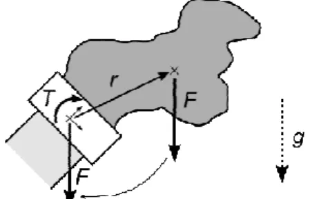
Fig. 3. Force and torque of a calibration body under gravitational pull

With a suitable pan/tilt unit or a robot, a variety of forces and torques can be applied to a sensor with only one well defined load just by positioning the load and the sensor in different angles to the gravitational pull (fig. 3).

The force torque sensors sees the force F and the torque T in its coordinate system. The force F itself is only the effect of the rigid body mass m under the gravitational pull (vector g in the base coordinate system) rotated by the alignment of the sensor coordinate system to the base coordinate system.

.

g

m

T

=

F

R,sensor

⋅

(8) The torque T is also easily defined by the cross product of F and the location of the centre of gravity of the calibration body:

.

F

r

=

T

×

(9) With the forces and torques combined to the measurement vector and the corresponding signal values, the acquisition of a lot of data points can be accomplished easily by just changing the alignment of the sensor and the calculation of the data with the alignment and calibration body information.

However there is a problem with 6DoF sensors, because there are dependencies between all forces and torques when using only one calibration body. These dependencies lead to a deficient rank in the load and signal matrices, which in turn can then not be inverted for the calculation of the calibration matrix.

The problem of the deficient rank can be solved by using more than one calibration body or one reconfigurable calibration body. In the example given in (fig. 4) it is possible to attach rods to different sides of the central cube of the calibration body. The geometrical design (cf.[1]) makes it easy to calculate the precise centre of gravity of the assembled body and on the other hand, the assembly of various configurations can carried out in very short time.

With the shown level of automation the calibration process can be much less time consuming, because the duration for measuring one data point is only the amount of time necessary for stopping the movement from one point to another. On the other hand a great amount of data can be acquired with very little interaction, which makes

(4)

a very precise calibration affordable. The mechanical actuation can be either carried out by a standard robot or pan tilt unit with appropriate angular measurement precision.

Yet there is still room for improvement, because the whole calibration procedure needs high precision orientation measurement in every step. Data acquisition during slow movement or without proper orientation measurement leads to low precision or faulty calibration results.

3. Shape from motion for calibration

The shape from motion approach summed up here has been described in [1] and subsequent articles, the notation used here goes along with the notation in this publication. The basic idea of the shape from motion approach for the calibration of force torque sensors is the observation, that too much high precision data is used during the LS procedure described above. It should be possible to extract information about the behaviour of the sensor just by looking at data gathered in a calibration measurement situation with some basic known facts, such as the mechanical properties of a calibration body.

3.1. Calibration algorithm

The calibration strategy starts again at (5) with the (n ×m) load matrix M, the (n ×p) signal matrix Z and the shape matrix S. The signal matrix is now analysed with singular value decomposition (SVD) [2]

,

T

V

Σ

U

=

Z

⋅

(10) which produces the orthogonal matrices: U(n × n), VT(p × p) and the zero-padded diagonal matrix ∑(n ×p) with the singular values in descending order on the diagonal.

With the rank rS of the measurement matrix this can be

rewritten to

,

T

V

Σ

U

=

Z

∗ ∗ ∗ ∗ (11) where U* consists of the first rS columns of U, ∑*is the

diagonal matrix of the rS first singular values and V*T

consists of the first rS rows of V T

. Because Z* is the best projection of Z into an rS-space, it is possible to combine

(5) and (11) into

,

S

M

=

V

Σ

U

=

Z

∗ ∗ ∗ ∗T (12)

from which estimates for M and S can be made (acc. [1]):

( )

T

V

Σ

=

S

Σ

U

=

M

∗ ∗ ∗ ∗ 2 / 1 ^ 2 / 1 ^ (13)

These estimates are not now the real motion (load) and shape matrices, but they are indeterminate by an indefinite transformation A:

.

^ 1 ^ ^ ^

























₋

S

A

M

=

S

M

(14)

So the task at hand is to find an invertible matrix A(r × r) which fulfils ^ 1 ^

S

A

=

S

A

M

=

M

− (15)

The first equation in (15) is not solved directly, but it can be solved by the knowledge about the measurement situation as mentioned at the beginning of this section. The resulting shape matrix is not now the real shape matrix, but it is arbitrarily scaled and rotated. Therefore a small number of measurements with known loads has to be introduced. From this loads a scaling and rotation matrix can be obtained, which can then be used for the computation of the shape matrix.

The rest of the calibration simply consists in inverting A and calculating the shape matrix S which can in turn be inverted and transposed to obtain the calibration matrix

( )

_T T

( )

₊ T T

S

=

SS

S

=

C



_



−1



_



(16)

The so introduced shape from motion approach for the calibration of force torque sensors further simplifies the process of the data acquisition under the cost of increasing the computational overhead.

As the data acquisition process has to be carried out for every single unit and this process is very time consuming, the cost of computational overhead is negligible. After the initial adjustment of the algorithm to a class of sensors and the calibration body (degrees of freedom and geometrical data) there are no changes or additional decisions needed. The algorithm can be just fed with any number of data points and reveals the calibration matrix without further interaction. On average personal computers the time needed for the calculations is in the range of a few seconds.

3.2. Calibration of a 6DoF sensor

The data acquisition for the calibration with the shape from motion algorithm uses a calibration body as described above for the automated data acquisition process. Hence the combined force torque vector of the loads becomes with (8, 9)

[

]

            − − − ⋅ 0 1 0 0 0 0 1 0 0 0 0 1 ~ x y x z y z T T T r r r r r r F = T F = m (17)

Unfortunately this means, that the resulting load matrix M from (5) will only have rank 3, where rank 6 would be

(5)

desirable to obtain the shape matrix. When using new notations (cf. [1]) for the final shape matrix

S

~

and the full load matrix

M

~

, which originates from (17), the following equation can be written down.

MS = S r r r r r r M = S M x y x z y z ~ 0 1 0 0 0 0 1 0 0 0 0 1 ~ ~             − − − (18)

From (18) it becomes clear, that the moment arm r becomes embedded into the shape matrix S, which can be computed by the shape from motion algorithm:

[ ]

IX

S

=

S

~

(19) To remove the moment arm r in order to find the desired final shape matrix it is necessary to carry out three data acquisition trials, because it is not possible to simply invert the matrix [I X]. Each of these trials is carried out constructing a different moment arm by reconfiguration of the calibration body.

The rank for one trial in (11) is rS = 3 and it is thereby

possible to compute

^

M

in (13). To now determine a correct transformation matrix A (15) it is necessary to apply knowledge about the forces in M. A single vector in M is in this special trial case is

[

x y z

]

T

i

=

f

m

(20) and this make it possible to see one simple constraint, which can be used for finding an appropriate transformation: the length of all these vectors is the same. This can also be brought further to the assumption, that the length is 1, because scaling and orienting the shapes has to be done in the following steps anyway. Therefore it is possible to state

1

1 ^ =! T i T i

=

m

A

m

⋅

− (21) which leads to a system of n equations that can be solved in 2 steps (the following lines use aij for the elements of A-1 and mij for the elements of

^

M

):

(

) (

)

(

)

(

)

(

)

1 2m 2m 2m 33 23 32 22 31 31 33 13 32 12 31 11 23 13 22 12 21 11 2 33 2 32 2 31 2 2 23 2 22 2 21 2 2 13 2 12 2 11 2 =! i3 i2 i3 i1 i2 i1 i3 i2 i1 a a + a a + a a m + a a + a a + a a m + a a + a a + a a m + a + a + a m + a + a + a m + a + a + a m (22) The first step is to solve for the 6 bracketed terms in the least squares sense [4]. In the second step a numerical solution is computed for those expressions [5]. The remaining degrees of freedom can be used to give the

matrix A a good shape (triangular or symmetrical). After finding the solution a solution for the shape matrix S is found by using (15). This shape is then scaled and oriented with some precise measurements with known loads and signals.

After evaluating all three trials and computing their shape matrices, the final shape matrix for all 6 dimensions has to be found. The solution for this problem can be found looking at (19) and the solutions of the 3 trials S1, S2 and

S3. By combining all moment arm embedding matrices

and shapes an equation for the extraction of the final shape matrix is revealed:

[ ]

IX

S

IX

=

S

~

3 2 1 3 2 1

⋅

























(23)

And (23) can be reformulated to

[ ]













⋅













3 2 1 3 2 1

~

S

IX

=

S

+ (24)

in order to get to the final shape matrix and thereby being able to compute the calibration matrix.

In summary the steps to adjust the calibration algorithm for a given type of 6 dimension force torque sensor consist of the selection of a proper calibration body, so that the combined matrix in (24) is invertible and choosing an a numerical solver for (22) in order to obtain the transformation matrix A. All other steps of the shape from motion algorithm remain the same as they are for every other sensor.

4. Implementation into a robot system

and evaluation of the calibration

Th calibration system for force torque sensors which has been constructed for the development of hardware and software structures has the following components: a KR-3 industry robot (KUKA Roboter GmbH), a sensor with 3 forces 3 torques – FDT mini45 (ATI Industrial Automation) connected to a PCI-ADC card and a standard PC with Matlab installed.

There are some special features in this system, which should be mentioned here: the robot is directly controlled by the PC using a real-time capable extension of Matlab

and the robot software component KUKA.

RobotSensorInterface which makes it possible to directly influence the robot controller. The second part is the modular software structure which is heavily based on a object oriented model of sensors and the various calibration algorithms. This structure makes it possible to exchange the various parts easily and it also allows the integration of other sensors with different interfaces or the evaluation of algorithms and computation modules.

(6)

The modular structure makes is also possible to scale the research platform down to a specific application.

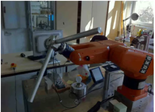
The following experiments have been carried out, using a reconfigurable aluminium calibration body with 2 detachable rods (fig. 4).

Fig. 4. Robot with mounted Calibration Body

The rods have been used to generate various locations of the centre of gravity. The mechanical properties of the calibration body are:

weight (g) dimensions (mm)

base 625 60x70x70

rod 411 300x25

As an example the 6 dimension force torque sensor has been calibrated with the calibration body. As a data base 170 measurements per trial have been made in equally spaced directions of the resulting force vector. Due to security concerns in the robot lab the speed of the robot was decreased, the measurements for one trial took about 5 minutes. Counting one additional trial for evaluation purposes and the time needed for mounting and reconfiguring the calibration body, the total time for the calibration is still below 30 minutes, which is an enormous speed up in comparison to the manual calibration procedure.

With a defined rated load of the sensor of ±15N in each force dimension and ±1Nm in the torque dimensions, the achievable precision measured during evaluation was better than 0.72% of the end value for the forces and below 0.3% for the torques. Unfortunately a false reading in the sensors z-Axis led to comparably high errors in this axis around 11%. These values are actually better than the values that can be obtained with the manufacturer supplied calibration values. However the direct comparison with those values suffers of the fact that the supplier calibration has been made for a much broader range of values and is thereby not this accurate for a small region of the sensor capacity.

Fig. 5. Recovered Force Vectors on a Sphere

In another experiment, the length of the applied force vector has been tested. As the load is not changed during one trial, all recovered force vectors should lie on a sphere (fig. 5). This test also showed very good results and was better than the results obtained manufacturers calibration matrix.

6. Conclusion and further work

In the works presented various approaches for the calibration of force torque sensors have been investigated and their features have been evaluated and discussed. The most promising approach to the solution of the calibration problem in robotic force and torque sensors is the shape from motion algorithm adapted form [1].

The future aim is further investigation in a method to calibrate force torque sensors during their use and without disassembling the application. Another very interesting topic is the transfer of the complete calibration procedure away from a personal computer directly into the sensor. So called intelligent sensors with completely integrated data processing capabilities are already available on the market. Unlike a system with an external interface to the robot these sensors cannot directly gather information on the actual position or orientation. Therefore it is necessary for an intelligent calibration to use as less as possible precise measurements as possible.

References

1. Richard M.Voyles, Jr., J. Daniel Morrow, Pradeep K. Khosla . “Shape from Motion Approach to Rapid and Precise Force/Torque Sensor Calibration”. In: Proc. of the ASME Dynamic Systems and Control Division, DSC-Vol. 57–1, San Francisco, CA, 1995.

2. Klema V. C., Laub A. J. “The Singular Value Decomposition: Its Computation and Some Applications”. In: IEEE Trans. on Automatic Control. 1980. Vol. 25, N 2. P. 164–176.

3. Forsythe G. E., Malcolm M., Moler C. B. “Computer Methods for Mathematical Computations”, Prentice Hall, Englewood Cliffs, NJ., 1977

4. D. Marquardt: An Algorithm for Least-Squares Estimation of Nonlinear Parameters, SIAM J. Appl. Math. 11, 431–441, 1963.

Techniques for Robotic Force Sensor Calibration