A Framework for Rendering Large Time-Varying Data Using Wavelet-Based
Time-Space Partitioning (WTSP) Tree
Chaoli Wang∗
Department of Computer and Information Science The Ohio State University
Han-Wei Shen†
Department of Computer and Information Science The Ohio State University
Abstract
We present a new framework for managing and rendering large scale time-varying data using the wavelet-based time-space parti-tioning (WTSP) tree. We utilize the hierarchical TSP tree data structure to capture both spatial and temporal locality and coher-ence of the underlying time-varying data and exploit the wavelet transform to convert the data into a multiresolution spatio-temporal representation. Coupled with the construction of TSP tree, a two-stage wavelet transform process (3D+1D) is applied to the data in the spatial and temporal domains respectively at the preprocess-ing step. Durpreprocess-ing renderpreprocess-ing, the wavelet-compressed data stream is decompressed on-the-fly and rendered using 3D hardware texture mapping. WTSP tree allows random access of data at arbitrary spa-tial and temporal resolutions at run time. The user is provided with flexible error control of image quality and rendering speed tradeoff. We demonstrate the effectiveness and utility of our framework by rendering gigabytes of time-varying data sets on a single off-the-shelf PC.
CR Categories: E.4 [Coding and Information Theory]: Data compaction and compression; I.3.3 [Computer Graphics]: Pic-ture and Image Generation—Viewing algorithms; I.3.6 [Computer Graphics]: Methodology and Techniques—Graphics data struc-tures and data types; I.3.6 [Computer Graphics]: Methodology and Techniques—Interaction techniques
Keywords: time-varying data, WTSP tree, wavelet transform, multiresolution, volume rendering
1
Introduction
While direct volume rendering with 3D hardware texture map-ping technique makes it possible to render three-dimensional time-invariant or time-varying data at interactive frame rates, the formidable challenge for interactive volume rendering is the huge amount of data. Nowadays, a typical time-varying data generated on rectilinear grids can have hundreds or thousands of time steps, and each time step may contain millions or billions of voxels. The sheer size of such time-varying volume data may range from giga-bytes to teragiga-bytes. Not surprisingly, data of this scale is overwhelm-ing the underlyoverwhelm-ing computational resources. Although a soverwhelm-ingle off-the-shelf PC or workstation today can be equipped with several gi-gabytes of main memory, and a consumer level graphics card now has several hundred megabytes of texture memory, transferring the data between disk and main memory, and between main memory and texture memory can become a bottleneck due to the limited bandwidth of memory systems. This constraint makes it very dif-ficult or virtually impossible to render a very large data set on a single PC or workstation without resorting to any compression or multiresolution scheme.
∗e-mail:[email protected]
†e-mail:[email protected]
To analyze complex dynamic phenomena from a large time-varying data set, it is necessary to navigate and browse the data in both the spatial and temporal domains, select data at different levels of detail, experiment with different visualization parameters, and compute and display selected features over a period of time. To achieve these goals, in this paper we present a new framework for managing and rendering large scale time-varying data. A data structure, called a wavelet-based time-space partitioning (WTSP)
tree, is designed for storing large scale time-varying data
hierar-chically. The input data is converted into a blockwise hierarchi-cal wavelet-compressed multiresolution representation in the pre-processing step. During rendering, the wavelet representation is decompressed on-the-fly and rendered using 3D hardware texture mapping. The WTSP tree data structure offers the following unique features. First, it exploits both spatial and temporal locality and coherence of the underlying time-varying data, thus allowing ran-dom access of data at arbitrary spatial and temporal resolutions at run time. Second, by utilizing wavelet transform and compression, lossy or lossless compression could be achieved with reasonable compression rate and affordable cost for data compression and de-compression. Third, the user is provided with flexible error control for image quality and rendering speed tradeoff at run time. Finally, the blockwise data partition scheme and hierarchical WTSP tree structure make our framework suitable for large-scale out-of-core application and parallel rendering scheme.
The remainder of the paper is structured as follows. We first review related work in Section 2. In Section 3, we describe how to construct the wavelet-based data hierarchy for large scale time-varying data using the WTSP tree and how to calculate spatial and temporal errors. Section 4 discusses WTSP tree traversal, data re-construction, rendering acceleration and caching strategy. Results are given in Section 5 and the paper is concluded in Section 6 with the future directions for our research.
2
Related Work
Previous work on time-invariant or time-varying data visualization that relates to our work primarily focused on designing hierarchical multiresolution data representation techniques as well as effective wavelet transform and compression schemes.
Having the ability to visualize data at different resolutions allows the user to identify features in different scales, and to balance image quality and computation speed. Along this direction, a number of techniques have been introduced to provide hierarchical data rep-resentation for volume data. Burt and Adelson [Burt and Adelson 1983] proposed the Laplacian Pyramid as a compact hierarchical image code. This technique was extended to 3D by Ghavamnia and Yang [Ghavamnia and Yang 1995] and applied to volumetric data. Their Laplacian pyramid is constructed using a Gaussian low-pass filter and encoded by uniform quantization. Voxel values are recon-structed at run time by traversing the pyramid from bottom to top. To reduce the huge reconstruction overhead, they suggested a cache data structure. LaMar et al. [LaMar et al. 1999] proposed an
octree-based hierarchy for volume rendering where the octree nodes store volume blocks resampled to a fixed resolution and rendered using 3D texture hardware. A similar technique was introduced by Boada
et al. [Boada et al. 2001]. Their hierarchical texture memory
rep-resentation and management policy benefits nearly homogeneous regions and regions of lower interest.
For time-varying data hierarchical representation, Finkelstein
et al. [Finkelstein et al. 1996] proposed multiresolution video, a
representation for time-varying image data that allows for varying spatial and temporal resolutions adaptive to the video sequence. An approach dealing with large-scale time-varying fields was described by Shen et al. [Shen et al. 1999]. The data structure, called the
time-space partitioning (TSP) tree, captures both the spatial and
tempo-ral coherence of the underlying data. Ellsworth et al. [Ellsworth et al. 2000] later followed up the work in [Shen et al. 1999] and provided a hardware volume rendering algorithm using a TSP tree and proposed color-based error metrics that improve the selection of texture volumes to be loaded into texture memory. Linsen et al. [Linsen et al. 2002] presented a four-dimensional multiresolution approach for time-varying volume data that supports a hierarchy with spatial and temporal scalability. In their scheme, temporal and spatial dimensions are treated equally in a single hierarchical framework.
Wavelets are a mathematical tool for representing functions hi-erarchically, and have gained much popularity in several areas of computer graphics [Stollnitz et al. 1996] due to their favorable properties such as vanish moments, hierarchical and multiresolu-tion decomposimultiresolu-tion structure, linear time and space complexity of the transformation, decorrelated coefficients, and a wide variety of basis functions [Li et al. 2002]. Over the past decade, many wavelet transform and compression schemes have been applied to volumet-ric data. Muraki [Muraki 1992; Muraki 1993] introduced the idea of using the wavelet transform to obtain a unique shape descrip-tion of an object, where 2D wavelet transform is extended to 3D and applied to eliminate wavelet coefficients of lower importance. Using single 3D [Ihm and Park 1998; Kim and Shin 1999] or mul-tiple 2D [Rodler 1999] Haar wavelet transformations for large 3D volume data has been well studied, resulting in high compression ratios with fast random access of data at run time. More recently, Guthe et al. [Guthe et al. 2002] presented a hierarchical wavelet representation for large volume data sets that supports interactive walkthroughs on a single commodity PC. Only the levels of detail necessary for display are extracted and sent to texture hardware for the current viewing.
For time-varying data compression schemes, Ma and Shen [Ma and Shen 2000] used octree encoding and difference encoding for spatial and temporal domain compression respectively. They also investigated how quantization might affect further compres-sion, rendering optimization and image results of time-varying data. Lum et al. [Lum et al. 2002] proposed to use DCT to encode indi-vidual voxels along the time dimension, and employed a color table animation technique to render the volumes using texture hardware. Guthe and Straßer [Guthe and StraBer 2001] introduced an algo-rithm that uses the wavelet transform to encode each spatial vol-ume, and then applies a windowed motion compensation strategy to match the volume blocks in adjacent time steps. Sohn et al. [Sohn et al. 2002] described a compression scheme where wavelet trans-form is used to create intra-coded volumes and difference encoding is applied to compress the time sequence. While all these methods can perform efficient data compression and rendering, their goals are not for supporting flexible spatio-temporal multiresolution data browsing. Some of these methods also require pre-defined quality thresholds to perform encoding, and thus are lossy by nature.
3
Wavelet-Based Time-Space Partitioning
(WTSP) Tree
Although data encoding for spatial volumes and videos has been studied intensively, transformation and management of large scale three-dimensional time-varying data still require further investiga-tion. In this paper, we propose an effective data encoding and management scheme to facilitate interactive browsing of spatio-temporal multiresolution data. The primary goals of our work is to decorrelate the time-varying data into a range of spatial and tem-poral levels of detail, and to develop efficient data management scheme to enable rapid run-time data retrieval and reconstruction. To achieve these goals, in the following we describe a wavelet-based data encoding scheme with minimal space overhead and an efficient data structure used to organize the encoded data.
3.1 Wavelet Transform and TSP Tree
A wavelet transform projects the input signal into an orthogonal or biorthogonal basis space spanned by functions called wavelets. Wavelets can be used to transform a data set into a multiresolution representation consisting of a collection of coefficients, where each coefficient corresponds to a particular frequency and spatial compo-nent decomposed from the original data. The efficiency of wavelets in data compression stems from their unique ability in approximat-ing non-linear and non-stationary signals with only a few non-zero coefficients, which leads to a compact representation of the original function. Previously, researchers have shown that wavelet-based compression can provide good visual quality with a high compres-sion rate [Khali et al. 1999].
To apply the wavelet transform to 3D time-varying volume data, a straightforward approach is to perform a 4D wavelet transform, where time is treated as the fourth dimension. To create a mul-tiresolution data hierarchy, one can extend the algorithm proposed by Guthe et al. [Guthe et al. 2002] for static volumes to four di-mensions, where the space-time wavelet coefficients are stored in a 4D tree, or called 16-tree. A 16-tree treats time merely as another dimension. Using a method similar to the spatial subdivision for octree construction, each node in the 16-tree has sixteen children instead of eight. Although simple to implement, the 16-tree can be ineffective for two reasons. First, there could be large discrep-ancy between the spatial and temporal dimensions, which makes it difficult to subdivide the spatial and temporal dimensions uni-formly. Furthermore, in 16-trees, the temporal and spatial domains are tightly coupled in the hierarchical subdivision, which means it could be difficult to choose an arbitrary combination of spatial and temporal data resolutions from the 4D hierarchy.
To remove the dependency between spatial and temporal res-olutions, we propose a wavelet-based time-space partitioning (WTSP) tree to store the wavelet transformed time-varying three-dimensional data. The TSP tree [Shen et al. 1999] is a time-supplemented octree. In essence, the skeleton of a TSP tree is a standard complete octree, which recursively subdivides the volume spatially until all subvolumes reach a predefined minimum size. In each of the TSP tree nodes (we call it spatial node hereafter), a bi-nary time tree is created, where each node in the bibi-nary time tree (we call it temporal node hereafter) represents a spatial subvolume with a different time span. The unique advantage of TSP tree is that it allows the user to request spatial and temporal data resolutions independently with separate error thresholds. In this way, a flexible browsing of data at arbitrary spatio-temporal resolutions becomes possible. In the following, we describe the construction of WTSP tree in detail.
3.2 WTSP Tree Construction
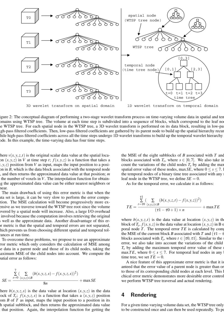
The WTSP tree is a space-time hierarchical data structure used to organize the spatio-temporal wavelet coefficients. The design goal of the WTSP tree is to support interactive browsing of data at ar-bitrary spatio-temporal scales. To construct the WTSP tree, a two-stage wavelet transform process is performed. First, we subdivide the volume at each time step into a sequence of blocks. A method similar to [Guthe et al. 2002] is used to perform a 3D wavelet trans-form for each of the spatial blocks. This will produce a volume hi-erarchy in the form of a complete octree for every time step, where each spatial node represents a subvolume with a different resolution in space. For the spatial nodes that correspond to the same spatial region and resolution in a sequence of time steps, we perform a 1D wavelet transform to build a temporal hierarchy for each subvol-ume. Using Haar wavelets, we can build a binary time tree asso-ciated with each of the spatial nodes with a method similar to the
error tree algorithm [Matias et al. 1998] (shown in Figure 1). This
1D wavelet transform process merges all the spatial octrees across time to build a single spatio-temporal hierarchical data structure. The temporal hierarchy stores the multiresolution temporal wavelet hierarchy at the corresponding spatial region and resolution. A con-ceptual diagram of our algorithm is shown in Figure 2.
A[0,3] & D[0,3]
D[0,1] D[2,3]
V0
V1 V2 V3
A[0,1] A[2,3]
Figure 1: Building the temporal hierarchy on a time tree associated with each of the spatial nodes using 1D wavelet transforms. Using Haar wavelets, we can build the binary time tree from bottom to up in an error tree style. A[τ0,τ1] represents the average value across time span [τ0,τ1], D[τ0,τ1] stands for difference value across time span [τ0,τ1], and Vt is the data value at time step t. In this example, the time-varying data has four time steps. During the preprocessing, we compute and store A[0,3] and D[0,3] at the temporal root node, and D[0,1] and D[2,3] in its left and right child nodes respectively. At run time, these four values are used to reconstruct average values A[0,1], A[2,3] and value Vt at time step t by traversing the time tree from top to down.
The construction of the WTSP tree for the input time-varying volume data set is performed in the preprocessing step. We take a blockwise wavelet transform and compression strategy to achieve efficient data decompression and support random access of data at run time. Assuming that the block size, n is nx×ny×nz, where nx=2i, ny=2jand nz=2kwith i, j and k all integers and greater than 1, we now describe the bottom-up algorithm for building the WTSP tree.
For each of the raw volume block, a 3D wavelet transform is first performed. This will produce low-pass filtered coefficients of size n/8 and high-pass filtered coefficients of size 7n/8. The low-pass filtered wavelet coefficients from eight adjacent subvolumes are collected and grouped into a single block of n voxels, which will become the parent node of the eight subvolumes in the spa-tial octree hierarchy. We recursively apply this 3D wavelet trans-form and coefficient grouping process until the root of the octree is reached. As we arrive at the WTSP tree root node, since the root
node has no parent node, no recursive 3D wavelet transforms will be performed. To reduce the size of the coefficients stored in the octree, the high-pass filtered coefficients resulting from the wavelet transform will be compared against a user-provided threshold. The high-pass filtered coefficients are set to zero if they are smaller than the threshold.
The above 3D wavelet transform is performed for the data at every time step. To create a temporal hierarchy, we apply 1D wavelet transforms to the high-pass filtered coefficients from the corresponding spatial node along the time axis. The high-pass fil-tered coefficients resulting from the 1D wavelet transform is then compressed using run-length encoding combined with a fixed Huff-man encoder [Guthe et al. 2002]. The compressed bit streams are saved into separate files. Finally, we build a binary time tree associ-ated with each spatial node, and then compute spatial and temporal errors for each of the temporal nodes in the time tree.
To save space and time during the WTSP tree construction pro-cess, several checks can be done in advance to avoid unnecessary wavelet transform computation. First, if the data block is uniform, we can skip the 3D wavelet transform process and set the low-pass filtered coefficients to the uniform value and the high-pass filtered coefficients to zero. Second, if the high-pass filtered coefficients of the corresponding spatial nodes in the time sequence are all zeros, we can skip the 1D wavelet transform process all together.
As each spatial node can be identified by a spatial id, sid, and each temporal node in a time tree can have a specific temporal id,
tid, the wavelet coefficients stored in any temporal node can be
uniquely identified by a name composed of its corresponding sid and tid. In our implementation, we store the coefficients associ-ated with a spatial node into a list of files. Because the number of such coefficient files may be easily over thousands for large time-varying data, coefficient files are organized into different directories depending on the corresponding sid for easy access.
3.3 Error Metrics
When constructing the WTSP tree, spatial and temporal errors are calculated for every temporal node in each of the binary time trees. We present two types of error metrics, which are both based on mean square error (MSE) calculation. The first one is based on the MSE between the lower spatial and temporal resolution data block and the original data. This metric is slow to compute when the underlying time-varying data set is large. As an alternative, we can use an approximate metric, which represents the MSE among the data in a “parent” node and its “child” nodes, taking the maximum MSE of the child nodes into account. This metric is in general faster to compute. We follow the denotations defined below when we discuss the formulae used to calculate the error metrics:
For a data block B of n voxels associated with the current tem-poral node T at a specific spatial (representing the original spatial subvolume V ) and temporal (across time steps fromτ0 toτ1) res-olutions, let S be its corresponding spatial node. Let the sth spatial child node of S be Ss, and the corresponding temporal node of Ss with the same tid as T be Ts, where s∈[0,7]. Let the tth temporal leaf node of T in the time tree be Tt, where t∈[τ0,τ1]. For the convenience of discussion, in this paper we treat the relationship between T and Tsas a “parent-child” relationship.
The first error metric calculates the MSE between the low reso-lution data block B and the corresponding raw volume data V across time steps fromτ0 toτ1. To calculate the error, we use the follow-ing formula: ST E= τ1 ∑ t=τ0 ( ∑ (x,y,z)∈V (v(x,y,z,t)−f(x,y,z))2) (τ1−τ0+1)×m
T0 T1 T2 T3 [0,3] [0,1] [2,3] t=0 t=1t=2 t=3
3D wavelet transform on spatial domain 1D wavelet transform on temporal domain
WTSP tree
time tree spatial node
(WTSP tree node)
temporal node (time tree node)
Figure 2: The conceptual diagram of performing a two-stage wavelet transform process on time-varying volume data in spatial and temporal domains using WTSP tree. The volume at each time step is subdivided into a sequence of blocks, which correspond to the leaf nodes of the WTSP tree. For each spatial node in the WTSP tree, a 3D wavelet transform is performed on its data block, resulting in low-pass and high-pass filtered coefficients. Then, low-pass filtered coefficients are gathered by its parent node to build up the spatial hierarchy recursively while high-pass filtered coefficients across all the time steps undergo 1D wavelet transforms to build up the temporal wavelet hierarchy at that node. In this example, the time-varying data has four time steps.
where v(x,y,z,t)is the original scalar data value at the spatial loca-tion(x,y,z)in V at time step t; f(x,y,z)is a function that takes a (x,y,z)position from V as input, maps the input position to a posi-tion in B, which is the data block associated with the temporal node
T , and then returns the approximated data value at that position; m
is the number of voxels in V . The interpolation function for obtain-ing the approximated data value can be either nearest neighbors or linear.
The main drawback of using this error metric is that when the data set is large, it can be very slow to perform the error compu-tation. The MSE calculation will become progressively more ex-pensive as we traverse toward the WTSP tree root since the volume covered by a spatial node will increase. Also, a large I/O overhead is involved because the computation involves retrieving the original as well as the approximate data. Another disadvantage of this er-ror metric is that the spatial and temporal erer-rors are not separated, which prevents us from choosing different spatial and temporal tol-erances at run time.
To overcome these problems, we propose to use an approximate error metric which only considers the calculation of MSE among the data in a parent node and those of its child nodes, taking the maximum MSE of the child nodes into account. We compute the spatial error as follows:
SE= 7 ∑ s=0 ( ∑ (x,y,z)∈B (b(x,y,z,s)−f(x,y,z,s))2) 8n +max SE
where b(x,y,z,s) is the data value at location(x,y,z)in the data block of Ts; f(x,y,z,s)is a function that takes a(x,y,z) position from B of T as input, maps the input position to a position in its
sth spatial subblock, and then returns the approximated data value
at that position. Again, the interpolation function for getting the approximated data value could be either nearest neighbors or lin-ear. Essentially, the spatial error SE is calculated by computing
the MSE of the eight subblocks of B associated with T and eight blocks associated with Ts, where s∈[0,7]. We also take into ac-count the variations of the child nodes Tsby adding the maximum spatial error value of these nodes, max SE, where 0≤s≤7. For all the temporal nodes of a binary time tree associated with any spatial leaf node in the WTSP tree, we define SE=0.
As for the temporal error, we calculate it as follows:
T E= τ1 ∑ t=τ0 ( ∑ (x,y,z)∈B (b(x,y,z,t)−f(x,y,z))2) (τ1−τ0+1)×n +max T E
where b(x,y,z,t) is the data value at location(x,y,z)in the data block of Tt, f(x,y,z)is the data value at location(x,y,z)in B of tem-poral node T . The temtem-poral error T E is calculated by computing the MSE of the current block B associated with T and(τ1−τ0+1) blocks associated with Tt, where t∈[τ0,τ1]. Similar to the spatial error, we also take into account the variations of the child nodes
Ts by adding the maximum temporal error value of these nodes, max T E, where 0≤s≤7. For temporal leaf nodes in any binary time tree, we set T E=0.
A nice feature of this approximate error metric is that it is guar-anteed that the error value of a parent node is greater than or equal to those of its corresponding child nodes at each level. This hierar-chical error metric demonstrates more desirable error control when we perform WTSP tree traversal and actual rendering.
4
Rendering
For a given time-varying volume data set, the WTSP tree only needs to be constructed once and can then be used repeatedly. To perform volume rendering, the WTSP tree is first traversed to identify the subvolumes that satisfy the user-specified error tolerances. These
subvolumes are then reconstructed from their wavelet representa-tions and rendered in the correct depth order to generate the final image. In this section, we first briefly describe WTSP tree traver-sal and data block rendering, then discuss acceleration and data caching strategies to facilitate run-time volume rendering. 4.1 WTSP Tree Traversal and Rendering
The WTSP tree traversal is similar to the traversal algorithm pre-sented in [Shen et al. 1999]. We traverse both the WTSP tree’s octree skeleton and the binary time tree associated with each en-countered spatial node. At run time, the user specifies the time step and the tolerances for both spatial and temporal errors. The nodes in the WTSP tree are recursively visited in the front-to-back visibil-ity order according to the viewing direction. The tolerance for the spatial error provides a stopping criterion for the octree traversal so that the regions having tolerable spatial variations can be rendered using lower spatial resolutions. The tolerance for the temporal er-ror is used to identify regions where it is appropriate to use data of lower temporal resolutions due to their small temporal variations. This allows us to reuse the data of those subvolumes for multiple time steps. The result of the tree traversal is a series of subvolumes with different size and characteristics of spatial and temporal co-herence. The corresponding data blocks in the subvolumes from the traversal are reconstructed and then rendered using 3D texture hardware. The final image is constructed by compositing colors and opacities of the partial images. For a more detailed description of the traversal algorithm, please refer to [Shen et al. 1999].
4.2 Data Block Reconstruction
If a subvolume at a certain spatial and temporal resolution satisfies the user-specified error tolerances during tree traversal, and the as-sociated data block has not been reconstructed and cached in main memory previously, we need to reconstruct the data block before the rendering is performed.
If the spatial node corresponding to the current temporal node is the WTSP tree root node, we retrieve the data block of n voxels from its time tree hierarchy according to the time step in question. The corresponding wavelet transformed block files are accessed, and inverse 1D wavelet transforms are performed to reconstruct the data block.
If the corresponding spatial node is a WTSP tree non-root node, we recursively request the data block associated with its parent node, and reconstruct the corresponding data blocks if necessary. This is to collect the low-pass filtered coefficients of size n/8 from the data block associated with its parent node. The correspond-ing high-pass filtered coefficients of size 7n/8 are obtained from its time tree hierarchy by decoding corresponding bit file streams and applying inverse 1D wavelet transforms. Finally, we group the low and high pass filtered coefficients into a single block of n voxels and apply an inverse 3D wavelet transform to reconstruct the data block.
4.3 Acceleration Techniques and Caching Strategy During run-time rendering, several acceleration techniques can be utilized to reduce the data reconstruction overhead and improve the rendering speed:
• Identify and cull away blocks outside of the current
view-ing frustum to minimize the computation and I/O overhead. These invisible blocks will not have any contribution to the final image so no wavelet reconstruction should be performed on them.
• Given a new viewing direction, refrain from reconstructing
blocks with screen projection size less than a predefined small threshold value while reconstructing and rendering other visi-ble blocks in the first few frames, because they will contribute little to final image generated. These blocks with small pro-jection size could be reconstructed and added into the render-ing pipeline progressively in follow-up renderrender-ing frames as a refinement, with the block ordering remaining the same as obtained from tree traversal.
• Skip empty blocks and render uniform blocks of non-zero data
values as polygons with pre-lookup colors and opacities, ob-viating texture loading and mapping.
Experiments showed that for blocks that are larger than 643, the time spent on reconstruction, i.e., applying the inverse 3D wavelet transform, could be longer than the time for data disk I/O and hard-ware texture mapping. Thus, appropriate caching of previously re-constructed data is critical for achieving better performance when visualizing large time-varying data sets. In addition, as we may anticipate reusing most of the reconstructed data blocks for subse-quent frames due to the spatial and temporal coherence exploited by the WTSP tree structure, it is desirable to cache the data blocks that have already been reconstructed.
To realize this idea, we propose a three-level hierarchical caching strategy using a least often used (LOU) block schedul-ing scheme combined with a prioritization of all the temporal nodes in the WTSP tree. The three level caches are disk, main memory and texture memory. Users define a fixed amount of disk space and main memory dedicated for the caching purpose. Upon requesting a data block for rendering, we use OpenGL
glAreTexturesResident()command to query the residency of
a subvolume’s texture. If the data block does not reside in texture memory, we useglBindTexture()to load the block from main memory to texture memory, provided the block is already cached in main memory. Otherwise, we need to load the data from the disk file, or reconstruct and then load it into main memory, depending on whether the reconstructed data block is cached on disk or not.
Every temporal node in the binary time tree associated with each of the spatial nodes keeps a counter recording how many times the data block at this node has been visited, taking the priority value of the node into account. A priority value is a positive integer asso-ciated with every temporal node, indicating which levels of WTSP tree and its corresponding time tree the node lies on. Since nodes closer to the WTSP tree spatial root node and its corresponding time tree temporal root node have higher chances to be requested than those nodes farther away from the root nodes, higher priority values are assigned to these temporal nodes. Whenever there is a main memory hit for a data block, the counter of the correspond-ing node increases by its priority value. At the time we run short of the available main memory for caching the intermediate results, our LOU replacement scheme will swap out a data block with smallest counter value.
5
Results
In this section, we discuss the experimental results obtained with an implementation of our algorithm. The algorithm was implemented in C++ and OpenGL, with nVidia extensions to perform volume rendering using 3D hardware texture mapping. All benchmarks were performed on a 2.0GHz Pentium 4 processor with 768MB main memory, and a nVidia GeForce FX 5600 graphics card with 128MB video memory.
data orig. comp. comp. total set size size ratio files BOB1 7.5GB 1.34GB 5.60:1 8,410 BOB4 30GB 1.52GB 19.74:1 21,667 BOB8 60GB 9.58GB 6.26:1 59,559
Table 1: Compression of three BOB data sets with lossless scheme. We achieved more than 5:1 compression ratios for all three data sets.
5.1 Data Set
The time-varying data used in our testing is a brick-of-byte (BOB) data set from Lawrence Livermore National Laboratory. The BOB data set [Mirin et al. 1999] was generated from a three-dimensional time-varying simulation of the Richtmyer-Meshkov instability and turbulent mixing in a shock tube experiment conducted at Caltech. The simulation result is stored in 274 time steps, and each time step has an associated 2048×2048×1920 rectilinear grids. For each grid point, an entropy value between 0 and 255 is stored. At each time step, the data is decomposed into 8×8×15 bricks and stored in 960 separated files, hence the name BOB. Overall, the size of each time step is 7.5GB and the total size of the whole data is over 2TB, stored in 263,040 different files.
Due to the space limit of our PC, we could use only a subset of the BOB data set to perform the tests. Three subsets of the BOB data, BOB1 (the 256th time step), BOB4 (starting from the 16th and picking every 16th time step, total 4 time steps), and BOB8 (starting from the 32th and picking every 32th time step, total 8 time steps) have been used in our experiment.
5.2 Preprocessing Result
In all cases, we chose the block size to be 128×128×64 and each block is of size 1MB. This is a tradeoff between the time to per-form the wavelet transper-form for a single data block and the render-ing overhead for final image generation. Since each voxel value is represented using a single byte, Haar wavelet transform with lift-ing scheme is adopted for both spatial 3D and temporal 1D wavelet transforms for simplicity and efficiency reasons. Lossless compres-sion scheme was used with the threshold set to zero and the approx-imate error metric was calculated for every temporal node in each of the binary time trees. We considered one voxel overlapping bound-aries between neighboring blocks in each dimension when loading data from original brick data files in order to produce correct ren-dering result. The WTSP tree was built by applying the two-stage wavelet transform process described in Section 3, and the error met-ric was computed in a bottom-up fashion during preprocessing. For all the three data sets, the constructed WTSP trees have a depth of six with 10,499 non-empty spatial nodes.
WTSP tree compression result of the three data sets is displayed in Table 1. We achieved more than 5:1 compression ratios in all three cases. The compression ratio for BOB4 is much higher than BOB1 and BOB8, this is because at early time steps, the BOB data has much less variation than later ones, thus providing more room for compression.
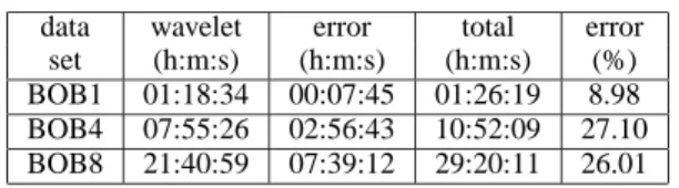
Table 2 shows the total time to construct the WTSP trees, which includes the time to perform wavelet transforms and to compute spatial and temporal errors. The percentage of time spent on error metric computation for BOB1 is much less than BOB4 and BOB8. This is because BOB1 only contains a single time step, and hence only spatial errors are calculated while temporal errors are zero for all the temporal nodes. Note that approximate error metric was used to generate the timing in the table, which accounts for at most 27.10% of the total time for all three BOB data sets. When we used
data wavelet error total error set (h:m:s) (h:m:s) (h:m:s) (%) BOB1 01:18:34 00:07:45 01:26:19 8.98 BOB4 07:55:26 02:56:43 10:52:09 27.10 BOB8 21:40:59 07:39:12 29:20:11 26.01
Table 2: WTSP tree construction time for three BOB data sets. The construction time includes time to perform wavelet transforms and time to calculate error metric, which only accounts for at most 27.10% of the total time for all three cases.
the other error metric discussed in Section 3.3 on BOB8, approx-imately, 80% of WTSP tree construction time was spent on error calculation, and the total time to construct the WTSP tree for BOB8 was about four days, compared to less than 30 hours as shown in the table when approximate error metric was used. Approximate error metric is much more efficient to compute than the other one, and was equally effective from our experimental studies.
5.3 Rendering Result
In all the test cases, we allocated 512MB main memory and 1GB disk space for caching. The resolution of the output image was 500×500 for all the tests. The opacity transfer function design is based upon the histogram of data values while the color changes from blue to magenta to cyan to green to yellow, as we increase the entropy value from 0 to 255. During rendering, a sequence of data blocks were identified in the visibility order, reconstructed and loaded if necessary, and then rendered using 3D texture hardware.
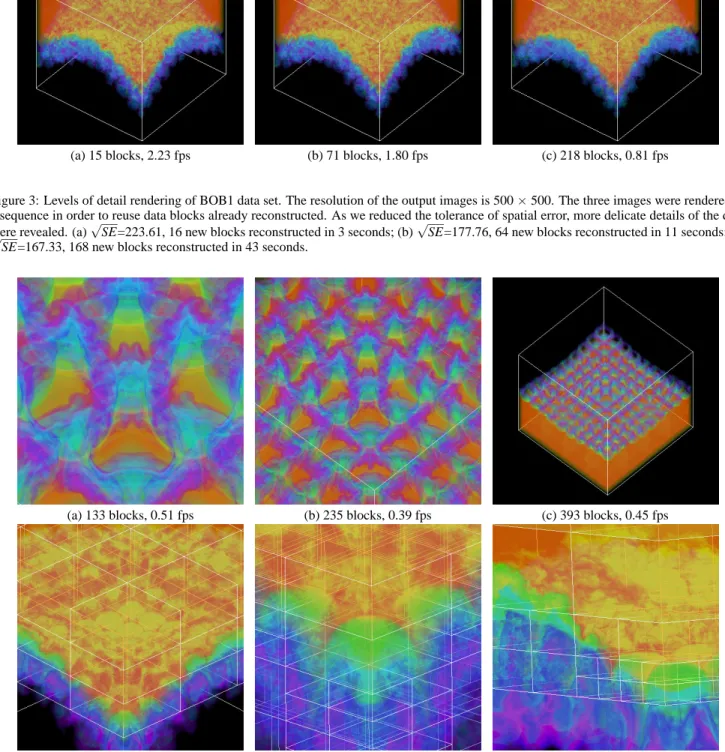
Figure 3 shows the rendering results of various levels of detail for the BOB1 data set. When the error tolerance became higher, data of lower resolutions were used, which resulted in a smaller number of blocks being rendered. It can be observed that although more delicate details of the data are revealed when reducing the spatial error tolerance, images of reasonable quality can still be obtained at lower resolutions. The use of wavelet-based compression also allowed us to produce rendering of good visual quality with much smaller space overhead. The reconstruction time listed in the fig-ure includes disk I/O to fetch low and high pass filtered coefficients of blocks, decoding the compressed bit streams, and performing the inverse wavelet transforms. Among those operations, our tests showed that most of the reconstruction time was spent on 3D in-verse wavelet transforms.
For time-varying data sets, BOB4 and BOB8, we performed ren-dering with different spatial and temporal error controls in order to test the flexibility and effectiveness of our algorithm. Figure 4 (a)-(c) show the rendering images when zooming out the BOB4 data set. As we zoomed out, more and more data blocks were identified and rendered. Utilizing caching scheme to capture spatial locality and coherence, data blocks reconstructed and cached in previous frames can be reused in the current frame. Thus, we can achieve relatively smooth transition among frames. (d)-(e) give three snap-shots of rendering BOB8 data with different spatial and temporal error tolerance values. We randomly picked three time steps and rendered them in an arbitrary order. Both spatial and temporal co-herences captured by WTSP tree structure were well exploited in the rendering and our caching scheme played an essential role in maintaining reasonable frame rates during the rendering process.
6
Conclusion and Future Work
We have presented a new framework for managing and rendering large time-varying data using the wavelet-based time-space parti-tioning (WTSP) tree. We utilize a hierarchical TSP tree data
struc-ture to capstruc-ture both spatial and temporal locality and coherence of the underlying time-varying data and exploit the wavelet transform to encode the data into a multiresolution spatio-temporal represen-tation. A two-stage wavelet transform process(3D+1D)is per-formed on the data in spatial and temporal domains respectively at the preprocessing step. During rendering, the wavelet-compressed data stream is decompressed on-the-fly and rendered using 3D hard-ware texture mapping. From the test results of running gigabytes time-varying data sets on a single PC, we demonstrate the capa-bility of random access of data at run time using WTSP tree and the flexibility of controlling the image quality and rendering speed tradeoff.
Future work includes studying different approaches to combine the WTSP tree data structure with other data compression schemes. For instance, we can incorporate the Laplacian pyramid structure into the WTSP tree and trade space for reconstruction and render-ing time. We will investigate the pros and cons of this option. As indicated in Section 5, the time to reconstruct data blocks using 3D inverse wavelet transforms dominates the rendering time. We will look into the solution of performing 3D wavelet transforms on graphics hardware in order to alleviate or eliminate this render-ing bottleneck. Previous work by Hopf and Ertl [Hopf and Ertl 1999] and the emergence of a hardware-oriented, general-purpose language - Cg [Mark et al. 2003] have shown the potential of ac-complishing this task in hardware. Since the size of WTSP tree rep-resentation for a large time-varying data set may still be too large to handle on a single PC or workstation, we will develop out-of-core time-critical rendering algorithm for dynamic levels of detail selec-tions. Finally, we would like to explore the idea of subdividing the WTSP tree into different branches, and distributing the multireso-lution data into a parallel or multi-server network visualization en-vironment for load balancing and network quality of service (QoS) adaptation.
References
BOADA, I., NAVAZO, I.,ANDSCOPIGNO, R. 2001. Multiresolution Vol-ume Visualization with a Texture-Based Octree. The Visual Computer 17, 3, 185–197.
BURT, P. J., ANDADELSON, E. H. 1983. The Laplacian Pyramid as a Compact Image Code. IEEE Transactions on Communications 31, 4, 532–540.
ELLSWORTH, D., CHIANG, L. J.,ANDSHEN, H. W. 2000. Accelerating Time-Varying Hardware Volume Rendering Using TSP Trees and Color-Based Error Metrics. In Proceedings of IEEE Symposium on Volume Visualization ’00, ACM Press, 119–129.
FINKELSTEIN, A., JACOBS, C. E.,ANDSALESIN, D. H. 1996. Multires-olution Video. In Proceedings of ACM SIGGRAPH ’96, ACM Press, 281–290.
GHAVAMNIA, M. H.,ANDYANG, X. D. 1995. Direct Rendering of Lapla-cian Pyramid Compressed Volume Data. In Proceedings of IEEE Visu-alization ’95, IEEE Computer Society Press, 192–199.
GUTHE, S., ANDSTRABER, W. 2001. Real-Time Decompression and Visualization of Animated Volume Data. In Proceedings of IEEE Visu-alization ’01, IEEE Computer Society Press, 349–356.
GUTHE, S., WAND, M., GONSER, J.,ANDSTRABER, W. 2002. Inter-active Rendering of Large Volume Data Sets. In Proceedings of IEEE Visualization ’02, IEEE Computer Society Press, 53–60.
HOPF, M.,ANDERTL, T. 1999. Accelerating 3D Convolution using Graph-ics Hardware. In Proceedings of IEEE Visualization ’99, IEEE Computer Society Press, 471–474.
IHM, I.,ANDPARK, S. 1998. Wavelet-Based 3D Compression Scheme for Very Large Volume Data. In Graphics Interface ’98, 107–116.
KHALI, H., ATIYA, A. F.,ANDSHAHEEN, S. 1999. Three-Dimensional Video Compression Using Subband/Wavelet Transform with Lower Buffering Requirements. IEEE Transactions on Image Processing 8, 6, 762–773.
KIM, T. Y.,ANDSHIN, Y. G. 1999. An Efficient Wavelet-Based Compres-sion Method for Volume Rendering. In Proceedings of Pacific Graphics ’99, IEEE Computer Society, 147–157.
LAMAR, E., HAMANN, B.,ANDJOY, K. I. 1999. Multiresolution Tech-niques for Interactive Texture-Based Volume Visualization. In Proceed-ings of IEEE Visualization ’99, IEEE Computer Society Press, 355–362. LI, T., LI, Q., ZHU, S.,ANDOGIHARA, M. 2002. A Survey on Wavelet Applications in Data Mining. ACM SIGKDD Explorations Newsletter 4, 2, 49–68.
LINSEN, L., PASCUCCI, V., DUCHAINEAU, M. A., HAMANN, B.,AND JOY, K. I. 2002. Hierarchical Representation of Time-Varying Volume Data with√42 Subdivision and Quadrilinear B-Spline Wavelets. In Pro-ceedings of Pacific Graphics ’02, IEEE Computer Society Press, 346– 355.
LUM, E. B., MA, K. L.,ANDCLYNE, J. 2002. A Hardware-Assisted Scal-able Solution for Interactive Volume Rendering of Time-Varying Data. IEEE Transactions on Visualization and Computer Graphics 8, 3, 286– 301.
MA, K. L.,ANDSHEN, H. W. 2000. Compression and Accelerated Ren-dering of Time-Varying Data. In Proceedings of the Workshop on Com-puter Graphics and Virtual Reality ’00.
MARK, W. R., GLANVILLE, R. S., AKELEY, K.,ANDKILGARD, M. J. 2003. Cg: A System for Programming Graphics Hardware in a C-like Language. In Proceedings of ACM SIGGRAPH ’03, ACM Press, 896– 907.
MATIAS, Y., VITTER, J. S.,ANDWANG, M. 1998. Wavelet-Based His-tograms for Selectivity Estimation. In Proceedings of ACM SIGMOD ’98, ACM Press, 448–459.
MIRIN, A. A., COHEN, R. H., CURTIS, B. C., DANNEVIK, W. P., DIM -ITS, A. M., DUCHAINEAU, M. A., ELIASON, D. E., SCHIKORE, D. R., ANDERSON, S. E., PORTER, D. H., WOODWARD, P. R., SHIEH, L. J.,ANDWHITE, S. W. 1999. Very High Resolution Simula-tion of Compressible Turbulence on the IBM-SP System. In Proceedings of ACM/IEEE Supercomputing Conference ’99, IEEE Computer Society Press.
MURAKI, S. 1992. Approximation and Rendering of Volume Data Using Wavelet Transforms. In Proceedings of IEEE Visualization ’92, IEEE Computer Society Press, 21–28.
MURAKI, S. 1993. Volume Data and Wavelet Transforms. IEEE Computer Graphics and Applications 13, 4, 50–56.
RODLER, F. F. 1999. Wavelet-Based 3D Compression with Fast Random Access for Very Large Volume Data. In Proceedings of Pacific Graphics ’99, IEEE Computer Society, 108–117.
SHEN, H. W., CHIANG, L. J.,ANDMA, K. L. 1999. A Fast Volume Rendering Algorithm for Time-Varying Fields Using a Time-Space Par-titioning (TSP) Tree. In Proceedings of IEEE Visualization ’99, IEEE Computer Society Press, 371–377.
SOHN, B. S., BAJAJ, C.,ANDSIDDAVANAHALLI, V. 2002. Feature Based Volumetric Video Compression for Interactive Playback. In Proceedings of IEEE Symposium on Volume Visualization ’02, ACM Press, 89–96. STOLLNITZ, E. J., DEROSE, T. D.,ANDSALESIN, D. H. 1996. Wavelets
(a) 15 blocks, 2.23 fps (b) 71 blocks, 1.80 fps (c) 218 blocks, 0.81 fps
Figure 3: Levels of detail rendering of BOB1 data set. The resolution of the output images is 500×500. The three images were rendered in a sequence in order to reuse data blocks already reconstructed. As we reduced the tolerance of spatial error, more delicate details of the data were revealed. (a)√SE=223.61, 16 new blocks reconstructed in 3 seconds; (b)√SE=177.76, 64 new blocks reconstructed in 11 seconds; (c)
√
SE=167.33, 168 new blocks reconstructed in 43 seconds.
(a) 133 blocks, 0.51 fps (b) 235 blocks, 0.39 fps (c) 393 blocks, 0.45 fps
(d) 4th time step, 48 blocks, 0.78 fps (e) 8th time step, 283 blocks, 0.43 fps (f) 1st time step, 125 blocks, 0.55 fps
Figure 4: Rendering of BOB4 and BOB8 data sets with flexible spatial and temporal error controls. The resolution of the output images is 500×500. (a)-(c) show three snapshots of zooming out BOB4 data with√SE=141.42 at the 3rd time step. The sustained frame rate from
(a) to (b) was about 0.25 fps, and 0.21 fps from (b) to (c). (d)-(f) show three snapshots of rendering BOB8 data with different spatial and temporal tolerance values (√SE,√T E): (d) (184.39,31.62); (e) (67.08,10.0); (f) (141.42,3.16). We randomly picked three time steps and
rendered them in an arbitrary order: the 4th time step first, followed by the 8th time step, and finally the 1st time step. During the whole rendering process, only 128 data blocks were shuffled out of main memory and cached on disk. Wireframes in (d)-(f) are drawn to indicate the subvolume boundaries.