12
THE VOLATILITY EFFECT: EVIDENCE FROM INDIA
Mayank Joshipura
1*, Nehal Joshipura
21. School of Business Management, NMIMS University, Mumbai, India 2. Durgadevi Saraf Institute of Management Studies, Mumbai, India
* Corresponding Author: Dr. Mayank Joshipura, Department of Finance, School of Business Management, NMIMS University, Mumbai, India. [email protected]
Abstract: We offer empirical evidence that stocks with low volatility earn higher
risk-adjusted returns compared to high volatility stocks in the Indian stock market. The annualised excess returns for the low and high volatility decile portfolios amount to 11.40% and 1.30%, respectively, over the period January 2001 to June 2015. The difference of returns is statistically and economically significant for both low and high-risk stocks. Using risk measures of standard deviation and beta, the volatility effect remains after controlling for size, value and momentum. We uncover that the volatility effect is not statistically significant after controlling for beta effect. Our evidence for volatility effect is not dominated by small and illiquid stocks. Our results show that the low volatility portfolio outperforms benchmark portfolio not only in down market but also in up market conditions.
Keywords: Volatility effect; Betting against beta; Market efficiency; Low risk
anomaly; Lottery effect; Limits of arbitrage.
1. Introduction
Finance theory suggests a positive relationship between risk and return. But, researchers like Haugen and Heins (1975), Blitz and Vliet (2005), Blitz, et al. (2013) show that a portfolio consisting of low volatility stocks outperforms matching portfolio as well as the equally weighted benchmark portfolio over the full market cycle during different time periods and in different markets leading to low-risk anomaly. Shifting attention to explanations for the existence of low-risk anomaly, possible explanations are ranging from economic and market frictions to behavioural biases.
We find empirical evidence for the volatility effect in the Indian stock market. The annualised excess returns for the low and high volatility decile portfolios amount to 11.40% and 1.30%, respectively, over the period 2001 to June 2015, which is statistically and economically significant. We uncover that the volatility effect is not statistically significant after controlling for the beta effect. We find the volatility effect after controlling for size, value and momentum also, suggesting that the volatility effect is not dominated by small and illiquid stocks. Our results show that low volatility portfolio outperforms benchmark portfolio not only in down market but also in up market conditions.
Our study attempts to contribute to the body of knowledge in several ways. First, we attempt to contribute to the existing literature by providing evidence of the low volatility and low beta anomaly in-universe carefully chosen to eliminate small and illiquid stocks focusing on the Indian stock market. This helps to understand the validity of Bali and Cakici (2008) argument about negative expected returns are due to small
13 and highly illiquid stocks. Second, we attempt to find the volatility as well as the beta effect in line with Blitz and Vliet (2005) focusing on the Indian stock market. Our results do not show a statistically significant volatility effect after controlling for beta. In our sample, the volatility effect is present but not significant once controlled for beta effect, which indicates that there is a little evidence for idiosyncratic risk-based volatility effect as shown by Ang et al. (2009). Third, analysis of regression coefficients for Fama-French-Carhart factors (Fama and French (1992), Carhart (1997)) shows the characteristics of the low and high volatility portfolios. In our sample, large, growth and winner stocks dominate the low volatility portfolio, while the high volatility portfolio has small and risky stocks. This provides clear evidence against Scherer (2011) who argues that large part of excess return of minimum variance portfolio over benchmark portfolio can be explained using Fama-French factors. Also, Scherer claims that the volatility effect is mainly a proxy for value effect. So this study further tries to offer evidence against that. We use the terms volatility effect and low-risk anomaly interchangeably following the industry practice. Fourth, our study attempts to address a concern that large part of outperformance of low volatility strategy is attributable to the period of 2000 to 2003 and is directly linked to the aftermath of dotcom bubble. Our study starts from January 2004 and still finds clear evidence for the low-risk anomaly. Last, but not the least, our study shows that volatility effect is highly significant not only on risk-adjusted basis but delivers superior absolute returns over equally weighted universe portfolio as well as a popular value-weighted benchmark Nifty 200 index.
The paper is organized as follows. Section 2 covers a detailed review of literature leading to the establishment of the evidence for the low-risk anomaly and possible explanations. Section 3 discusses data and methodology. Section 4 reports the results and discusses them, Section 5 offers a conclusion.
2. Review of Literature and Potential Explanations
Evidence on a flatter systematic risk and return relation than expected as per the CAPM comes from Black(1972), Black et al. (1972) and Fama and French (1992). Further, Haugen and Heins (1975), Haugen and Baker (1991), Haugen and Baker (1996), Clarke et al. (2006), Blitz and Vliet (2005) and Frazzini and Pedersen (2014) offer evidence on the negative relation between risk and return. Among others, Choueifaty and Coignard (2008), Baker et al. (2011), Baker et al. (2013), Soe (2012), Carvalho et al. (2012) also find evidence for low-risk anomaly. Blitz et al. (2013) find similar evidence for emerging markets as well.
We categorize the possible explanations for the volatility effect into economic and market friction based explanations as well as behavioural explanations. For the sake of brevity, here we cover only a few select explanations that are as much relevant in the Indian markets as in the global markets. However, we introduce performance chasing behaviour of mutual fund investors as one of the possible explanations due to which portfolio managers follow high beta stocks and are concerned only about outperformance during rising markets rather than falling markets. Some studies explain the volatility effect by giving economic reasons or behavioural explanations. While there are studies explaining away the low-risk anomaly attributing it to methodological choices.
Black (1972), Baker, et al. (2011), Blitz and Vliet (2005), Blitz, et al. (2013) and Baker, et al. (2013) provide explanations for the presence and sustainability of low-risk anomaly. They attribute the volatility effect to the benchmarking mandate given to institutional investors, limits to arbitrage, restricted borrowing as reported by, and decentralized investment approach to high beta-low alpha and low beta high alpha combinations.
14 They attribute such sustainable outperformance to behavioural biases such as a preference for lotteries, over confidence and representativeness.
Bali and Cakici (2008) argue that the significant negative relationship reported by Ang, et al. (2006) is due to the presence of small and illiquid stocks with lottery-like payoffs. Removing these stocks from the sample makes the anomaly insignificant. Martellini (2008) finds that positive relationship between risk and return is in tack. However, one must note that the study uses only surviving stocks and therefore systematically ignores stocks delivering significant negative returns before disappearing. Fu (2009) claims that one should focus on expected rather than historical volatility. And he reports a positive relationship between risk and return by using EGARCH models to estimate idiosyncratic volatility. Scherer (2011) argues that large part of the excess return of minimum variance portfolio over benchmark portfolio is attributable to systematic exposure to size and value factors and volatility effect is a mere proxy for value effect. Bali et al. (2011) further contest results of Ang et al. (2009) by arguing that inverted risk-return relationship is attributable to lottery-like payoffs associated with high idiosyncratic volatility stocks and they substantiate their results by developing lottery-like stocks payoff variable MAX.
3. Data and Methodology
The data set for the study includes all past and present constituent firms of Nifty 200 (earlier known as CNX 200) index of National Stock Exchange (NSE) from the Capitaline database for the period from January 2001 to June 2015. The study uses monthly log returns, volume, earnings to price and market cap data. We have taken Fama-French-Momentum factors for Indian Stock markets from Data Library for Indian Market by IIM Ahmedabad website (Agarwalla et al. (2013)).
This study follows Blitz and Vliet (2005) and Blitz et al. (2013) methodology with slight changes. Following Blitz and Vliet (2005), at the end of every month, we construct equally weighted portfolios by dividing the stocks into 10 groups after sorting stocks on the past three-year volatility of monthly returns. Portfolios are constructed such that top-decile portfolio (LV) consists of lowest historical volatility stocks, whereas bottom-decile portfolio (HV) consists of stocks with highest historical volatility. For each bottom-decile portfolio, we calculate excess monthly return (over risk-free rate) over the month (holding period) following portfolio formation. We use only log returns to make them additive. For the resulting time-series of returns for all the iterations, we calculate average return, the standard deviation of returns, Sharpe ratios, and CAPM style alpha as well as ex-post beta considering equally weighted index portfolio (EWI) as a proxy for market portfolio. We use the equally weighted portfolio as a proxy for market portfolio throughout the study.
We additionally calculate CAPM alphas and betas using Nifty 200 as a proxy for the market to make it more relevant and comparable with the publicly available benchmark. To compare the strength of volatility effect and separate it from other well-known classic effects such as size, value, and momentum, we use following three approaches. First, we sort portfolio returns based on their end-of-the-month market-cap (size) and then divide the sorted returns based on volatility. A similar approach is followed for earnings-to-price (value) sort and past 12-month minus 1-month total return (momentum) sort followed by volatility sort. For the size and value measures, stocks with the lowest value are assigned to top decile, whereas for momentum, stocks with the highest value are assigned to top-decile. We calculate excess returns to risk-free return, standard deviation, Sharpe ratio, CAPM alpha and beta for resultant time series of decile portfolio returns for each factor in a similar manner as the one
15 proposed for volatility decile portfolios. We compare characteristics of volatility decile portfolios with all other factor decile portfolios. Second, we use both three-factor (FF) and four-factor Fama-French-Carhart regressions to disentangle volatility from other effects. For Fama-French-Carhart regression, we use market capitalization as a measure of size for calculating small-minus-big (SMB) and earnings-to-price as a measure of value for calculating value-minus-growth (VMG) factors for Fama-French regression. In addition, we use total returns for past 12-months minus 1-month returns as a measure of momentum for calculating winner-minus-loser (WML). For calculating SMB, VMG and WML factors, we use the difference of return between top 30% and bottom 30% of the stocks sorted on size, value and momentum measures respectively. By regressing returns of volatility sorted portfolios on these factors, we control for any systematic exposure to SMB and VMG in the case of Fama-French and SMB, VMG and WML factors in the case of Fama-French-Carhart regression. The resultant alpha in volatility decile portfolio is now not overlapping with other well-known effects.
Now we describe the tests to calculate significance in the difference of Sharpe ratios, one factor CAPM alphas, three-factor French alphas and four factor Fama-French-Carhart alphas.
To test the statistical significant of a difference between Sharpe ratios over equally weighted universe (EWI) portfolio for each volatility decile portfolio, we use Jobson and Korkie (1981) test with Memmel (2003) correction.
𝑍𝑍= 𝑆𝑆𝑆𝑆1−𝑆𝑆𝑆𝑆2
�𝑇𝑇1�2�1−𝜌𝜌1,2�+12�𝑆𝑆𝑆𝑆12+𝑆𝑆𝑆𝑆22−𝑆𝑆𝑆𝑆1𝑆𝑆𝑆𝑆2�1+𝜌𝜌1,22���
(1)
Here 𝑆𝑆𝑆𝑆𝑖𝑖 is the Sharpe ratio of portfolio i, 𝜌𝜌𝑖𝑖,𝑗𝑗 is thecorrelation between portfolios i and j, and T is the number of observations.
We calculate CAPM alpha using EWI return as a proxy for market by using following classic one factor regression.
𝑆𝑆𝑝𝑝,𝑡𝑡− 𝑆𝑆𝑓𝑓,𝑡𝑡= 𝛼𝛼𝑝𝑝+ 𝛽𝛽𝑝𝑝,𝑚𝑚�𝑆𝑆𝑚𝑚,𝑡𝑡− 𝑆𝑆𝑓𝑓,𝑡𝑡�+ 𝜀𝜀𝑝𝑝,𝑡𝑡 (2)
Where 𝑆𝑆𝑝𝑝,𝑡𝑡 is the return on portfolio p is in period t. 𝑆𝑆𝑓𝑓,𝑡𝑡 is risk free return in period t. 𝛼𝛼𝑝𝑝is the alpha of portfolio p, 𝑆𝑆𝑚𝑚,𝑡𝑡 is market portfolio return in period t, 𝛽𝛽𝑝𝑝,𝑚𝑚 is the beta of
portfolio p with respect to market portfolio and 𝜀𝜀𝑝𝑝,𝑡𝑡 is the idiosyncratic return of portfolio p in period t. We use equally weighted the universe as proxy for market portfolio in this
study unless otherwise specified.
We calculate three-factor alpha by adding SMB (size) and VMG (value) proxies to the regression. We add a WML (momentum) proxy in addition to size and value to the regression to calculate four-factor alpha.
16 𝑆𝑆𝑝𝑝,𝑡𝑡− 𝑆𝑆𝑓𝑓,𝑡𝑡=𝛼𝛼𝑝𝑝+𝛽𝛽𝑝𝑝,𝑚𝑚�𝑆𝑆𝑚𝑚,𝑡𝑡− 𝑆𝑆𝑓𝑓,𝑡𝑡�+𝛽𝛽𝑝𝑝,𝑆𝑆𝑆𝑆𝑆𝑆∗ 𝑆𝑆𝑆𝑆𝑆𝑆𝑆𝑆+𝛽𝛽𝑝𝑝,𝑉𝑉𝑆𝑆𝑉𝑉∗ 𝑆𝑆𝑉𝑉𝑆𝑆𝑉𝑉+𝛽𝛽𝑝𝑝,𝑊𝑊𝑆𝑆𝑊𝑊∗ 𝑆𝑆𝑊𝑊𝑆𝑆𝑊𝑊+𝜀𝜀𝑝𝑝,𝑡𝑡 (4)
Where 𝑆𝑆𝑆𝑆𝑆𝑆𝑆𝑆, 𝑆𝑆𝑉𝑉𝑆𝑆𝑉𝑉 and 𝑆𝑆𝑊𝑊𝑆𝑆𝑊𝑊 represent the return on size, value and momentum factors in our universe and 𝛽𝛽𝑝𝑝,𝑆𝑆𝑆𝑆𝑆𝑆, 𝛽𝛽𝑝𝑝,𝑉𝑉𝑆𝑆𝑉𝑉 and 𝛽𝛽𝑝𝑝,𝑊𝑊𝑆𝑆𝑊𝑊 represent betas of portfolio p with respect to size, value and momentum factors in our universe.
Third, we use bivariate analysis, which is a strong non-parametric technique to disentangle volatility effect from other effects. It is robust to situations involving time-varying coefficients in three and four-factor models that are assumed to be constant in the regressions as mentioned above. In double sorting, we first rank stocks on one of the control factors (size, value, momentum) and then by volatility within control factor (size, value, momentum) sorted stocks decile portfolio and then construct volatility decile portfolios to represent every decile of control factor. For example, to control for size effect, we first sort stocks based on size and divide them into size decile portfolios. Within each size decile portfolio, we sort stocks on volatility; next we construct top-decile volatility-sorted portfolio such that it has 10% least volatile stocks from every size decile. Similarly, we control for the size effect. We construct other volatility decile portfolios also to represent stocks of all size.
We perform three additional robustness tests to further substantiate our results. First, we compare CAPM alphas for portfolios sorted on both volatility and beta, sorting stocks based on beta using past three years monthly returns rather than volatility. We calculate beta using equally weighted universe (EWI) as a proxy for the market. Second, we use double sorting the stocks using volatility by controlling for the beta to evaluate whether volatility effect and beta effect represent the same effect comparing magnitude and strength. Finally, we check for sub-period January 2004 to December 2007, which is secular bull run.
4. Results and Discussion
4.1 Main Results – Univariate Analysis
Table 1 reports main results of univariate analysis for the volatility sorted decile portfolios. Top two decile portfolios (P1 and P2), consisting of lower volatility stocks, report significant above average returns. Such outperformance over universe portfolio loses steam and turns into significant underperformance as we move towards bottom decile portfolios (P9 and P10) – the decile portfolios consisting of high volatility stocks. These portfolios report significantly below average returns. Returns decline monotonically when we move from low decile portfolio to high decile portfolio with an exception of sixth decile portfolio. The difference between average returns between top and bottom decile portfolios is whopping 10.10% on annualized basis. The annualised excess return for the LV, HV and universe portfolio is 11.40%, 1.30% and 6.89%. Also, the difference of returns over the universe is statistically and economically significant for both LV and HV.
The results become noteworthy when we focus on a risk-adjusted performance rather than absolute returns. Ex-post standard deviations increase monotonically for successive decile portfolios. The volatility of top decile portfolio is about sixty per cent of that of universe portfolio and almost half of that of bottom decile portfolio.
17
Table 1:
Main results (Annualized)
Table 1 reports main results of univariate analysis for the resultant time series of volatility decile portfolios constructed by sorting stocks based on their previous thirty-six months returns volatility and held for one-month investment period immediately following their construction. The analysis is based on 138 monthly rebalancing iterations starting from January 2004 and ending in June 2015.Panel A reports the annualized excess returns, standard deviations, Shape ratios, Memmel’s statistics showing statistical significance of volatility decile portfolios over universe portfolio, ex-post betas and CAPM-style alphas with corresponding t-values. Panel B reports the performance of volatility decile portfolios during up and down markets compared to universe portfolio and maximum drawdown as defined to be the return difference from peak to through.
Panel A: Decile portfolios based on historical volatility
(LV) P1 P2 P3 P4 P5 P6 P7 P8 P9 P10 (HV) P1-P1O (LV-HV) (Universe)EWI
Excess return % 11.40 11.46 8.68 6.46 5.89 10.96 5.70 5.53 1.52 1.30 10.10 6.89 Standard Deviation % 17.84 21.24 24.66 28.52 29.37 32.32 32.62 34.64 40.47 45.14 35.16 29.14 Sharpe ratio 0.64 0.54 0.35 0.23 0.20 0.34 0.17 0.16 0.04 0.03 0.24 t-value for difference over Universe 7.05 7.94 4.06 -0.40 -1.60 4.88 -3.04 -3.12 -7.66 -6.44 Beta 0.51 0.68 0.80 0.94 0.97 1.08 1.09 1.14 1.34 1.45 -0.94 Alpha % 7.91 6.8 3.15 -0.01 -8.2 3.53 -1.8 -2.33 -7.7 -8.72 16.63 t-value 2.66 2.88 1.37 0.00 -0.37 1.60 -1.09 -0.82 -2.40 -1.91 2.58
Panel B: Risk Analysis of portfolios based on historical volatility
Up Return % (Return difference over Universe) -2.16 -1.36 -0.96 -0.60 -0.34 0.73 0.33 0.68 1.39 2.29 -4.46 0.00 Down Return % (Return difference over Universe) 4.09 2.93 1.78 0.79 0.30 -0.23 -0.73 -1.28 -3.14 -4.51 8.60 0.00 Max drawdown % -43.2 -45.2 -60.5 -64.2 -70.1 -65.3 -69.7 -68.4 -74.2 -78.5 -64.7
Risk-adjusted performance of the decile portfolios makes these results even more interesting. On one hand, returns decline as we move from top-decile to bottom-decile portfolio (with an exception of portfolio P6). On the other hand, volatility increases as reported earlier. This results in a significant decline in Sharpe ratio as we move from top to bottom decile portfolio. The Sharpe ratio declines from 0.64 for top-decile to a mere 0.03 for the bottom-decile portfolio. The decline in Sharpe ratio is evident even in some of the middle decile portfolios where return differences are not significant. As in these cases, Sharpe ratio is dominated by standard deviation, which increases as we move from top to bottom-decile portfolio without any exception. Sharpe ratio of 0.64 for
top-18 decile, low volatility stock portfolio is much higher compared to Sharpe ratio of 0.24 for the universe portfolio. This difference is highly significant, both economically and statistically. The converse is true for the bottom-decile high volatility stock portfolio. Here, Sharpe ratio is significantly lower compared to universe portfolio both in economic and statistical terms. It is worth mentioning that, going by these results, there is a definite inverse relationship between pre-formation volatility and ex-post risk-adjusted returns and to a large extent absolute returns as well.
The bottom half of Panel A in Table 1 reports an alternative approach to test relation between pre-formation volatility and ex post returns for decile portfolios. We run CAPM regression using time-series of monthly returns of volatility sorted decile portfolios with universe portfolio as a proxy for market portfolio. The low volatility portfolio has a low ex-post beta of 0.51 and positive alpha of 7.91% which is economically and statistically significant. The high volatility portfolio has a high ex-post beta of 1.45 and a negative alpha of -8.72%, which again is economically and statistically significant, however, with a negative sign. The alpha spread between low and high volatility portfolios (P1-P10) is massive 16.63%. This result provides clear evidence for low beta-high alpha and high beta-low alpha anomaly. Putting it differently, it provides evidence not only for flatter than expected SML but a reversal in relationship between beta and return from positive to negative!
Panel B of Table 1 reports further details on the performance of decile portfolios, especially during up market and down market periods. Out of total 138 months in our study, 82 are upmarket months, whereas 58 are down market months. The first row of Panel B reports returns of decile portfolios over universe return during upmarket months, the second row reports the same for the down market months. During up market months, low volatility portfolio underperforms universe portfolio by 2.16%, during the same period high volatility portfolio outperforms universe by 2.29%. The difference between the performance of low volatility and high volatility portfolio is 4.46% and in favour of the high volatility portfolio. The relation reverses during down market months where the low volatility portfolio outperforms by 4.09% and high volatility portfolio underperforms by 4.51%. The difference between the performance of low volatility and high volatility portfolio is 8.6% and in favour of the low volatility portfolio.
This indicates that the high volatility portfolio tends to perform better during up market periods, whereas the low volatility portfolio tends to perform better during down market periods. However, it is important to notice that the outperformance of the low volatility portfolio during down market is sizably higher than the underperformance during down market. This, in turn, leads to net outperformance of low volatility portfolio over a period of full market cycle. The fact that we have considerably more upmarket months in our study period compared to down market months, it adds to the strength of our result. Finally, we report drawdown in the final row of Panel B as a proxy for worst entry-worst exit points. As expected, maximum drawdown for all portfolios is concentred during the period around 2008 global financial crisis. The low volatility portfolio suffers maximum drawdown of -43.21% compared to -64.71% for universe portfolio and -78.51% for high volatility portfolio. Drawdown faced by low volatility portfolio is little over two third of the market and below sixty percent of its high volatility counterpart.
4.2 Volatility Effect and Other Investment Strategies
We shift our focus on how strong the low volatility effect is compared to other known effects such as size, value and momentum. We check the strength of volatility effect with respect to other effects and find if it is a proxy of some other effect or is
19 independent, i.e. if low volatility portfolio consists of a high proportion of value, momentum or small stocks.
Table 2 reports results similar to the one reported in Table 1 but for other important factors such as size, value and momentum. Our results are consistent with earlier evidence for momentum and size effects; top-decile of size and momentum portfolios outperform and the bottom deciles of size and momentum portfolios underperform the universe.
However, evidence for value effect in our sample is rather weak or only partially consistent with the global evidence. Top-decile of value portfolio reports higher Sharpe ratio and positive alpha, which is statistically not significant. However, bottom decile of growth portfolio underperforms universe portfolio both using Sharpe ratio as well as CAPM alpha measures and such underperformance is statistically significant. Here too the underperformance is restricted to bottom-decile of the value portfolio only and is not evident for higher decile portfolios.
It is interesting to compare characteristics of decile of volatility portfolio with top-decile portfolios of size, value and momentum portfolios. Sharpe ratio of the top top-decile of volatility portfolio is considerably higher compared to size, value and momentum top-decile portfolios. The results are the same when we use alpha as a measure of outperformance. Alpha of top decile volatility portfolio is third after alphas of top decile portfolios of momentum and size portfolio respectively.
Top decile momentum portfolio reports the highest alpha of 11.7%, followed by 8.79% for size portfolio and 7.91% for the low volatility portfolio. Alpha spreads for top and bottom decile portfolios of volatility-sorted portfolios are only next to momentum-sorted portfolios. We attribute this difference in ranking of top decile portfolios using Sharpe ratio and alpha to the presence of greater idiosyncratic risk in the top decile of momentum and size portfolio compared to top decile volatility portfolio.
Looking at the performance of various strategies during up and down market periods, it becomes further clear that volatility effect is very distinct from the size and value effects. While, the outperformance of top-decile size and value portfolios come during upmarket periods, top-decile of volatility portfolio delivers significant outperformance during down market periods and underperforms during up market periods.
For now, only momentum effect appears stronger to volatility effect. However, comparison of characteristics of top decile volatility portfolios with top decile portfolios of size, value and momentum portfolios really helps in understanding how volatility effect is very different than other well-known effects. This means ex-post volatility of bottom-decile portfolios is higher than universe portfolio, whereas the ex-post volatility of top-decile of volatility portfolio is only about sixty percent of universe portfolio. The picture does not change using beta instead of volatility. While top-decile portfolios of size and value have beta considerable higher than universe portfolio, top-decile momentum portfolio has beta slightly lower than universe portfolio. The beta of the top decile of low volatility portfolio is only half of the universe. Clearly, low volatility effect is very different than other classic effects and not proxy for that.
20
Table 2:
Comparison with Other Investment Strategies
Table 2 reports the results of univariate analysis similar to panel A of table-1 for decile portfolios constructed by sorting stocks based on three well known factors Size, Value and Momentum to facilitate comparison of strength of volatility effect with other well-known stylized effects. Panel A, B and C show results of SIZE, VALUE and MOMENTUM sorted decile portfolios. SMB, VMG and WML are long-short portfolio constructed based on going long on top decile portfolios and going short on bottom decile portfolios based on size, value and momentum factors.Universe statistics is different for Value sorted portfolios as stocks with negative E/P and stocks with P/E > 150 are eliminated in this case.
Panel A: Decile portfolios based on SIZE (Market Capitalization)
(SMALL)P1 P2 P3 P4 P5 P6 P7 P8 P9 (BIG)P10 P1-P1O (SMB) (Universe)EWI
Excess return (% p.a.) 17.07 1.42 10.34 8.60 4.18 2.09 7.19 2.30 -1.42 2.63 14.44 6.89 Standard Deviation % 38.03 15.14 32.51 30.00 30.85 28.38 28.80 28.54 28.95 24.35 23.89 29.14 Sharpe ratio 0.45 4.09 -0.37 -1.55 -7.69 0.07 0.25 0.08 -0.05 0.11 0.24 (t-value for difference over Universe) 3.59 4.09 -0.37 -1.55 -7.69 -9.03 -3.35 -8.79 -10.54 -6.02 Beta 1.22 1.12 1.09 0.99 1.03 0.94 0.96 0.94 0.94 0.77 0.44 Alpha % 8.79 7.5 2.95 1.87 -2.82 -4.32 0.66 -4.14 -7.85 -2.64 11.43 (t-value) 2.10 2.39 1.26 0.73 -1.22 -1.89 0.3 -1.78 -2.86 -0.95 1.91
Panel B: Decile portfolios based on VALUE (earnings-to-price)
(Value)P1 P2 P3 P4 P5 P6 P7 P8 P9 (Growth)P10 P1-10 (VMG) (Universe)*EWI
Excess return (% p.a.) 11.45 5.02 8.42 10.00 10.15 8.90 10.93 8.19 5.35 0.70 10.75 7.91 Standard Deviation % 0.39 34.50 32.26 31.84 28.65 28.96 24.44 25.01 24.11 28.60 20.32 28.60 Sharpe ratio 29.13 0.15 0.26 0.31 0.35 0.31 0.45 0.33 0.22 0.02 0.28 (t-value for difference over Universe) 0.48 -4.78 -0.66 1.68 3.37 1.28 5.27 1.69 -1.64 -8.17 Beta 1.29 1.15 1.09 1.08 0.97 0.97 0.80 0.82 0.78 1.05 0.24 Alpha % 12.41 -4.08 -1.72 14.75 2.48 1.20 4.59 1.69 -0.83 -7.60 8.84 (t-value) 0.31 -1.32 -0.07 0.62 1.14 0.51 1.83 0.67 -0.31 -2.58 1.56
Panel C: Decile portfolios based on MOMENTUM (12-month minus 1-month)
(Winner)P1 P2 P3 P4 P5 P6 P7 P8 P9 (Loser)P10 P10 P1-(WML) EWI (Universe) Excess return (% p.a.) 17.86 11.96 13.00 5.06 7.29 5.48 6.09 1.61 7.93 -6.87 24.73 6.89 Standard Deviation % 30.70 26.53 26.53 27.07 27.56 29.70 30.63 33.65 36.35 41.15 30.84 29.14 Sharpe ratio 0.58 0.45 0.49 0.19 0.26 0.18 0.20 0.05 0.22 -0.17 0.24 (t-value for difference over Universe) 6.41 4.96 6.89 -1.76 1.03 -2.33 -1.74 -6.76 -0.70 -9.96 Beta 0.89 0.90 0.85 0.88 0.91 0.98 1.02 1.10 1.18 1.31 -0.42 Alpha % 11.70 5.74 7.13 -1.02 1.01 -1.35 -0.96 -6.05 -0.26 15.95 27.64 (t-value) 2.38 1.73 2.43 -0.39 0.42 0.58 -0.40 -2.03 -0.07 -3.44 3.29
Table 3 reports another way of differentiating volatility effect from other effects using three-factor Fama-French (FF) and four-factor Fama-French-Carhart (FFC) regressions. The first row of Table 3 reports three-factor alpha with the corresponding t-values. Surprisingly, three-factor alpha for top-decile volatility portfolio is 13.12%, which is considerable higher than CAPM alpha of 7.91%. Similarly, three-factor alpha of bottomdecile volatility portfolio is 15.57%, which is considerable lower than CAPM alpha of -8.72%.
21
Table 3:
Three Factor (Fama-French) and Four Factor
(Fama-French-Carhart) Style Regression Analysis for Volatility Decile Portfolios
Table 3 reports results of three factor (Fama-French) and four factor (Fama-French-Carhart) alpha and regression analysis for volatility decile portfolios. It shows the strength of volatility effect after accounting for the well-known other factors- size, value and momentum.
Panel A: Three and four factor alphas for volatility decile portfolios
P1 (LV) P2 P3 P4 P5 P6 P7 P8 P9 P10 (HV) P1-P10 (LV-HV) 3 factor alpha (annualized) 13.12% 10.25% 5.84% 2.14% 0.56% 3.10% -2.49% -4.89% -12.05% -15.57% 28.69% t-value 5.25 4.44 2.59 0.91 0.25 1.34 -1.17 -1.82 -3.76 -3.46 4.92 4 factor alpha (annualized) 9.78% 9.52% 4.63% 2.42% -0.51% 3.69% -2.28% -4.11% -10.08% -13.06% 22.84% t-value 3.90 3.89 1.95 0.97 -0.21 1.51 -1.01 -1.44 -2.99 -2.76 3.80
Panel B: Three and four factor regression coefficient analysis Fama-French style regression coefficient
for top and bottom decile volatility portfolios
Fama-French-Carhart style regression coefficient for top and bottom decile
volatility portfolios
LV
portfolio efficient t-value Co- portfolio HV efficient t-value Co- portfolio LV efficient t-value Co- Portfolio HV efficient t-value
Co-FF alpha (monthly) 1.09% 5.25 alpha FF (monthly) -1.30% -3.46 alpha FFC (monthly) 0.81% 3.90 alpha FFC (monthly) -1.09% -2.76
EWI 0.66 21.98 EWI 1.333 24.70 EWI 0.67 23.45 EWI 1.32 24.60 SMB -0.20 -3.32 SMB 0.383 3.59 SMB -0.14 -2.38 SMB 0.34 3.09 VMG -0.35 -5.93 VMG 0.084 0.79 VMG -0.26 -4.40 VMG 0.02 0.17 WML 0.16 4.02 WML -0.12 -1.60
Results are similar for four-factor alpha with momentum as an additional factor, besides size and value. Four-factor Alphas for top-decile and bottom decile volatility portfolios are 9.78% and -13.06% respectively. These alphas are sizably more than CAPM alphas in magnitude with the same sign.
Panel 2 of Table 3 reports coefficients of three-factor Fama-French and four-factor Fama-French-Carhart factors for top and bottom decile volatility portfolios. Coefficients of both SMB and VMG factors in three-factor model are statistically significant but with a negative sign. And that explains why three-factor alpha is much higher than CAPM alpha. Converse is true for High volatility portfolio where SMB and VMG factor both have positive coefficients, however, only SMB factor is statistically significant and not VMG.
It is evident that Low volatility portfolio consists of big and growth stocks rather than small and value stocks and high volatility portfolio consists of small stocks. Four-factor
22 regression coefficients with momentum (WML) as added factor, helps to explain some part of positive alpha associated with low volatility portfolio. Four factor (FFC) alpha for top-decile volatility portfolio is 9.78% compared to three factor (FF) alpha. The coefficient of WML factor is positive and statistically significant in FFC regression for top-decile volatility portfolio and that explains some part of three-factor alpha. Four-factor (FFC) alpha for bottomdecile volatility portfolio is 13.06%, while threefactor alpha is -15.57%. The coefficient of WML factor is negative but not significant. The fact that both three-factor and four-factor alphas are higher than CAPM alphas shows that volatility effect cannot be explained by size, value or momentum effect. Looking at the regression coefficients it is clear that large stocks dominate low volatility portfolio, whereas, small stocks dominate high volatility portfolio.
Table 4 reports results of double sorting approach of a robust non-parametric method that enables us to control for other effects. It also captures any time-varying factor loadings for size, value and momentum factors that are assumed to be constant in Fama-French or Fama-French-Carhart multi-factor models.
Panel A of Table 4 reports the results showing double sorted alphas of decile portfolios with their statistical significance. The difference here compared to alphas reported in Table 1 is that these alphas are based on portfolios constructed using double sort on size followed by volatility and therefore controlling for size effect. Every month, stocks are sorted based on size (market cap) and divided into decile portfolios. Each size decile portfolio is then sorted within itself based on volatility. Finally, volatility decile portfolios are constructed using top decile stocks of each size decile portfolios. This robust arrangement helps us control for size effect. Putting it differently, each volatility decile portfolio now represents stocks with all different size. The similar process is followed for controlling value and momentum effects. Panel B and Panel C of Table 4 report these results.
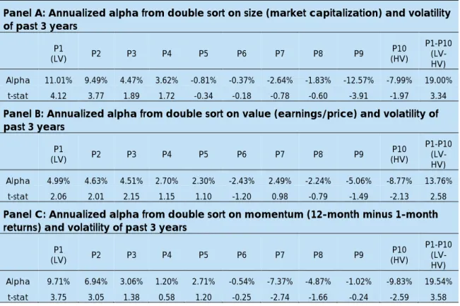
Alpha for top-decile volatility portfolio after controlling for size effect is 11.01%, which is considerably higher and statistically more significant than top-decile volatility portfolio alpha of 7.91% without controlling for other effects. Looking at this outcome and keeping in mind that in our sample we have evidence for size effect, ideally, double sorted alpha must be lower if low volatility portfolio is dominated by a large number of small stocks. Instead, we see the exactly opposite, where low volatility portfolio alpha controlled for size effect is economically and statistically more significant than alpha without controlling for size effect. It implies that low volatility portfolio has agreater proportion of large stocks rather than small within each size-sorted decile portfolio; if at all such minute observation is worth anything. Bottom-decile of volatility portfolio has an alpha of -7.99% after controlling for size. This is slightly smaller than -8.72% without controlling for size effect. It shows that controlling for size does not lead to any improvement in performance of high volatility portfolio. Going by the results, we confirm that volatility effect is independent of size effect.
23
Table 4:
Double-sorted results controlling for other effects
Table 4 reports the annualized alpha and corresponding t-value for volatility decile portfolios after controlling for other effects like size, value and momentum. Panel A, panel B and panel C reports results for size, value and momentum effects respectively. This analysis enables us to detangle the alpha of volatility sorted portfolios from alphas of size, value and momentum factors.
Panel A: Annualized alpha from double sort on size (market capitalization) and volatility of past 3 years
(LV) P1 P2 P3 P4 P5 P6 P7 P8 P9 (HV) P10 P1-P10 (LV-HV) Alpha 11.01% 9.49% 4.47% 3.62% -0.81% -0.37% -2.64% -1.83% -12.57% -7.99% 19.00%
t-stat 4.12 3.77 1.89 1.72 -0.34 -0.18 -0.78 -0.60 -3.91 -1.97 3.34
Panel B: Annualized alpha from double sort on value (earnings/price) and volatility of past 3 years
(LV) P1 P2 P3 P4 P5 P6 P7 P8 P9 (HV) P10 P1-P10 (LV-HV) Alpha 4.99% 4.63% 4.51% 2.70% 2.30% -2.43% 2.49% -2.24% -5.06% -8.77% 13.76%
t-stat 2.06 2.01 2.15 1.15 1.10 -1.20 0.98 -0.79 -1.49 -2.13 2.58
Panel C: Annualized alpha from double sort on momentum (12-month minus 1-month returns) and volatility of past 3 years
(LV) P1 P2 P3 P4 P5 P6 P7 P8 P9 (HV) P10 P1-P10 (LV-HV) Alpha 9.71% 6.94% 3.06% 1.20% 2.71% -0.54% -7.37% -4.87% -1.02% -9.83% 19.54%
t-stat 3.75 3.05 1.38 0.58 1.20 -0.25 -2.74 -1.66 -0.24 -2.59 3.58
Alpha of top-decile volatility portfolio after controlling for value effect is 4.99% compared to 7.91% without controlling for value effect. It is still economically and statistically significant. Corresponding alphas for bottomdecile volatility portfolios are -8.77% and -8.72%. A positive alpha of top-decile volatility portfolio and negative alpha of bottom-decile volatility portfolio are sizeable and significant both in economic and statistical terms. This proves that volatility effect is not value effect but clearly an independent distinct effect than classic value effect.
Alpha of top-decile volatility portfolio after controlling for momentum effect is 9.71% compared to 7.91% without controlling for momentum effect. Corresponding alphas for bottom-decile volatility portfolios are -9.83% and -8.72%. A positive alpha of top-decile volatility portfolio and negative alpha of bottom-decile volatility portfolio are greater than volatility decile alphas and more significant both in economic and statistical terms. In a nutshell, volatility effect is not even momentum effect but an independent effect. The volatility effect remains economically and statistically significant even after controlling for all well-known effects including size, value and momentum.
24
4.3 Robustness Tests
Table 1 reports main results of univariate analysis for the volatility sorted decile portfolios. Top two decile portfolios (P1 and P2), consisting of lower volatility stocks, report significant above average returns. Such outperformance over universe portfolio loses steam and turns into significant underperformance as we move towards bottom decile portfolios (P9
We report the results of the robustness tests to further substantiate our results. First robustness test involves using beta as a measure of risk. We calculate beta for each stock using equally weighted index (EWI) as a proxy to the market portfolio. We then report here the results of comparison between CAPM alphas for portfolios sorted on standard deviation and beta. Second robustness test involves sorting stocks on volatility after controlling for beta using double-sorting to evaluate whether volatility effect and beta effect represent the same effect comparing magnitude and strength of both.
4.3.1 Beta as a Measure of Risk
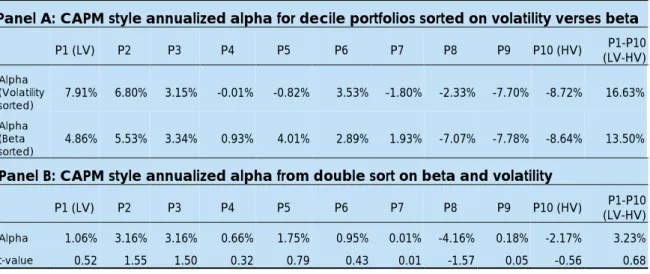
Panel A of Table 5 shows alpha comparison based on portfolios sorted on volatility vs. beta. There is a clear beta effect similar to volatility effect discussed earlier but lesser magnitude.
Panel B of Table 5 shows results of double-sorted decile portfolios, first on beta and then on volatility such as to control beta effect in decile portfolios. The results show that large chunk of alphas disappears and alphas don’t remain statistically significant. However, going by numbers, there is still a clear trend. In closing, we summarise that market misprices systematic risk decile and to some extent idiosyncratic risk too but a large chunk of volatility effect is a beta effect. This is explicable, since, by design, our universe eliminates small stocks, which have greater idiosyncratic volatility and lottery-like payoffs. Besides, our choice of the equally weighted universe as a proxy of the market portfolio makes our beta more representative of total volatility itself. These combined effects dwarf the idiosyncratic volatility effect as reported by other studies.
4.3.2 Sub-period Analysis
We perform sub-period analysis to see if low volatility strategy outperforms only during turbulent times and underperforms during an upward trending market. The period of January 2001 to December 2007 saw a secular bull run in global markets including India before the start of a reversal from January 2008. We check results of volatility decile portfolios with respect to benchmark Nifty 200 in a period from January 2004 to December 2007.We find absolute returns of low-volatility portfolio similar to that of Nifty 200 but at much lower risk measured by annualised standard deviation. Consequently, Sharpe ratio is considerably higher. In fact, LV portfolio delivers marginal outperformance even in the period of secular bull-run in the study.
25
Table 5:
Robustness Test using Beta as Risk Measure
Table 5 reports the results of robustness test using beta as a measure of risk. For the readability, we have reported the alpha for the volatility sorted decile portfolios from Table 1 again here in Panel A for comparison with the beta analysis. Panel B reports alpha for the volatility sorted decile portfolios after controlling for beta see the relative strength of volatility effect as well as beta effect.
Panel A: CAPM style annualized alpha for decile portfolios sorted on volatility verses beta
P1 (LV) P2 P3 P4 P5 P6 P7 P8 P9 P10 (HV) (LV-HV) P1-P10 Alpha (Volatility sorted) 7.91% 6.80% 3.15% -0.01% -0.82% 3.53% -1.80% -2.33% -7.70% -8.72% 16.63% Alpha (Beta sorted) 4.86% 5.53% 3.34% 0.93% 4.01% 2.89% 1.93% -7.07% -7.78% -8.64% 13.50%
Panel B: CAPM style annualized alpha from double sort on beta and volatility
P1 (LV) P2 P3 P4 P5 P6 P7 P8 P9 P10 (HV) (LV-HV) P1-P10
Alpha 1.06% 3.16% 3.16% 0.66% 1.75% 0.95% 0.01% -4.16% 0.18% -2.17% 3.23%
t-value 0.52 1.55 1.50 0.32 0.79 0.43 0.01 -1.57 0.05 -0.56 0.68
5. Conclusion
In closing, we find clear evidence for volatility effect. A portfolio consisting of low volatility or low beta stocks systematically outperforms benchmark portfolio as well as high volatility or high beta stocks portfolio. This outperformance is not only on risk-adjusted basis but also an absolute basis over a period of our study. We also conclude that volatility effect is separate and significant effect and it is neither timid enough to be ignored nor it is a proxy for other well-known effects such as size, value and momentum. In fact, our low volatility portfolio consists of relatively large and growth stocks rather than small and value stocks. Besides, we conclude that a large part of our volatility effect is the same as beta effect and after controlling for beta we don’t find volatility effect significant. However, even after controlling for the beta, low volatility portfolio retains positive alpha whereas high volatility portfolio retains negative alpha. None of them are significant and therefore we conclude that volatility effect is not due to idiosyncratic risk only as claimed by Ang, et al. (2006). and if at all idiosyncratic volatility effects, it may be adding to volatility effect. Evidence of volatility effect in our sample also rebuts the claim of Bali, et al. (2011) that low-risk anomaly disappears once we eliminate small and illiquid stocks from the sample. Our universe consists of relatively large and liquid stocks only and we still find strong evidence for volatility effect. We also find evidence to conclude that outperformance of low volatility portfolio over benchmark is not concentred during negative markets only. We find all the possible economic, as well as behavioural explanations offered in existing literature for the persistence of low-risk anomaly, are also valid in the Indian context. In addition, we add performance chasing behaviour of mutual fund investors as one of the possible explanation for the low-risk anomaly. We conclude with the claim that low-risk anomaly is very strong and significant anomaly in the history of capital markets and it will stay for a long time unless economic and behavioural reasons as well as the market friction that causes it or it becomes overcrowded investment place and loose its sheen. All these are unlikely to happen at least in the near future.
26
References
Agarwalla, S. K., Jacob, J. and Varma, J. R.(2013). Fama-French and Momentum Factors: Data Library for Indian Market. [Online] Available at:
http://www.iimahd.ernet.in/~iffm/Indian-Fama-French-Momentum [Accessed
2015].
Ang, A., Hodrick, R. J., Xing, Y. and Zhang, X. (2006). The Cross-Section of Volatility and Expected Return. Journal of Finance, 61, 259-299.
Ang, Hodrick, Xing and Zhang (2009). High Idiosyncratic Volatility and Low Returns: International and Further U.S. Evidence. Journal of Financial Economics, 91, 1-23. Baker, M., Bradley, B. and Taliaferro, R. (2013). The Low-Risk Anomaly: A Decomposition
into Micro and Macro Effects. SSRN Journal, 23 January.
Baker, M., Bradley, B. and Wurgler, J. (2011). Benchmarks as Limits to Arbitrage: Understanding the Low-Volatility Anomaly. Financial Analysts Journal, January, 67, 40-54.
Bali and Cakici(2008). Idiosyncratic Volatility and the Cross-Section of Expected Returns. Journal of Financial and Quantitative Analysis, 43, 29-58.
Bali, T. G., Cakici, N. and Whitelaw, R. F.(2011). Maxing out: Stocks as lotteries and the cross-section of expected returns. Journal of Financial Economics, Volume 99, 427-446.
Black, F.(1972). Capital Market Equilibrium with Restricted Borrowing. Journal of Business, July, 4, 444-455.
Black, Jensen and Scholes(1972). The Capital Asset Pricing Model: Some Empirical Tests. In Studies in the Theory of Capital Markets, Volume Michael C. Jensen,79-121. Agarwalla, S. K., Jacob, J. and Varma, J. R.(2013). Fama-French and Momentum
Factors: Data Library for Indian Market. [Online] Available at:
http://www.iimahd.ernet.in/~iffm/Indian-Fama-French-Momentum [Accessed 2015]. Ang, A., Hodrick, R. J., Xing, Y. and Zhang, X.(2006). The Cross-Section of Volatility and
Expected Return. Journal of Finance, 61, 259-299.
Ang, Hodrick, Xing and Zhang(2009). High Idiosyncratic Volatility and Low Returns: International and Further U.S. Evidence. Journal of Financial Economics, 91, 1-23. Baker, M., Bradley, B. and Taliaferro, R. (2013). The Low-Risk Anomaly: A Decomposition
into Micro and Macro Effects. SSRN Journal, 23 January.
Baker, M., Bradley, B. and Wurgler, J. (2011). Benchmarks as Limits to Arbitrage: Understanding the Low-Volatility Anomaly. Financial Analysts Journal, January, 67, 40-54.
Bali and Cakici (2008). Idiosyncratic Volatility and the Cross-Section of Expected Returns. Journal of Financial and Quantitative Analysis, 43, 29-58.
Bali, T. G., Cakici, N. and Whitelaw, R. F. (2011). Maxing out: Stocks as lotteries and the cross-section of expected returns. Journal of Financial Economics, Volume 99, 427-446.
Black, F. (1972). Capital Market Equilibrium with Restricted Borrowing. Journal of Business, July, 4, 444-455.
Black, Jensen and Scholes(1972). The Capital Asset Pricing Model: Some Empirical Tests. In Studies in the Theory of Capital Markets, Volume Michael C. Jensen, 79-121.
Blitz, D., Pang, J. and Vliet, P. V. (2013). The Volatility Effect in Emerging Markets. Emerging Markets Review, Volume 16, 31-45.
Carhart (1997). On Persistence in Mutual Fund Performance. The Journal of Finance, Volume 52, 57–82.
Carvalho, de, R. L., Lu, X. and Moulin, P. (2012). Demystifying Equity Risk-Based Strategies: A Simple Alpha plus Beta Description. Journal of Portfolio Management, 38.
27 Choueifaty, Y. and Coignard, Y. (2008). Toward Maximum Diversification. Journal of
Portfolio Management, 35.
Clarke, R., de Silva, H. and Thorley, S. (2006). Minimum-Variance Portfolio in the U.S. Equity Market. The Journal of Portfolio Management, 33(Fall), 10-24.
Fama, E. F. and French, K. (1992). The Cross-section of Expected Stock Returns. Journal of Finance, 47, 424-465.
Frazzini, A. and Pedersen, L. H. (2014). Betting Against Beta. Journal of Financial Economics, 111, 1-25.
Fu (2009). Idiosyncratic Risk and the Cross-Section of Expected Returns. Journal of Financial Economics, 91, 24-37.
Haugen and Baker (1996). Commonality in the Determinants of Expected Returns. Journal of Financial Economics, 41, 401-439.
Haugen, R. A. and Baker, N. L.(1991). The Efficient Market Inefficiency of Capitalization-weighted Stock Portfolios. Journal of Portfolio Management, 17, 35-40.
Haugen, R. A. and Baker, N. L. (1996). Commonality in the Determinants of Expected Returns. Journal of Financial Economics, 41, 401-439.
Haugen, R. A. and Heins, A. J. (1975). Risk and the Rate of Return on Financial Assets: Some Old Wine in New Bottles. Journal of Financial and Quantitative Analysis, December, 10, 775-784.
Haugen, R. and Baker, N.(2005). The Efficient Market Inefficiency of Capitalisation Weighted Stock Portfolios. The Journal of Portfolio Management, 31(Spring), 82-91. Jobson, J. D. and Korkie, B. M. (1981). Performance Hypothesis Testing with the Sharpe
and Treynor Measures. Journal of Finance, Volume 36, 889-908.
Martellini(2008). Toward the Design of Better Equity Benchmarks: Rehabilitating the Tangency Portfolio from Modern Portfolio Theory. Journal for Portfolio Management, 34(4), 34-41.
Memmel, C. (2003). Performance Hypothesis Testing with the Sharpe Ratio. Finance Letters, Volume 1, 21-23.
Poullaouec, T. (2010). Things to Consider When Investing in Minimum Volatility Strategies. State Street Global Advisors Asset Allocation Research.
Scherer, B. (2011). A Note on the Returns from Minimum Variance Investing. Journal of Empirical Finance, 18, 652-660.
Sharpe, W. (1964). Capital Asset Prices: A Theory of Market Equilibrium under Conditions of Risk. The Journal of Finance, 19, 425-442.
Soe, A. M. (2012). The Low Volatility Effect: A Comprehensive Look. S&P DOW JONES Indices Paper, 1 August.