Fuzzy Depth Based Routing Protocol for
Underwater Acoustic Wireless Sensor Networks
Reza Mohammadi, Reza Javidan, Ahmad Jalili
Department of Computer Engineering and Information Technology, Shiraz University of Technology, Shiraz, Iran R.mohammadi@sutech.ac.ir
Abstract – Underwater Wireless Sensor Networks consist of a variable number of sensors and vehicles that are implemented to perform collaborative monitoring tasks over a given area. However, designing energy-efficient routing protocols for this type of networks is essential and challenging because the sensor nodes is powered by batteries, underwater environment is harsh and propagation delay is long. Most of the existing routing protocols used for underwater wireless sensor networks, such as depth based routing (DBR) protocol use a greedy approach to deliver data packets to the destination sink nodes at the water surface. Further, DBR does not require full-dimensional location information of sensor nodes. Instead, it needs only local depth information, which can be easily obtained with an inexpensive depth sensor that can be equipped in every underwater sensor node. DBR uses smaller depth as the only metric for choosing a route. This decision might lead to high energy consumption and long end to end delay which will degrade network performance. This paper proposes an improvement of DBR protocol by making routing decisions depend on fuzzy cost based on the residual energy of receiver node in conjunction with the depth difference of receiver node and previous forwarder node and the number of hops traveled by the received packet. Our simulation was carried out in Aqua-sim an NS2 based underwater Aqua-simulator and the evaluation results show that the proposed fuzzy multi metric DBR protocol (FDBR) performs better than the original DBR in terms of average end to end delay, packet delivery ratio and energy saving.
Index Terms – Underwater wireless sensor networks, Routing protocols, Fuzzy logic, Depth based routing.
I. INTRODUCTION
Wireless sensor networks have been used extensively in many land-based applications. For the past several years, there has been a rapidly growing trend towards the application of sensor networks in underwater environments as it has attracted the interest of many researchers. Underwater Sensor Network will enable a wide range of aquatic applications such as mine reconnaissance, distributed tactical surveillance, water quality monitoring, pollution monitoring, offshore exploration, environmental monitoring and disaster prevention [1][2][3].
Underwater wireless sensor networks are significantly different from terrestrial wireless sensor networks. The adverse environmental conditions pose a range of challenges to underwater networking and communication. The first challenge is that the radio channels do not work well under water, although the acoustic signal is considered as the only feasible medium that works satisfactorily in underwater environments. Further, the use of acoustic channels results in high channel error rates, long propagation delays (approximately 1500 m/s) and low communication
bandwidth. Secondly, the underwater wireless sensor nodes are highly dynamic because underwater wireless sensor nodes are mobile and may move with water currents. Thirdly, underwater wireless sensor nodes are powered by battery. In this case, power of the sensor node is limited and usually batteries cannot be easily recharged or changed when depleted [4][5][6].
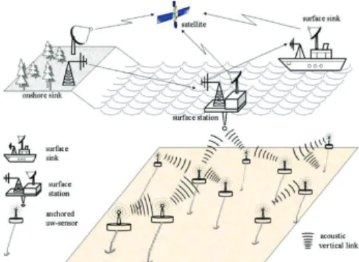
Figure 1 shows the architecture of an underwater wireless sensor network. According to Figure 1, underwater sensors gather environmental phenomena and send the collected data to other sensors using acoustic signals. Then, these data are routed to surface station. Finally, the surface station sends the collected data to onshore sink node [7].
Figure 1: Architecture of 3D underwater wireless sensor network [7]
In the underwater wireless sensor networks, the main role of the routing protocols are discovering and maintaining the routes. Due to the different characteristics of the underwater applications and environment, terrestrial routing protocols are not suitable for underwater wireless sensor networks. Therefore, designing energy-efficient, robust and scalable routing protocols in underwater wireless sensor networks is very challenging.
The rest of this paper is organized as follow. In Section II, we discuss some of the previous routing protocols. Then, we present FDBR in detail in Section III. After that, we evaluate the performance of FDBR in Section IV and V. Finally we present the conclusion in Section VI.
II. RELATED WORK
Recently, there has been an extensive research on routing protocols for terrestrial wireless sensor networks since the different characteristics of the underwater applications and environment, and the terrestrial routing protocols are not suitable for underwater wireless sensor networks. Moreover, the unique acoustic communication characteristics such as
limited energy resource, limited bandwidth, and long propagation delay, multipath and fading phenomena and high error rate pose many challenges when applying terrestrial routing protocols in underwater wireless sensor networks. In this section, we review some related work on routing protocols in underwater wireless sensor networks.
VBF (Vector Based Forwarding) is the first geographic based routing protocol designed for mobile underwater sensor networks proposed by Xie et al. [8]. In VBF data packets are forwarded along the routing vector from the source to sink and each node in the network knows its position. In VBF, when a sensor node receives a data packet, it first calculates its distance to the routing vector. If the distance is less than a predefined threshold R, called radius, this node is in the routing pipe and is qualified to forward the packet. To improve the reliability, multiple routes might be used at the same time in VBF. VBF is not suitable for sparse deployment underwater networks and is sensitive about the routing pipe radius threshold.
As we mentioned above, underwater channels have high channel error rates that lead to low reliability. DFR (Directional Flooding Based Routing) proposed by Daeyoup and Dongkyun [9] is expected to increase the reliability of underwater routing. DFR is a packet flooding routing protocol. In DFR, each node in the network knows its position, the location of destination node and the location of one-hop neighbors. In DFR, when a sensor node receives a data packet, it determines dynamically the packet forwarding by comparing the angle between itself and the source, and the destination of packet with a criterion angle, which is included in the received packet. If the angle is less than the criterion angle, this node is qualified to forward the packet.
DBR (Depth Based Routing) proposed by Yan et al. [10] uses a greedy approach to deliver data packets to the destination sink nodes at the water surface. In DBR, each node in the network does not need full dimensional location information and it requires only local depth information of each node. Depth information can be achieved easily with an inexpensive depth sensor compared to full dimensional location information. In DBR, multiple sinks are placed on the water surface. These sink nodes are used to collect the data packets from the underwater sensor nodes. DBR forwards the data packets from deeper sensor nodes to lower depth sensor nodes. In DBR, a sensor node makes its decision on packet forwarding, based on the depth of the previous sender and its own depth. In DBR, when a sensor node receives a data packet, it retrieves depth dpof the packet’s previous hop, which is included in the received packet. Then, it compares dp with its own depth dc. If dp is smaller than dc, then this node is qualified to forward the packet. Otherwise, it discards the packet. Until the data packet reaches at any of the sink node, this process will be repeated. DBR uses redundant packet suppression mechanism to save energy by reducing the number of collisions and preventing other neighboring nodes from forwarding the same packets,. In this approach, when a sensor node receives a packet, it does not send the data packet immediately. Instead, it waits for a certain amount of time, called holding time. After the holding time expires, the node forwards the data packet. At a node, the holding time for a packet is calculated as [10]:
𝑓𝑓(𝑑𝑑) =2𝜏𝜏𝛿𝛿(𝑅𝑅 − 𝑑𝑑), 𝛿𝛿𝛿𝛿(0, 𝑅𝑅] (1)
Where d is the depth difference of receiver node and previous forwarder node, τ is the maximum propagation delay of one hop, R is the maximum transmission range of a sensor node and δ is a parameter that usually equals to R/2. The parameter δ determines the holding time of packets at each node. With a smaller δ, each node has a longer holding time and hence the average end to end delay will be increased. But few nodes will forward the same packet, which results in more energy saving. DBR uses smaller depth as the only metric for choosing a route. This decision might lead to high energy consumption and long end to end delay which will degrade network performance. In the next section, we will propose fuzzy multi-metric DBR protocol that performs better than the original DBR in terms of average end to end delay, packet delivery ratio and energy saving [10].
III. FUZZY SYSTEM FOR FDBR
Fuzzy logic was introduced by Zadeh (1965) as a means of representing and manipulating data that was not precise, but rather fuzzy. Fuzzy logic deals with uncertainty in engineering by attaching degrees of certainty to the answer to a logical question and Fuzzy Logic is a good alternative for many control problems [11]. In contrast to conventional control techniques, fuzzy logic control (FLC) is best utilized in complex ill-defined processes that can be controlled by a skilled human operator without much knowledge of their underlying dynamics. A typical architecture of FLC is shown in Figure 2, which comprises of four principles: a fuzzifier, a fuzzy rule base, inference engine, and a defuzzifier. In fuzzification process, a crisp set of input data are gathered and converted to a fuzzy set using fuzzy linguistic variables, fuzzy linguistic terms and membership functions. After the process of fuzzification, an inference is made based on a set of rules. The fuzzy rule base stores the empirical knowledge of the operation of the process of the domain experts. In the defuzzication step, the resulting fuzzy output is mapped to a crisp output using the membership functions.
Figure 2: Fuzzy logic system
As we mentioned earlier, the value of holding time in DBR affects network performance in terms of energy consumption and average end to end delay. With a longer holding time, the average end to end delay will be increased. On the other hand, with a smaller holding time, the average end-to-end delay is reduced; but less nodes will forward the same packet, which results in more energy saving. To overcome these problems in DBR protocol, we proposed a Fuzzy DBR (FDBR) protocol. The objective of our fuzzy routine is to determine the value of holding time in each sensor node. To calculate the value of holding time, FDBR considers residual energy of receiver node, depth difference of receiver node and previous forwarder node and the number of hops traveled
by the received packet. In the proposed fuzzy system, Mamdani minimum inference method was used as the fuzzy inference method, where the “AND” operation was set to the minimum of the membership functions and “OR” operation was set to the maximum of the membership functions [12]. Defuzzificationwas carried out using center of area Defuzzifier.
The input fuzzy variables are: remaining energy of receiver node, depth difference of receiver node and previous forwarder node and the number of hops traveled by the received packet. The rules for fuzzy inference system are made on the basis of the inputs depth, hop-count and the energy. There is a single output fuzzy variable, namely delay, the defuzzified value of which determines the value of holding time. The membership functions for the input and output variables are shown in Figure 3. As shown in Figure 3, triangle membership functions were used to represent inputs and output, with two linguistic variables to the inputs: Low and High, and three for the output: Low, Medium, and High.
Figure 3(a): Membership function of Depth (meters)
The membership function of Depth input variable defines as: 𝑚𝑚𝑚𝑚𝑚𝑚𝑚𝑚𝑚𝑚𝑚𝑚: { 0 𝑥𝑥 > 100 𝑜𝑜𝑚𝑚 𝑥𝑥 < 0 𝑙𝑙𝑜𝑜𝑙𝑙 =100 0 ≤ 𝑥𝑥 ≤ 100−𝑥𝑥 ℎ𝑖𝑖𝑖𝑖ℎ =100𝑥𝑥 0 ≤ 𝑥𝑥 ≤ 100 (2)
Figure 3(b): Membership function of Energy (Joules)
The membership function of Energy input variable is defined as: 𝑗𝑗𝑜𝑜𝑗𝑗𝑙𝑙𝑚𝑚𝑚𝑚: { 0 𝑥𝑥 > 100 𝑜𝑜𝑚𝑚 𝑥𝑥 < 0 𝑙𝑙𝑜𝑜𝑙𝑙 =−𝑥𝑥20 0 ≤ 𝑥𝑥 ≤ 100 ℎ𝑖𝑖𝑖𝑖ℎ =100𝑥𝑥 0 ≤ 𝑥𝑥 ≤ 100 (3)
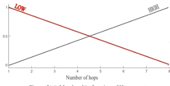
Figure 3(c): Membership function of Hop_count
The membership function of hop-count input variable is defined as: ℎ𝑜𝑜𝑜𝑜𝑜𝑜𝑜𝑜𝑗𝑗𝑜𝑜𝑚𝑚: { 0 𝑥𝑥 > 8 𝑜𝑜𝑚𝑚 𝑥𝑥 < 0 𝑙𝑙𝑜𝑜𝑙𝑙 =−𝑥𝑥8 0 ≤ 𝑥𝑥 ≤ 8 ℎ𝑖𝑖𝑖𝑖ℎ =𝑥𝑥80 ≤ 𝑥𝑥 ≤ 8
(4)
Figure 3 (d). Membership function of Delay
The membership function of delay output variable is defined as: 𝑑𝑑𝑚𝑚𝑙𝑙𝑑𝑑𝑑𝑑: { 0 𝑥𝑥 > 8 𝑜𝑜𝑚𝑚 𝑥𝑥 < 0 𝑙𝑙𝑜𝑜𝑙𝑙 =−𝑥𝑥8 0 ≤ 𝑥𝑥 ≤ 8 ℎ𝑖𝑖𝑖𝑖ℎ =𝑥𝑥80 ≤ 𝑥𝑥 ≤ 8
(5)
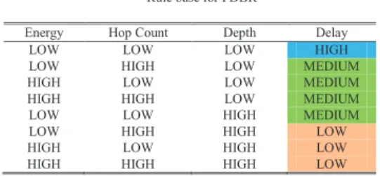
The membership function of depth depends on the maximum transmission of sensor nodes. In Figure 3(a), the maximum transmission of sensor node is assumed at 100 meters. The membership function of residual energy depends on the battery capacity of sensor nodes. In Figure 3(b), the battery capacity of sensor node is assumed at 100 Joules. The membership function of hop count depends on the maximum hop count traveled by the data packets. In Figure 3(c), the maximum hop count is assumed 8 hops.According to the equation (1), we choose the delay in the [0 0.27] range. By assuming R=100 (maximum transmission range) and δ=R/2 in equation (1), if d (depth difference) is set to 0, then the value of delay becomes 0.27, and if d is set to 100, the value of delay becomes 0. As shown in Table 1, the rule base of FDBR consists of 8 rules. In “Delay” column the low, medium and high are linguistic variables. These variables are converted to real values in defuzzification process.
Table 1 Rule base for FDBR
Energy Hop Count Depth Delay LOW LOW LOW HIGH LOW HIGH LOW MEDIUM HIGH LOW LOW MEDIUM HIGH HIGH LOW MEDIUM LOW LOW HIGH MEDIUM LOW HIGH HIGH LOW HIGH LOW HIGH LOW HIGH HIGH HIGH LOW
IV. PERFORMANCE EVALUATION
In this section, we perform a simulation study to validate FDBR. First, we describe details of simulation settings. After explaining metrics of interest, we evaluate how FDBR performs compared to DBR.
A.Simulation Settings
All simulations are performed using the Aqua-Sim [13] an NS2 based underwater simulator. Unless otherwise indicated for a certain experiment, the simulation parameters that we use are as follows. Source node is placed at the center of bottom layer in our experiment. We use Figure (3) membership functions for FDBR. The maximum transmission range is 100 meters (spherical). The interference range is the same as the transmission range. The data generating rate at the source node is 1 pkt/s (one packet per second). The initial energy of each node is 100 joule. We set the size of data packets to 100 bytes. The bit rate is 10 Kbps. The power consumption in receiving, sending and idling mode are 0.3w, 0.6w, and 10mw. For DBR protocol, we set δ parameter to R/2, because according to the [10] when δ=R/2, DBR has better performance in terms of average end to end delay and energy consumption. In our simulations, the same broadcast MAC protocol as in [8] is used.
B.Performance metrics
We define three performance metrics: Total energy consumption, packet delivery ratio and average end to end delay. Average end to end delay is the average time interval from the source to any of the sinks for each successfully delivered packet. Total energy consumption is measured by the energy consumed on idle, transmission and receiving mode of all nodes in the network. The packet delivery ratio is defined as the ratio of the total number of distinct data packets successfully received at the sinks to the total number of packets generated at the source node.
C.Simulation
In the first set of simulations, we study how the number of nodes affects the performance. In this set of simulation, we consider different numbers of sensors randomly deployed in a 500m×500m area. 5 sink nodes deployed at the water surface. This set of simulation last for 1000 seconds and all the results are obtained from the average of 10 runs and a confidence interval of 99% is obtained.
Figure 4(a): Packet Delivery Ratio vs. Number of Nodes
Figure 4 compares DBR and FDBR with respect to the three metrics. Figure 4 (a) shows how the packet delivery ratio changes with different number of nodes. Figure 4 (a) shows that for the different number of nodes, DBR approximately achieves a similar packet delivery ratio to FDBR.
Figure 4(b): Energy Consumption vs. Number of Nodes
Figure 4 (b) shows that FDBR has better energy efficiency compared with DBR. In Figure 4 (b), as the number of nodes increases the difference between FDBR and DBR is clearer.
Figure 4 (c) shows that FDBR has better average end to end delay compared with DBR.
From Figure 4 (b) and Figure 4 (c), we can conclude that FDBR has better performance in terms of average end to end delay and energy saving. This is mainly caused by two factors. First, DBR uses greedy method and does not consider residual energy in sensor nodes which lead to more energy consumption. Second, DBR does not consider the hop count traveled by the data packets, which lead to long average end to end delay. As we mentioned earlier, FDBR considers hop count and residual energy of nodes as well as depth differences which lead to low average end to end delay and more energy saving.
Figure 4(c): Average End to End Delay Vs. Number of Nodes
In the second set of simulation, we study how the mobility of nodes affects the performance. In this set of simulation, we consider 300 numbers of sensors randomly deployed in a 500m×500m×500m area. 5 sink nodes were deployed at the water surface. We assume that the sinks are stationary and the sensor nodes are mobile. Each sensor node randomly selects a direction in 3D environment and moves to the new position with a random speed between the minimal speed 1 m/s and maximal speed, 1 m/s, 3 m/s, 5 m/s, 7 m/s and 9 m/s. This set of simulation last for 1000 seconds and all the results are obtained from the average of 10 runs and a confidence interval of 99% is obtained.
Figure 5 compares DBR and FDBR with respect to the three metrics when the sensor nodes are mobile. Figure 5 (a) shows how the packet delivery ratio changes with mobility of nodes. Figure 5 (a) shows that for the different maximum speed of nodes, FDBR achieves high packet delivery ratio to DBR.
Figure 5 (a): Packet Delivery Ratio vs. Maximum Speed of Nodes
Figure 5 (b) shows that in case of mobility, FDBR has better energy efficiency compared with DBR.Figure 5 (c) shows that in case of mobility, FDBR has lower average end to end delay compared with DBR.
From Figure 5, we observe that the energy consumption, packet delivery ratio, total and average delay do not change much with node speed. The reason is that all routing decisions in FDBR and DBR are made locally. Routing decision in DBR is based on a node’s depth difference information and in FDBR is based on the node’s depth difference information, hop count and residual energy of
sensor nodes. Also Figure 5 shows that when sensor nodes are mobile, FDBR has better performance in terms of packet delivery ratio, average end to end delay and energy saving. This is because unlike DBR, FDBR uses three important parameters to calculate holding time and does not use greedy method to forwarding packets.
Figure 5(b): Energy Consumption vs. Maximum Speed of Nodes
Figure 5(c): Average End to End Delay Vs. Maximum Speed of Nodes
V.
CONCLUSIONSThe paper proposes the use of a fuzzy mechanism for calculating adaptive values for holding time in the DBR protocol. The approach utilizes the hop count of the path and residual energy in sensor node as well as the depth difference to create 3 dimensional rule base for controlling the holding time adaptively. Three performance metrics were used in the performance tests to validate the results. The performance of the proposed scheme was compared with the performance of the original DBR. The performance analysis showed that this fuzzy based multi metric routing has better average end to end delay, packet delivery ratio and energy saving than the original algorithm. For future research study, other metrics can be measured to produce the fuzzy output.
REFERENCES
[1] M. Keshtgari, R. Javidan and R. Mohammadi .” Comparative
Performance Evaluation of MAC Layer Protocols for Underwater
Wireless Sensor Networks”, Canadian Center of Science and
Education, Vol. 6, No. 3; March 2012.
[2] J.-H. Cui, J. Kong, M. Gerla, and S. Zhou. Challenges:Building Scalable Mobile Underwater Wireless Sensor Networks for Aquatic Applications. Special Issue of IEEE Network on Wireless Sensor Networking, May 2006
[3] J. Heidemann, W. Ye, J. Wills, A. Syed, and Y. Li. Research Challenges and Applications for Underwater Sensor Networking. In IEEE Wireless Communications and Networking Conference, Las Vegas, Nevada, USA, April 2006.
[4] V. Hadidi, R. Javidan, A. Hadidi, Designing an Underwater Wireless Sensor Network for Ship Traffic Control, 9th HMSV Symposium, May, 2011, Naples, Italy.
[5] P. Xie and J.-H. Cui,. R-MAC: An energy-efficient MAC protocol for
underwater sensor networks. In Proceedings of International Conference on Wireless Algorithms, Systems, and Applications (WASA), 2007.
[6] R.B. Manjula, S.S. Manvi, Issues in Underwater Acoustic Sensor Networks, International Journal of Computer and Electrical Engineering, vol. 3 n. 1, pp. 101-110, and 2011.
[7] Akyildiz, Ian F., Dario Pompili, and Tommaso Melodia. "Underwater acoustic sensor networks: research challenges." Ad hoc networks 3, no. 3 (2005): 257-279.
[8] Xie, P., Cui, J.-H., Lao, L.: VBF: Vector-Based Forwarding Protocol for Underwater Sensor Networks. In: Proceedings of IFIP Networking 2006, Coimbra, Portugal, and May 2006.
[9] Daeyoup H, Dongkyun K. DFR: directional flooding based routing
protocol for underwater sensor networks. In: Proceedings of the OCEANS; 2008.
[10]Yan H, Shi ZJ, Cui J-H. DBR: depth-based routing for underwater sensor networks. In: Proceedings of the 7th international IFIP-TC6 networking conference on ad hoc and sensor networks, wireless networks, next generation internet. Singapore: Springer Verlag; 2008. [11]Timothy J. Ross, “Fuzzy Logic With Engineering Applications”, 2nd
Ed.Wiley, 2004.
[12]http://www.doc.ic.ac.uk/~nd/surprise_96/journal/vol4/sbaa/report.fuzzy sets.html (August 2012)
[13]PengX,etal.. Aqua-Sim: an NS-2 based simulator for underwater sensor networks. In: Proceedings of the OCEANS2009, MTS/IEEE Biloxi—
marine technology for our future: global and local challenges; International Journal of Computers, Communication and Control, Romania.2009.