Burgess, Alexandra Jacquelyn (2017) The variable light
environment within complex 3D canopies. PhD thesis,
University of Nottingham.
Access from the University of Nottingham repository:
http://eprints.nottingham.ac.uk/38967/1/A%20Burgess%20Final%20Thesis%20Nov %202016.pdf
Copyright and reuse:
The Nottingham ePrints service makes this work by researchers of the University of Nottingham available open access under the following conditions.
This article is made available under the University of Nottingham End User licence and may be reused according to the conditions of the licence. For more details see:
http://eprints.nottingham.ac.uk/end_user_agreement.pdf
THE VARIABLE LIGHT ENVIRONMENT WITHIN
COMPLEX 3D CANOPIES
ALEXANDRA JACQUELYN BURGESS BA (Hons) Oxon
Thesis submitted to the University of Nottingham for the degree of Doctor of Philosophy
i
Abstract
With an expanding population and uncertain consequences of climate change, the need to both stabilise and increase crop yields is important. The relationship between biomass production and radiation interception suggests one target for improvement. Under optimal growing conditions, biomass production is determined by the amount of light intercepted and the efficiency with which this is converted into dry matter. The amount of light at a given photosynthetic surface is dependent upon solar movement, weather patterns and the structure of the plant, amongst others. Optimising canopy structure provides a method by which we can improve and optimise both radiation interception and also the distribution of light among canopy layers that contribute to net photosynthesis. This requires knowledge of how canopy structure determines light distribution and therefore photosynthetic capacity of a given crop species.
The aim of this thesis was to assess the relationships between canopy architecture, the light environment and photosynthesis. This focused on two core areas: the effect of varietal selection and management practices on canopy structure and the light environment and; the effect of variable light on select photosynthetic processes (photoinhibition and acclimation). An image-based reconstruction method based on stereocameras was employed with a forward ray tracing algorithm in order to model canopy structure and light distributions in high-resolution. Empirical models were then applied using parameterisation from manually measured data to predict the effects of variable light on photosynthesis.
The plasticity of plants means that the physical structure of the canopy is dependent upon many different factors. Detailed descriptions of canopy architecture are integral to predicting whole canopy photosynthesis due to the spatial and temporal differences in light profiles between canopies. This inherent complexity of the canopy means that previous methods for calculating
ii light interception are often not suitable. 3-dimensional modelling can provide a quick and easy method to retain this complexity by preserving small variations. This provides a means to more accurately quantify light interception and enable the scaling of cellular level processes up to the whole canopy.
Results indicate that a canopy with more upright leaves enables greater light penetration to lower canopy layers, and thus higher photosynthetic productivity. This structural characteristic can also limit radiation-induced damage by preventing exposure to high light, particularly around midday. Whilst these features may lead to higher photosynthetic rates per unit leaf area, per unit ground area, photosynthesis is usually determined by total leaf area of the canopies, and within this study, the erect canopies tended to have lower total leaf areas than the more horizontal canopies. The structural arrangement of plant material often led to low levels of light within the lower canopy layers which were punctuated by infrequent, high light events. However, the slow response of photosynthesis to a change in light levels meant that these sun flecks cannot be used by the plant and thus the optimal strategy should be geared towards light harvesting and efficient photosynthesis under low light conditions.
The results of this study contribute to our understanding of photosynthetic processes within the whole canopy and provide a foundation for future work in this area.
iii
Publications
In Peer-reviewed Journals
Burgess AJ, Retkute R, Preston SP, Jensen OE, Pound MP, Pridmore TP, and Murchie EH. The 4-dimensional plant: biological implications of wind- induced movement. Frontiers in Plant Science 7:1392
Burgess AJ*, Retkute R*, Pound MP, Preston SP, Pridmore TP, Foulkes MJ, Jensen OE, and Murchie EH (2015) High-resolution 3D structural data quantifies the impact of photoinhibition on long term carbon gain in wheat canopies in the field. Plant Physiology, 169(2): 1192-1204
Retkute R, Smith-Unna SE, Smith RW, Burgess AJ, Jensen OE, Johnson GN, Preston SP, and Murchie EH (2015) Exploiting heterogeneous environments: does photosynthetic acclimation optimize carbon gain in fluctuating light?
Journal of Experimental Botany66: 2437-2447
Burgess AJ, Retkute R, Pound MP, Mayes S, and Murchie EH. Applications of image-based 3D reconstruction and modelling in assessing light interception and productivity in multi-species intercrop systems. Annals of Botany, in press
Pre-published or under review
Pound MP, Burgess AJ, Wilson MH, Atkinson JA, Griffiths M, Jackson AS, Bulat A, Tzimiropoulos G, Wells DM, Murchie EH, Pridmore TP and French AP (2016) Deep Machine Learning provides state-of-the-art performance in image-based plant Phenotyping. Pre-published at bioRxiv doi: http://dx.doi.org/10.1101/053033
iv
Burgess AJ, Retkute R, Chinnathambi K, Randall JWP, Smillie IRA, Carmo-Silva E, and Murchie EH. Sub-optimal photosynthetic acclimation in wheat is revealed by high resolution 3D canopy reconstruction. New Phytologist
Burgess AJ, Herman T, Retkute R and Murchie EH. Is there a consistent relationship between canopy architecture, light distribution and photosynthesis across diverse rice germplasm? Frontiers in Plant Science
Manuscripts
Burgess AJ, Herman T, and Murchie EH. The effect of nitrogen on rice canopy architecture and photosynthesis; assessed using high-resolution reconstruction and modelling.
Burgess AJ, Retkute R, Simpson C and Murchie EH. The effect of fluctuating light on dynamic acclimation of Arabidopsis thaliana.
Book Chapters
Lin BB, Burgess AJ and Murchie EH (2015) Adaptation for climate sensitive crops using agroforestry: case studies for coffee and rice. Chapter 11 in Ong C, Black C and Wilson J. 2nd Eds Tree-Crop Interactions: Agroforestry in a Changing Climate, CABI
Contributing author to Karunaratne, A.S. (2015) (eds) Proso Millet (Panicum miliaceum L.)-Agronomy, Botany, Ecophysiology and Nutrition. Faculty of Agricultural Sciences, Sabaragamuwa University of Sri Lanka, 70140, Belihuloya, Sri Lanka.
v
Acknowledgements
Firstly, I would like to thank my supervisors, Erik Murchie, Sean Mayes, Debbie Sparkes and Festo Massawe, for tuition, support and guidance throughout the course of my PhD.
I would also like to thank: Renata Retkute for helping me with the modelling aspects of my project and assistance with figures; Michael Pound for help with reconstructions and image analysis; John Alcock and Matt Tovey for running the field trials; Jools Marquez for organising the laboratory; Tiara Herman, Hayley Smith, Kannan Chinnathambi, Jamie Randall, CC Foo, Conor Simpson and Lorna Mcausland for assistance with the laboratory and field work and; my internal examiner, Kevin Pyke, for his invaluable advice.
My grateful thanks to my funders, Crops For the Future and the University of Nottingham.
Finally, I would like to thank my family and my fiancé, Toby Townsend, for supporting me throughout my studies and providing inspiration whilst I was
vi
Abbreviations
2D 2 Dimensional
3D 3 Dimensional
4D 4 Dimensional
AGDM Above ground dry matter
ANOVA Analysis of Variance
C Carbon
chl Chlorophyll
CL Constant Light
cLAI Cumulative leaf area index
CO2 Carbon dioxide
Col Columbia (Arabidopsis thaliana accession)
DAS Days after sowing
DAT Days after transplanting
F/ FI Fractional Interception FL Flag leaf FL Fluctuating Light GM Gross margins GS Growth stage H2O Water HI Harvest Index
Jmax Maximum rate of electron transport
K Potassium
LAD Leaf area duration
LAI Leaf area index
LCP Light compensation point
LEC Land equivalence coefficient
LED Light emitting diode
LER Land equivalence ratio
Ler Landsberg erecta (Arabidopsis thaliana accession)
LHC Light harvesting complex
LRC Light response curves
MAGIC Multi-parent advanced generation intercross
N Nitrogen
vii
O2 Oxygen
P Phosphorous
PAR Photosynthetically active radiation
Pmax Maximum photosynthetic capacity
𝑃̅𝑚𝑎𝑥 Maximum photosynthetic capacity if the [fluctuating] light pattern
was replaced by the average irradiance
𝑃𝑚𝑎𝑥𝑜𝑝𝑡 Optimal maximum photosynthetic capacity
PNUE Photosynthetic nitrogen use efficiency
PPFD Photosynthetic photon flux density
PSI Photosystem I
PSII Photosystem II
Rd Dark respiration
RGB Red green blue
RH Relative humidity
ROS Reactive oxygen species
RUE Radiation use efficiency
SF Scaling factor
SF12 Scaling factor at 12:00 h
TPU Triose phosphate utilisation
TSP Total soluble protein
TVC Total variable costs
Vcmax Maximum rate of carboxylation
Ws Wassilewskija-4 (Arabidopsis thaliana accession)
WT Wild type
WUE Water use efficiency
θ Convexity
viii
Table of Contents
Abstract……… i Publications……….…. iii Acknowledgments……… v Abbreviations………... vi List of Figures……….. xv List of Tables……… xx Chapter 1: Introduction……….. 1 1.1 Research Context……… 11.2 Photosynthesis and Biomass Production……… 3
1.3 The Canopy Light Environment and Architectural Characteristics... 13
1.3.1 Canopy Architecture………... 15
1.3.1.1 Architectural Features……….. 16
Leaf Area……… 16
Clumping……… 17
Leaf Shape and Size……… 19
Leaf Inclination and Orientation………. 20
Leaf Movement………... 22
1.3.2 Direct versus Diffused Light……….. 23
1.4 Linking Architecture, Photosynthesis and Biomass Production…… 24
1.5 Modelling………... 26
1.5.1 Plant Structural Modelling……….. 26
1.5.2 Light Modelling……….. 29
1.5.3 Plant Process Modelling: empirical versus mechanistic…. 31 1.6 Knowledge Gaps……… 33
Aims and Objectives………. 34
Hypotheses………... 34
Thesis Layout………... 35
Chapter 2: Core Methods and Method Development……….. 36
2.1 The Reconstruction Process………... 36
2.1.1 Imaging……….. 38
Canopy Imaging: Imaging in situ………... 38
Single Plant Imaging……….. 38
2.1.2 Reconstructions……….. 39
ix
2.1.2.2 Surface Estimation……….. 41
2.1.2.3 Canopy Formation……….. 47
2.2 Reconstruction Method Development……… 49
2.2.1 Reconstruction Optimisation……….. 49
2.2.2 Optimisation on the Artificial Dataset……… 50
2.3 The Canopy Light Environment: Ray Tracing………... 57
PART I: THE EFFECT OF CROP CHOICE AND AGRONOMIC PRACTICES ON CANOPY PHOTOSYNTHESIS………. 59
Chapter 3: Methods for exploring the light environment within multi-species cropping systems (intercropping)……….. 61
Paper Details………. 61
Abstract………. 62
Introduction……….. 63
Materials and Methods………. 69
Plant Material……….. 69
Imaging and Ray Tracing……… 69
Gas Exchange……….. 71
Ceptometer………... 72
Statistics………... 72
Modelling………. 72
Results……….. 75
Validation of imaging and modelling...………... 75
The Light Environment………... 76
Assessing Productivity……… 80
Discussion………. 84
High-resolution digital reconstruction as a method to explore the intercrop light environment………... 84
Studying light interception in heterogeneous canopies………... 90
Designing the optimal intercropping system………... 92
Concluding remarks………. 94
Supplementary Material………... 96
Chapter 4: The relationship between canopy architecture and photosynthesis………….………. 102
Paper Details………. 102
Abstract………. 103
x
Materials and Methods………. 107
Plant Material and Growth……….. 107
Physiological Measurements………... 108
Imaging and Ray Tracing……… 108
Gas Exchange……….. 109 Statistical Analysis……….. 110 Modelling……….... 110 Results……….. 114 Architectural Features……….. 114 Light Environment ……….. 118 Photosynthesis………. 120 Discussion………. 126
The relationship between canopy architecture and photosynthesis………. 127
Supplementary Material……..………. 133
Chapter 5: The effect of wind-induced movement on light patterning and photosynthesis……….. 138
Paper Details………. 139
Abstract………. 139
Introduction……….. 140
Materials and Methods………. 144
Growth of rice plants………... 144
3D Reconstruction and Modelling………... 144
Results……….. 148
Constant Displacement……… 148
Dynamic Displacement……… 152
Discussion………. 156
Mechanical canopy excitation: a means to manipulate photosynthesis? ………... 157
The technology required for simulating the 4-dimensional canopy……….. 160
Supplementary Material………... 165
Chapter 6: The effect of nitrogen on rice growth, development and photosynthesis……….. 166
Paper Details………. 167
xi
Introduction……….. 168
Nitrogen, canopy architecture and photosynthesis……….. 169
Materials and Methods………. 173
Plant Material and Experimental Design...……….. 173
Physiological Measurements………... 173
Reconstruction and Ray Tracing……….……… 174
Gas Exchange……….. 175 Statistical Analysis……….. 176 Modelling……….... 176 Results……….. 179 Physiological Measurements……….. 179 Photosynthesis……… 187 Discussion………. 191
Use of modelling approaches within nutrient or stress studies... 191
The effect of N availability on crop physiology……….. 193
Concluding Remarks……… 196
Supplementary Material………... 197
PART II: THE EFFECT OF VARIABLE LIGHT ON PHOTOSYNTHETIC PROCESSES ……… 202
Chapter 7: Modelling the effect of photoinhibition in a wheat canopy…….. 204
Paper Details………. 205
Abstract………. 205
Introduction……….. 206
Materials and Methods………. 210
Plant Material...……….……….. 210
Imaging and Ray Tracing…….………... 211
Leaf angle, dry weight and leaf area measurements……… 212
Field Data: Gas Exchange and Fluorescence……….. 212
cLAI and the light extinction coefficient…………..………….. 213
Model Set Up..……….... 214
Results……….. 219
The light environment in a leaf canopy………... 219
Incorporating physiological measurements into the Photoinhibition Model………. 225
Effect of photoinhibition on carbon gain: model output………. 228
xii
High-Resolution digital reconstruction of field-grown plants as
a unique tool……… 233
Accounting for carbon loss at the whole-canopy level………… 235
Managing and mitigating photoinhibition………... 237
Conclusion……… 239
Supplementary Material………... 240
Chapter 8: Modelling the effect dynamic acclimation on photosynthesis.…. 248 Paper Details………. 248
Abstract………. 249
Introduction……….. 250
Materials and Methods………. 255
Theoretical Framework………... 255
Experimental Data………... 256
Model Parameterisation………... 257
Results……….. 259
Quasi-steady net photosynthetic rate………... 259
Light pattern: alternation between two light levels………. 261
Influence of the light intensity switching period………. 263
Fluctuating light……….. 264
Comparison with experimental data……… 265
Discussion………. 267
Conclusion……… 271
Supplementary Material………... 272
Chapter 9: The effect of fluctuating light on acclimation in Arabidopsis thaliana………. 274
Paper Details………. 274
Abstract………. 275
Introduction……….. 276
Materials and Methods………. 280
Plant Growth……… 280
Physiological Measurements………... 281
Gas Exchange……….. 282
Statistical Analysis……….. 283
Curve fitting and Modelling……… 284
Results……….. 286
xiii
Light response curves……….. 286
Chlorophyll Assays………. 288
Response of Photosynthesis to a change in irradiance………… 290
Acclimation Model……….. 292
Discussion………. 295
Supplementary Material………... 300
Chapter 10: Whole Canopy Acclimation……….. 304
Paper Details………. 304
Abstract………. 305
Introduction……….. 306
Materials and Methods………. 310
Experimental and Modelling Strategy……… 310
Plant Material...………... 310
Plant Physical Measurements……….. 310
Imaging and Ray Tracing……….………... 311
Gas Exchange and Fluorescence...……….. 312
Rubisco Quantification.……….. 313
Modelling……….... 314
Results……….. 317
The Canopy Light Environment……….. 317
Effect of Light Levels on Acclimation: Model Output………... 323
Discussion……… 332
Influence of canopy architecture on acclimation………. 332
Implications in terms of nutrient budgeting……….... 335
Concluding Remarks………... 337
Supplementary Material………... 338
Chapter 11: Discussion………... 342
Limitations to work presented in this thesis………. 11.1 Improving Agricultural Productivity……… 344 345 The Yield Gap………. 345
11.1.1 Targets for Improvement arising from this thesis……… 347
Creation of site and situation specific cultivars………... 347
11.1.2 Genetic Improvement of Crop Plants………... 349
11.1.2.1 Genetic manipulation of canopy architecture... 349
xiv
11.1.3 Underutilised Crops……….. 356
11.1.4 Cropping Systems and Management Practices…………. 356
Sustainability……….. 357
Resilience……… 358
11.2 The use of plant reconstruction and modelling techniques in studies of crop processes and productivity………... 359
Applicability of techniques for other situations………. 360
Applicability of techniques for use in developing countries………. 361
11.2.1 Problems with modelling methods………... 362
11.2.2 Improvements to the reconstruction and modelling techniques……… 364
Improvements to the reconstruction technique………... 364
Improvements to the modelling technique………. 365
11.3 The Future of Canopy Research……….. 367
11.4 Concluding Remarks……… 368
REFERENCES……… 369
APPENDICES………. 424
Appendix I……… 425
xv
List of Figures
Figure Legend Page No.
Chapter 1
1.1 Example light response curves as denoted by the non-rectangular hyperbola indicating the shaping parameters.
4
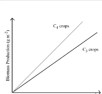
1.2 Example light response curves from a C3 versus C4 leaf. 6 1.3 Example light response curves from a sunlit versus shaded leaf. 9
1.4 Example light response curves from uninhibited versus a photoinhibited leaf.
11
1.5 Example light response curves of a population of photosynthetic cells (i.e. a leaf or a whole canopy).
13
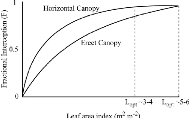
1.6 Fractional interception for a horizontal versus an erect canopy and their optimal LAI.
17
1.7 The effect of leaf dispersion and leaf area index on light transmission.
19
1.8 Exponential decay of light through a horizontal versus an erect canopy.
21
1.9 The determinants of canopy productivity. 24
1.10 The effect of leaf angle and canopy structure on photosynthesis with relation to the light response curve.
25
1.11 Overview of plant modelling approaches. 28
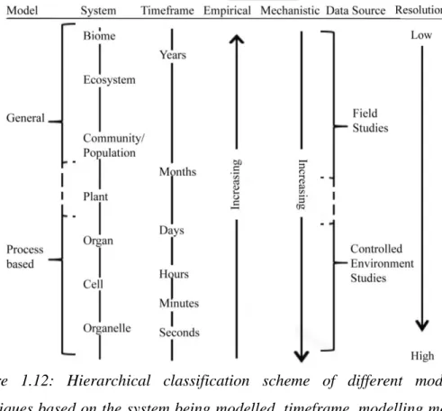
1.12 Hierarchical classification scheme of different modelling techniques based on the system being modelled, timeframe, modelling method data source and resolution.
32
1.13 Types of models, data requirements and their approximate running times.
32
Chapter 2
2.1 Flow diagram showing the general overview of the stages of plant modelling used within this thesis
37
2.2 Set up of the imaging studio for single plant imaging. 39
2.3 Output of VisualSFM indicating the automatically calculated camera positions and corresponding photographs surrounding the target plant
40
2.4 The effect of altered threshold settings (parameters in VisualSFM) on the output point clouds of the same rice plant
xvi
2.5 Segmentation of a point cloud into clusters. 42
2.6 The effect of altered parameters (given in Table 2.1) on the resulting output mesh of a given section of leaf.
45
2.7 Overview of the imaging process for different crops (A) Wheat, (B) Proso Millet, (C, D) Bambara Groundnut (50 DAS, 80 DAS respectively).
46
2.8 Example of a fully reconstructed intercrop canopy of Proso millet and Bambara groundnut with a 3:1 orientation.
48
2.9 Effect of altered boundary sample rate on the output mesh. 49
2.10 Source of light rays in fastTracer3. 57
2.11 Simulated light components (from fastTracer3) over the course of the day for a single point within a canopy.
58
Chapter 3
3.1 Theoretical example of light transmission through a monocropped canopy versus an intercrop canopy.
65
3.2 Validation of light interception in a sole Bambara Groundnut canopy.
75
3.3 Representative reconstructed canopies with the maximum PPFD ranges colour coded for 12:00 h.
77
3.4 Frequency of PPFD values according to the fraction of surface area received at the top layer within each canopy.
78
3.5 Modelled total canopy light interception over the course of the day for different intercrop treatments and respected sole crops.
79
3.6 Example light response curves. 81
3.7 Modelled predicted carbon gain over the course of the day for different intercrop treatments and respected sole crops.
83
3.8 Reconstruction time course of a 3:1 (Bambara groundnut: Proso millet) intercrop canopy development.
89
S3.1 Photograph of the 2:2 (Bambara groundnut: Proso millet) intercrop treatment in the FutureCrop Glasshouse facilities, University of Nottingham, Sutton Bonington Campus, UK.
96
S3.2 Example overview of the Reconstruction Process. 97
S3.3 Example of a full Intercrop Canopy Reconstruction; 3:1 Row layout.
98
S3.4 The relationship between LAI and total PPFD per unit leaf surface area along a row.
xvii
S3.5 Component contribution to leaf area index (LAI) and total intercepted photosynthetic photon flux density (PPFD).
100
S3.6 Frequency of light levels as a function of the fraction of the total surface area of the canopy received at 1200 h by the different treatments.
101
Chapter 4
4.1 Plant height over the course of the experiment, calculated as the average of 5 measurements per plot.
116
4.2 Modelled cLAI, the area of leaf material (or mesh area) per unit ground as a function of depth through the canopy.
117
4.3 Modelled leaf inclination angles throughout depth in the canopy. 118
4.4 Modelled fractional interception as a function of depth in the canopy at 12:00 h.
119
4.5 Whole canopy acclimation model output. 124
S4.1 Example of a time-weighted light pattern at τ=0.2 relative to a non-weighted line.
137
Chapter 5
5.1 Overview of solid body rotation distortion method. 145
5.2 Changing light patterns due to simulated Easterly wind. 148
5.3 Frequency of PPFD values according to the fraction of surface area received at by the central plant in the canopy.
151
5.4 Angle distribution relative to vertical. 152
5.5 Changes as a result of dynamic movement at three time points throughout the day.
155
S5.1 Movie: Change in overall canopy light distribution due to an Easterly wind at 12:00 h between 0-10° distortion.
165
S5.2 Light response curves used to calculate canopy carbon gain. 165
Chapter 6
6.1 Whole canopy reconstruction developmental timecourse. 180
6.2 Physiological Measurements of individual lines. 181
6.3 Depth distributions of leaf material and light interception. 185
6.4 Averaged light as a fraction of surface area in the top third of each canopy at 12:00 h.
186
6.5 (A) Change in SPAD over time. (B) Chlorophyll content analysis 187
6.6 Modelled predicted carbon gain per unit leaf and ground area for each growth stage.
xviii
S6.1 Change in rice production in South East Asia versus Malaysia. 199
S6.2 Trends in Nitrogen fertiliser production, import, export and consumption dynamics in Malaysia.
199
S6.3 Distance between major veins in each of the treatments. 200
S6.4 Depth distributions of leaf material and light interception for all growth stages.
201
Chapter 7
7.1 Stages of the reconstruction of a single plant from multiple color images.
220
7.2 Wheat canopy reconstructions. 221
7.3 Properties of each canopy. 222
7.4 Diagrams depicting the heterogeneity of light environment of the three contrasting wheat canopies.
223
7.5 Experimental validation of the predicted light levels. 224
7.6 Simplified overview of the modeling method. 225
7.7 Data used for the parameterisation of the photoinhibition model. 226
7.8 Results of the model: the predicted effect of photoinhibition on carbon gain
229
7.9 Graph indicating the frequency of light levels received at midday 232
S7.1 Angle distributions within the canopy 240
S7.2 Values of the maximum photosynthetic capacity for each layer were obtained from fitted Light Response Curves.
241
S7.3 Changes in scaling factor over the course of the day for the top and middle layers.
242
S7.4 Fractional interception as a function of cumulative LAI. 243
S7.5 Frequency of PPFD values according to the fraction of surface area received at the top layer at different times during day.
233
Chapter 8
8.1 Net photosynthetic rate as a function of PPFD (light intensity L) and Pmax.
260
8.2 Photosynthetic acclimation under alternation between two light levels.
262
8.3 Influence of the light switching period, S, and time-weighted average timescale, τ, on 𝑃𝑚𝑎𝑥𝑜𝑝𝑡
263
8.4 Predicted Pmax as a function of τ for a typical diurnal variation in
PPFD.
xix
8.5 Comparing model predictions with experimental data. 266
S8.1 (A) Quasi-steady net photosynthetic rate model. (B) Analysis of light intensity regime under alternation between two light levels. (C) Small amplitude light fluctuations.
272
Chapter 9
9.1 Light patterns used for the analysis of dynamic acclimation in Arabidopsis thaliana.
281
9.2 Rosette area timecourse. 287
9.3 Light response curves for plants grown under constant light versus fluctuating light.
288
9.4 Chlorophyll analysis of plants. 289
9.5 Response of Photosynthesis to light level in the days following a change in the light pattern.
291
9.6 Acclimation Model output. 294
S9.1 Normalised response photosynthesis to a change in irradiance in the days following a change in the light pattern.
300
S9.2 Light motif taken from the fluctuating light pattern. 301
S9.3 Example of a time-weighted light pattern at τ=0.3 relative to a non-weighted line (i.e. τ=0).
301
Chapter 10
10.1 Overview of the Reconstruction Process. 317
10.2 Example Canopy Reconstructions from front and top down views. 318
10.3 Progressive lowering of the canopy position in a canopy. 321
10.4 Experimental validation of the predicted light levels. 322
10.5 Fitted Light response curves. 323
10.6 Whole canopy acclimation model output versus gas exchange measurements.
325
10.7 Relationships between photosynthesis and Rubisco properties. 331
S10.1 Diurnal Dynamics of Fv/Fm over the whole day. 338
S10.2 Example of a time-weighted light pattern at τ=0.3 relative to a non-weighted line (i.e. τ=0).
339
S10.3 Model output versus gas exchange measurements. 340
S10.4 Whole canopy acclimation model output versus gas exchange measurements.
xx
List of Tables
Table Legend Page No.
Chapter 2
2.1 Details and default values of parameters in the Reconstructor software.
43
2.2 Simulated reconstruction features in terms of the parameters used with outputs of the total number of triangles, mesh area and difference relative to the ground truth model.
52
2.3 Simulated reconstruction features in terms of the parameters used with outputs of the Hausdorff distance between each mesh, true Hausdorff distance and the resulting percentage difference relative to the ground truth model.
55
Chapter 3
3.1 Total leaf area index (LAI) for each of the treatments. 80
Chapter 4
4.1 Canopy reconstructions and description. 115
4.2 Parameters taken from ACi curve fitting. 120
4.3 Chlorophyll content and ratio at GS2 (85 DAT). 121
4.4 Maximum quantum yield of PSII (Fv/Fm) measured after 20 minutes dark adaptation.
121
4.5 Gas exchange and modelling results at each growth stage. 123
4.6 The relationship between canopy architectural traits and photosynthesis.
127
S4.1 Agronomic details on the 16 Parental Lines used to develop the indica and japonica MAGIC Populations.
133
S4.2 Physiological characteristics of the 15 parental MAGIC lines + IR64 used in the initial screening.
135
Chapter 5
5.1 Daily carbon gain per unit leaf area and total canopy light interception for each of the simulated wind directions.
150
xxi
6.1 Plant Height at each of the studied growth stages. 182
6.2 Dry weight measurements. 183
6.3 Pmax values taken from fitted LRCs at GS5. 188
6.4 Parameters taken from ACi curve fitting. 190
S6.1 Stomatal Physiology. 197
S6.2 Pmax values taken from fitted LRCs, used to calculate canopy carbon gain.
197
S6.3 Canopy K Values 198
Chapter 7
S7.1 Leaf angle for measured versus reconstructed canopies. 245
S7.2 Reconstruction and Canopy Details. 245
S7.3 Leaf versus stem area for measured and reconstructed canopies. 245
S7.4 Symbol Definitions 246
Chapter 8
8.1 Symbol definitions 258
Chapter 9
S9.1 Normalised photosynthesis at stages 1-4 and 6 and the time taken to achieve a normalised photosynthesis.
302
Chapter 10
10.1 Physical canopy measurements of each Line. 319
10.2 Plant and canopy area properties. 320
10.3 Parameters taken from curve fitting. 327
10.4 Rubisco, total soluble protein and chlorophyll content plus chlorophyll a:b and Rubisco: chlorophyll ratios with each layer through the canopy at the postanthesis stage.
1
Chapter 1: Introduction
1.1 Research Context
With an expanding population, conflicting demands for land use and uncertain consequences of future climate change, pressure is placed upon both stabilising and improving crop yield. This is confounded by the need to also find alternative sources of energy, particularly if these new sources compete with food production (i.e. growth of crops solely for biofuels as opposed to consumption/multi-use). With few opportunities to increase the amount of cropland available for cultivation worldwide, any such improvements will hinge upon increasing the productivity of our existing cropping systems (Pinstrup-Andersen & Pandya-Lorch, 1994; Moore, 2007; Zhu et al., 2008). However, studies indicate that both management- and genetic-based improvements are not increasing yields sufficiently to keep up with demand in several different regions of the globe (Peltonen-Sainio et al., 2009; Finger, 2010; Gouache et al., 2010; Ray et al., 2012; 2013). By 2050, global agricultural production requires an increase of 60-110% (FAO, 2009; Tilman et al., 2011); a target exacerbated by the need to provide food security for the approximately 795 million people thought to be chronically undernourished (FAO, 2015). Therefore any future improvements will require a concerted effort (both political and scientific) in order to meet demand.
The ability to generate high levels of biomass in a diverse range of agroecological environments will be an important feature and will be necessary to underpin the required yield increases of both food and energy crops. There are a number of lines of evidence to suggest that biomass production is below the theoretical optimum in crop systems (e.g. Ainsworth & Long, 2005; Lobell
et al., 2009; Godfray et al., 2010; Wang et al., 2012), which may be both due to lack of adaptation (i.e. genetic) and environmental constraints. The harvest index (HI: the ratio of grain to above ground dry matter) of our staple crop species is reaching an upper limit (e.g. Shearman et al., 2005; Lorenz et al.,
2 2010) thus future increases in biomass and grain yield will come from an increased in total above ground dry matter (AGDM). This will require improved cropping practices, improved crop species and varietal selection (including emphasis on new, so called “underutilised” crops), matching crops to their growing conditions, and optimisation of agronomic practices.
The relationship between biomass production and radiation interception suggests one method through which we are able to improve crop yield. Under optimal growing conditions, biomass production is determined by the amount of light intercepted and the efficiency with which this is converted into dry matter. For most crops, in the absence of biotic and abiotic stress, the amount of dry matter accumulated is linearly related to the amount of photosynthetically active radiation (PAR) intercepted by green leaf area (Cooper, 1970; Monteith & Moss, 1977). Furthermore, due to the non-linear response of leaf photosynthesis to light, near maximum photosynthetic rates can be achieved at less than 100% maximal sunlight intensity (Hesketh & Musgrave, 1962; Mock & Pearce, 1975). For example, exposing maize leaves to 50% of maximal sunlight available is sufficient to achieve 80% of the maximal photosynthetic rate and even greater values can be seen in C3 plants
(e.g. soybean, cotton, alfalfa and tree species; see Fig. 1 in Mock & Pearce, 1975). Thus two different routes for improvement are possible: maximising the amount of light intercepted or maximising the efficiency with which light energy can be converted into biomass.
Optimising canopy structure provides a method by which we can improve and optimise both radiation interception and also the distribution of light among canopy layers that contribute to net photosynthesis. This requires knowledge of how canopy structure determines light distribution and therefore photosynthetic capacity of a given crop species. Canopy structure refers to the amount and organization of above ground plant organs; including size, shape and orientation (Norman & Campbell, 1989). There is a great diversity in canopy structure across species (Duncan, 1971; Norman, 1980), with each plant community containing a unique spatial pattern of photosynthetic surfaces,
3 partly as a result of plasticity (Nobel et al., 1993). Plant architecture is the key determinant of the microenvironment surrounding the leaves. This includes factors such as radiant flux density, air, soil and leaf temperature, air vapour pressure, soil heat storage, wind speed and interception of precipitation (Ross, 1981; Norman & Campbell, 1989; Nobel, 1991). Therefore knowledge of how canopy structure influences resource capture and plant metabolism is key to understanding energy flux between plants and their environment.
1.2 Photosynthesis and Biomass production
To reach our goal of doubling productivity of agricultural systems we must establish the maximum efficiency of photosynthesis (Zhu et al., 2008). Photosynthesis is the process by which plants use solar energy in order to create dry matter. Green plants use external resources, predominantly light, water, CO2 and nutrients, to drive the production of biomass. The chemical
pathway involves the conversion of water and atmospheric CO2 into
carbohydrates and water in the presence of sunlight (Eq 1).
CO2 + H2O CH2O + O2 (1)
The efficiency of photosynthesis under a certain set of conditions will depend upon the absorption of photons by the plant, the transfer of this energy to reaction centres and its final use in carbon assimilation (Eq 1). Four aspects of light are important for driving photosynthesis and controlling plant growth and development: irradiance, duration, quality and timing (Geiger, 1994). Irradiance determines the rate at which energy is delivered to the reaction centres; duration influences the total energy received during a given period; spectral quality influences the ability to drive carbon sequestration due to the probabilities of absorbing different wavelengths; and timing determines the effectiveness of light in the regulation of various plant processes according to plant development, for example; source – sink effects. PAR refers to the spectral range of solar radiation that can be used by plants; between 400 and 700 nm. This is usually quantified as µmol photons m-2 s-1 and often referred to as the photosynthetic photon flux density; or PPFD, with a quantum of light
4 called a photon. Photons are absorbed by pigment molecules (such as chlorophyll) and the light energy is converted into chemical energy in the form of carbohydrates. The PPFD at each section of leaf, and the total amount of PPFD intercepted, are the key determinants of the rate of CO2 assimilation; and
thus of whole plant photosynthesis (Duncan, 1971; Norman, 1980).
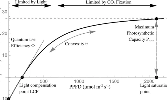
Leaf photosynthesis responds non-linearly to light intensity. Under highly heterogeneous light environments, light intensities will vary from limited to excessive depending on the shape of light response curve. The light response curve may be described by a non-rectangular hyperbola (Eq 2).
𝑃(𝐿, 𝜙, 𝜃, 𝑃𝑚𝑎𝑥, 𝛼)
=𝜙 𝐿+(1+𝛼)𝑃𝑚𝑎𝑥−√(𝜙𝐿+(1+𝛼)𝑃𝑚𝑎𝑥)2−4𝜃𝜙𝐿(1+𝛼)𝑃𝑚𝑎𝑥
2𝜃 − 𝛼𝑃𝑚𝑎𝑥 (2)
The curve relates net photosynthetic rate, P, to PPFD, L. In the absence of light, net photosynthesis will be negative and relate to a dark respiration rate,
RD. It is assumed that the rate of dark respiration is proportional to the
maximum photosynthetic according to the relationship RD = αPmax. The light
response curve can be characterised by three shaping parameters: quantum yield (), convexity (θ) and maximum photosynthetic capacity (Pmax). The
quantum yield refers to the initial linear portion of the curve and describes the maximum efficiency with which light can be used to fix carbon whilst the convexity, or bending factor, describes the curvature. The net photosynthesis rate (P) rises until it reaches a maximum: the maximum photosynthetic capacity (Pmax). The value at which photosynthesis matches respiration (where
net carbon assimilation is equal to zero) is known as the light compensation point. An example light response curve indicating each of the parameters is given in Figure 1.1.
5
Figure 1.1: Example light response curves as denoted by the non-rectangular hyperbola indicating the shaping parameters.
The shape of the light response curve, and thus the values of the shaping parameters, will depend upon the biochemical pathway employed (i.e. C3/C4)
the light absorption properties of the leaf, the relative concentration of the structures involved in light harvesting and the current status of the leaf (Adamson et al., 1991; Chow et al., 1991; Murchie & Horton, 1997; Retkute et al., 2015). There are a number of different processes and pathways that can influence this shape.
The underlying biochemical pathway used to assimilate CO2 can also
determine the productivity of the plant and thus the shape of the light response curve. CO2 can be reduced to carbohydrates via two different carboxylation
pathways. In C3 plants, the Calvin cycle reduces CO2 initially into a 3-carbon
compound whereas in C4 plants a 4-carbon compound is first produced before
entering the Calvin cycle. Differences between the two modes of photosynthesis extend from the biochemical to higher levels of organisation including structural differences such as the cellular organisation in C4 plants
known as “Kranz anatomy”, used to compartmentalise the pathway and concentrate CO2 (Sage & Monson, 1999). These different mechanisms of
Convexity θ Quantum use Efficiency Φ Maximum Photosynthetic Capacity Pmax Light saturation point Light compensation point LCP
Dark Respiration rate RD
Limited by Light Limited by CO2 Fixation
PPFD (μmol m-2 s-1) N et pho tosy nt het ic r at e ( μm ol m -2 s -1 )
6 carboxylation can lead to different photosynthetic productivities. Because C4
plants contain this mechanism for concentrating CO2 within leaves,
photorespiration (the alternative reaction catalysed by Rubisco using O2) is
effectively eliminated, as oxygen is unable to compete with CO2 for the active
binding site of Rubisco. This enables C4 plants to have a higher efficiency than
C3 plants (Gowik & Westhoff, 2011). As well as the biochemical and structural
differences between C3 and C4 plants, they also differ in their response to
external stimuli including rising CO2 levels, temperature and light (Still et al.,
2003). Example light response curves from a C3 versus a C4 plant is given in
Figure 1.2.
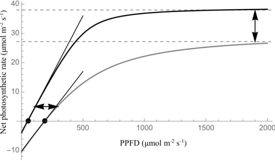
Figure 1.2: Example light response curves from a C3 (grey line) versus C4
(black line) leaf. Arrows denote the differences in the light compensation point and Pmax.
Due to the inherent differences in their photosynthesis and associated water- and nutrient-use efficiencies (WUE and NUE), the advantages of C4
photosynthesis over C3 are maximal under high temperatures, high light
intensities and limited water (Ehleringer & Bjorkman, 1977). As such, C3 crops
are located in most temperature regions whilst C4 plants are typically found in
tropical or semi-tropical habitats, often with high light and temperature conditions and often drought. C3 species include temperate crops, root crops,
PPFD (μmol m-2 s-1) N et pho tosy nt het ic r at e ( μm ol m -2 s -1 )
7 tropical legumes and trees whereas C4 crops include most tropical cereals and
grasses (Azam-Ali & Squire, 2002).
The shape of the light response curve is not fixed, but rather can change as a result of the environmental conditions to which the plant is exposed. The sessile lifestyle of plants necessitates a sophisticated acclimation mechanism to optimise resource capture in a changing environment (Dietzel & Pfannschmidt, 2008). Such mechanisms occur over different time scales to enable plants to adapt to and cope with the variations of light experienced in the natural world; both in terms of light intensity and of spectral quality (Niinemets & Anten, 2009). As the most variable environmental driver light imposes a two-fold challenge; the need to efficiently utilise as many photons as possible whilst simultaneously preventing harm caused by excess radiation. Achieving the optimal balance between these two states is critical to maximise both productivity and mitigate radiation-induced damage (Demmig-Adams et al., 2012).
Two such mechanisms that enable plants to respond to changes in light are acclimation and photoprotection. Acclimation refers to a long term (days) change in the composition and organization of photosynthetic apparatus and leaf morphology (Walters, 2005). Acclimation can be broadly split into two different mechanisms: developmental acclimation and dynamic acclimation. Developmental acclimation refers to changes occurring during leaf development which are largely irreversible whereas dynamic acclimation is the ability for fully developed leaves to change their photosynthetic capacity (Minorsky, 2010). Dynamic acclimation is plastic, fluctuating over timescales of hours to days (Murchie & Horton, 1997). Photoprotection is usually a short-lived process describing the pathways and mechanisms that regulate the absorption and dissipation of light energy which is especially important when chlorophyll absorbs more energy than can be used in photosynthesis (Murchie & Niyogi, 2011). These mechanisms are an integral part of photosynthetic regulation and there is emerging evidence that any alterations to these processes may impact upon the ability of a plant to assimilate carbon over long
8 periods of time; thus affecting biomass production (Külheim et al., 2002; Athanasiou et al., 2010; Murchie & Niyogi, 2011). Such differences in leaf properties are part of a set of integrated mechanisms including biomass partitioning and night-time respiration (Sims & Pearcy, 1994) and their impact can be seen through changes to the light response curve.
Any given acclimation state of a leaf is defined by the maximum photosynthetic capacity (Pmax) value as well as dark respiration (RD) (see Fig.
1.1). There is substantial variation between species in their ability to acclimate, with plants from semi-shaded environments exhibiting the greatest plasticity in acclimation capacity (Murchie & Horton, 1997). This suggests that there are both benefits and costs associated with acclimation. At the whole canopy level, the ability for individual plant leaves to acclimate is also dependent upon leaf age and availability of nutrients (Field, 1981; Pons et al., 2001; Murchie et al., 2002; 2005; Hikosaka, 2005). This inherent plasticity enables foliage photosynthetic potentials to increase with an increasing light availability (e.g. Hirose & Werger, 1987; Thornley, 2004; Johnson et al., 2010). Depending upon the species, photosynthetic capacity can vary between two- and 20-fold from the canopy top to bottom.
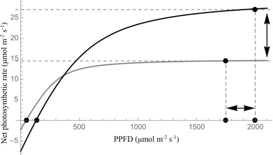
One of the simplest examples of acclimation within a spatial scale can be seen in the anatomical and physiological differences between sun and shade leaves, and is a key example of developmental acclimation. Sun leaves differ from shade leaves primarily in their higher light-saturated rates of photosynthesis (Pmax) (Lambers et al., 2008) and higher dark respiration (RD)
rates (Figure 1.3). Differences in anatomy, which are determined early in development and are largely irreversible, can constrain the potential of leaves to acclimate further (dynamically acclimate) (Murchie et al., 2005). Sun leaves are generally thicker, with differing cellular structure, providing more space for photosynthetic components per unit leaf area, and have thicker palisade parenchyma. Contrary to this, shade leaves are often thinner with a greater surface area, requiring less investment in terms of nitrogen and carbon. Further differences can be seen in the biochemical properties of the two types of
9 leaves; sun leaves contain a greater chlorophyll a: chlorophyll b ratio, larger amounts of Calvin-cycle enzymes, and more components of the electron transport chain (including b6f cytochromes and ATPase). For some plants, the
change in Pmax between different acclimation states shows an almost linear
relationship to an increase in the amount of photosynthetic compounds (Evans & Seemann, 1989), thus investment in compounds that determine photosynthetic capacity translates to higher photosynthetic rate at increased irradiance levels (e.g Anderson., 1995; Evans & Poorter, 2001; Murchie et al., 2002; Walters, 2005). These differences help sun leaves to exploit high irradiances more efficiently. Their ability to regenerate more ATP and NADPH to alleviate the over-reduction of PSII reaction centres at high PPFD helps to minimise their risk of photoinhibition (Chow, 1994; Baker & Oxborough, 2004).
Figure 1.3: Example light response curves from a sunlit (high-light acclimated; black line) versus shaded (low-light acclimated; grey line) leaf.
The ability of preexisting foliage to dynamically acclimate requires a transition from high photosynthetic capacity under high irradiances to high light efficiency under low irradiances and vice versa (Hikosaka & Terashima, 1995). Such a transformation will alter both the total carbon assimilation and the susceptibility to photoinhibition (Baker & Oxborough, 2004). Acclimation to an increased irradiance can include adjustments in both physiological and morphological traits to achieve an increase in amounts of photosynthetic
PPFD (μmol m-2 s-1) N et pho tosy nt het ic r at e ( μm ol m -2 s -1 )
10 components per unit area. The extent of these changes will depend on whether the increase in irradiance occurs before or after leaf development becomes fixed (i.e. before or after leaf expansion) (Turnball et al., 1993; Murchie et al., 2005). Contrary to biochemical changes, morphological features are largely irreversible (Eschrich et al., 1989; Sims & Pearcy, 1992). This may limit complete acclimation to the light environment in some cases (Oguchi et al., 2005; 2003; Tognetti et al., 1998). This is of relevance because the ability of mature leaves to acclimate to changes in irradiances is generally limited to existing chloroplasts and cells and, coupled with gene expression data, requires modification of an existing protein profile.
The resulting effect of acclimation is highly dependent upon the light environment in which the plant is grown. Whilst it is relatively well understood how a plant responds to a change from low to high growth irradiance, or vice versa, response to fluctuating light is less well understood. Furthermore, understanding the response of a collection of photosynthetic cells (i.e. a whole leaf or the whole canopy), is even more complex. The final response will also be dependent upon species or varietal selection, with evidence for species-specific differences in the relative durations of cellular division and expansion during leaf development (Van Volkenburgh, 1999; Stiles & Van Volkenburgh, 2002) and biochemical differences i.e. in chlorophyll contents and ratios, Rubisco amounts, electron transport capacity or enzyme activity (Evans, 1989; Murchie & Horton, 1997; Carmo-Silva & Salvucci, 2013; Carmo-Silva et al., 2015; Orr et al., 2016).
As growth irradiance increases, absorbed photons may become in excess if they are produced quicker than they can be used in photosynthesis (Murchie & Niyogi, 2011). Due to the sensitivity of PSII, high light levels may lead to damage to the photosynthetic apparatus, for example through the production of reactive oxygen species, resulting in a sustained decrease in quantum yield. Plants have an ability to regulate the amount of light they intercept through changes in leaf area, leaf angle (see section 1.3.1) or chloroplast movement, or on a molecular level, through acclimatory adjustments in LHC antenna size
11 (state transitions). However, if excess energy has been absorbed, it can be dissipated via a number of different routes, broadly termed photoprotection. The effect of photoinhibition on shaping parameters of the photosynthesis light response curve is already well characterised (Figure 1.4). The primary effect of photoinhibition is the reduction in Φ, which is important under low light conditions (Powles, 1984; Björkman and Demmig, 1987; Krause and Weis, 1991). However under conditions causing photoinhibition, a reduction in Φ is often accompanied by a similar reduction in θ (Ögren and Sjöström, 1990; Leverenz, 1994).
Figure 1.4: Example light response curves from uninhibited (black line) versus a photoinhibited (grey line) leaf.
Both acclimation and photoprotection represent a subset of regulatory mechanisms used in order to accommodate for variations in light availability, and can be effective in reducing damage due to excess excitation energy. However the different processes will interact together and thus the actual productivity of the plant will depend upon the balance between different states. For example, exposure to excess light levels may lead to the enhancement of photoprotective mechanisms and in turn photoprotection may place an upper limit on the capacity to acclimate (e.g. Sheehy et al., 2000, Demmig-Adams et al., 2012). Optimal plant metabolism would track current environmental
PPFD (μmol m-2 s-1) N et pho tosy nt het ic r at e ( μm ol m -2 s -1 )
12 changes and alter photosynthesis instantaneously (Retkute et al., 2015). However, this does not happen and there is a time lag before the leaf can fully respond to changes (Walters & Horton, 1994; Athanasiou et al., 2010). The length of the time lag will depend upon the process being evoked. For acclimation to a change in light intensity, the time lag for increasing light intensity is longer than that for a decreasing light intensity. This is thought to be due to the protein synthesis, maintenance and investment requirements (in terms of carbon, nitrogen and other resources) for an increased Pmax
(Athanasiou et al., 2010; Retkute et al., 2015).
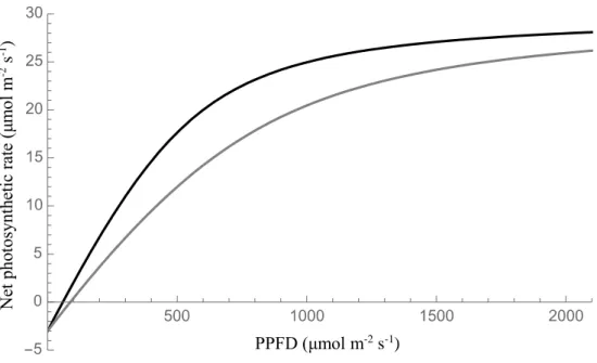
The relationship between light and photosynthesis can also be extended to a population of photosynthesising cells; for example a leaf or a whole canopy. Each section of photosynthetic material on a plant will place somewhere along the light response curve, this can be summed up over the organ or plant and thus build a curve that represents the whole structure. The shape of the resultant curve will depend upon a number of factors including those mentioned above as well as structural characteristics. The variability of light within a whole plant stand and the features of plants that determine these differences are discussed in more detail in the next section (1.3). An example light response curves is given in Figure 1.5. In the case of a canopy, a dense structure that absorbs the majority of light within the top portion of leaf material will have a whole canopy light response curve that rises sharply and then saturates (solid line in Fig. 1.5). However, if light is able to penetrate into deeper canopy layers the shape of the curve will not saturate until higher levels and may not saturate at all. Similarly, at the organ level, thicker leaves lead to a more asymptotic response.
13
Figure 1.5: Example light response curves of a population of photosynthetic cells (i.e. a leaf or a whole canopy). The thicker the population, the more light is absorbed in the upper layers (solid line) whereas a less dense/ thick population absorbs radiation over a greater surface area (dashed line) thus leading to saturation at a higher incident radiation.
1.3 The Canopy Light Environment and
Architectural Characteristics
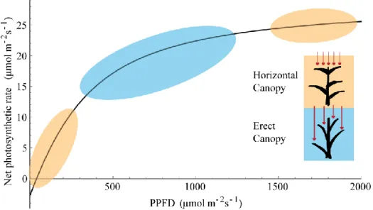
Light availabilities can differ between 20- and 50-fold between the top and bottom within a closed plant canopy (Stadt et al., 1999). Interception depends on a number of different factors including leaf orientation and shape, the spatial arrangement of photosynthetic surfaces (i.e. uniform versus clumping), sun elevation, the finite width of the sun’s disc and changes in spectral distribution of PPFD within the canopy (Nobel et al., 1993). It was discovered that absorption of light by a canopy approximates the absorption of light through a liquid, as described by Beer’s law, particularly when there is a random distribution of leaves (Duncan, 1971; Monsi et al., 1973; Norman, 1980). PPFD (μmol m-2 s-1) N et pho tosy nt het ic r at e ( μm ol m -2 s -1 )
14 When applied to canopies, Beer’s law of exponential decay states that:
𝐼 𝐼𝑜= 𝑒
−𝐾𝐿 (Eq. 3)
where I refers to radiation at a specific point in the canopy, Io refers to radiance
at the top of the canopy, L refers to leaf area index (LAI; the area of leaves per unit area of ground; calculated as the number of plants per unit area multiplied by the number of leaves per plant and the mean area of plant leaf; section 1.3.1) and K is the extinction coefficient for radiation. The extinction coefficient, K, is determined by the angle and orientation of foliage plus its transparency, and is often species or variety specific. Beer’s law shows that as we move vertically down through a canopy, radiation decreases exponentially with the amount of leaf material encountered (Monsi & Saeki, 1953; Monsi et al., 1973) as a function of distribution of leaf area along canopy height and of spatial aggregation and foliage inclination angle (Cescatti & Niinemets, 2004). The radiation is intercepted with depth in the canopy and either reflected or absorbed. This law formed the basis for the first mathematical description of canopy photosynthesis. As canopy characteristics determine the K and L
values, it is important to quantify the architecture of plants.
Variations in light intensity can occur over different spatial or temporal scales. Spatial scales include variation that can be attributed to shading effects within a plant stand, or a single plant canopy, whereas temporal scales may refer to long-term solar radiation changes (for example, as a result of seasonal change) or short-term response such as fluctuating light enforced by sun position, cloud or leaf movement. Therefore the interception of light will depend on a number of different factors including leaf orientation and shape, the spatial arrangement of photosynthetic surfaces (i.e. uniform versus clumping), sun elevation, the finite width of the sun’s disc and changes in spectral distribution of PPFD within the canopy (Nobel et al., 1993). Such variable patterns will lead to periods of time where photosynthesis is fully saturated, and others where photosynthesis may be below or approaching the light compensation point.
15
1.3.1 Canopy Architecture
Plant architecture refers to the spatial organisation of plant organs (Barthelemy & Caraglio, 2007). The resultant structure impacts many processes within the plant including mechanical stability (Moulia et al., 2006; Niklas, 1994), productivity and yield (Khush, 1996; Sakamoto & Matsuoka, 2004), disease and stress resistance (Coyne, 1980; Wolfe, 1985; Jung et al., 1996; Ando et al., 2007; Grumet et al., 2013) and photosynthesis (Song et al., 2013).
Canopy architecture varies greatly both within and between species. The arrangement of plant material, both spatially and temporally, leads to a highly heterogeneous light environment. Canopy photosynthesis depends upon two factors: the distribution of light within the canopy, and the biochemical capacities of the canopy elements (Horton, 2000; Sinoquet et al., 2001; Valladares & Niinemets, 2007; Zhu et al., 2010; Matloobi, 2012). In terms of canopy photosynthesis, the most efficient canopy architecture is that in which all the leaves are evenly illuminated at quantum flux densities which saturate photosynthesis (Valladares & Niinemets, 2007). In other words, optimal utilization of light generally occurs when incident radiation is distributed uniformly across all leaf layers due to the non-linear hyperbolic relationship between photosynthesis and light. The number of leaves that are exposed to radiation levels above that required for positive net photosynthesis (above photosynthetic light compensation but below light saturation) is maximised under these conditions (Clendon & Millen, 1979; Hodanova, 1979; Turitzin & Drake, 1981). Such strategies help to increase the amount of intercepted PAR thus unifying the photosynthetic rates within the canopy by reducing the foliar absorption coefficient of upper leaves and optimizing photosynthetic performance and productivity (Stewart et al., 2003; Cescatti & Niinemets, 2004; Sarlikioti et al., 2011). This may, in part, be due to leaf acclimation to lower light intensities and increased physiological age of leaves in lower canopy layers (Niinemets, 2007). However, this canopy structure is rarely found in nature. More commonly, leaves positioned at the top of the canopy are