Image Caption Generator Based On Deep Neural Networks

(1)

Image Caption Generator Based On Deep Neural Networks

Jianhui Chen CPSC 503 CS Department Wenqiang Dong CPSC 503 CS Department Minchen Li CPSC 540 CS Department Abstract

In this project, we systematically analyze a deep neural networks based image caption generation method. With an image as the in-put, the method can output an English sen-tence describing the content in the image. We analyze three components of the method: con-volutional neural network (CNN), recurrent neural network (RNN) and sentence genera-tion. By replacing the CNN part with three state-of-the-art architectures, we find the VG-GNet performs best according to the BLEU

score. We also propose a simplified

ver-sion the Gated Recurrent Units (GRU) as a new recurrent layer, implementing by both MATLAB and C++ in Caffe. The simplified GRU achieves comparable result when it is compared with the long short-term memory (LSTM) method. But it has few parameters which saves memory and is faster in train-ing. Finally, we generate multiple sentences using Beam Search. The experiments show that the modified method can generate cap-tions comparable to the-state-of-the-art meth-ods with less training memory.

1 Introduction

Automatically describing the content of images us-ing natural languages is a fundamental and challeng-ing task. It has great potential impact. For exam-ple, it could help visually impaired people better un-derstand the content of images on the web. Also, it could provide more accurate and compact infor-mation of images/videos in scenarios such as image sharing in social network or video surveillance sys-tems. This project accomplishes this task using deep

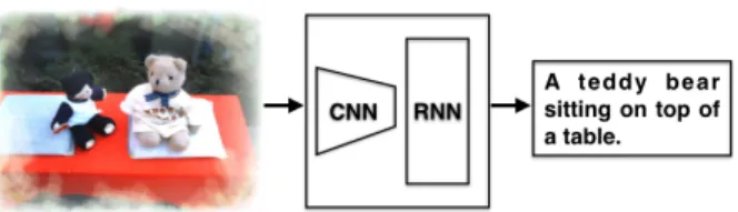
Figure 1: Image caption generation pipeline. The framework consists of a convulitional neural netwok (CNN) followed by a recurrent neural network (RNN). It generates an English sen-tence from an input image.

neural networks. By learning knowledge from age and caption pairs, the method can generate im-age captions that are usually semantically descrip-tive and grammatically correct.

Human beings usually describe a scene using natural languages which are concise and compact. However, machine vision systems describes the scene by taking an image which is a two dimension

arrays. From this perspective, Vinyalet al.(Vinyals

et al., ) models the image captioning problem as a language translation problem in their Neural Im-age Caption (NIC) generator system. The idea is mapping the image and captions to the same space and learning a mapping from the image to the

sen-tences. Donahue et al.(Donahue et al., ) proposed

a more general Long-term Recurrent Convolutional Network (LRCN) method. The LRCN method not only models the one-to-many (words) image cap-tioning, but also models many-to-one action genera-tion and many-to-many video descripgenera-tion. They also provides publicly available implementation based on Caffe framework (Jia et al., 2014), which further boosts the research on image captioning. This work is based on the LRCN method.

(2)

Although all the mappings are learned in an end-to-end framework, we believe the benefits of better understanding of the system by analyzing different components separately. Fig. 1 shows the pipeline. The model has three components. The first compo-nent is a CNN which is used to understand the con-tent of the image. Image understanding answers the typical questions in computer vision such as “What

are the objects?”, “Where are the objects?” and

“How are the objects interactive?”. For example, the CNN has to recognize the “teddy bear”, “table” and their relative locations in the image. The sec-ond component is a RNN which is used to generate a sentence given the visual feature. For example, the RNN has to generate a sequence of probabili-ties of words given two words “teddy bear, table”. The third component is used to generate a sentence by exploring the combination of the probabilities. This component is less studied in the reference paper (Donahue et al., ).

This project aims at understanding the impact of different components of the LRCN method (Don-ahue et al., ).We have following contributions:

• understand the LRCN method at the

implemen-tation level.

• analyze the influence of the CNN component

by replacing three CNN architectures (two from author’s and one from our implementa-tion).

• analyze the influence of the RNN component

by replacing two RNN architectures. (one from author’s and one from our implementation).

• analyze the influence of sentence generation

method by comparing two methods (one from author’s and one from our implementation).

2 Related work

Automatically describing the content of an image is a fundamental problem in artificial intelligence that connects computer vision and natural language pro-cessing. Earlier methods first generate annotations (i.e., nouns and adjectives) from images (Sermanet et al., 2013; Russakovsky et al., 2015), then gen-erate a sentence from the annotations (Gupta and

Mannem, ). Donahueet al.(Donahue et al., )

devel-oped a recurrent convolutional architecture suitable for large-scale visual learning, and demonstrated the

value of the models on three different tasks: video recognition, image description and video descrip-tion. In these models, long-term dependencies are incorporated into the network state updates and are end-to-end trainable. The limitation is the difficulty of understanding the intermediate result. The LRCN method is further developed to text generation from videos (Venugopalan et al., ).

Instead of one architecture for three tasks in

LRCN, Vinyals et al.(Vinyals et al., ) proposed a

neural image caption (NIC) model only for the im-age caption generation. Combining the GoogLeNet and single layer of LSTM, this model is trained to maximize the likelihood of the target descrip-tion sentence given the training images. The per-formance of the model is evaluated qualitatively and quantitatively. This method was ranked first in the MS COCO Captioning Challenge (2015) in which the result was judged by humans. Comparing LRCN with NIC, we find three differences that may indi-cate the performance differences. First, NIC uses GoogLeNet while LRCN uses VGGNet. Second, NIC inputs visual feature only into the first unit of LSTM while LRCN inputs the visual feature into every LSTM unit. Third, NIC has simpler RNN architecture (single layer LSTM) than LRCN (two factored LSTM layers). We verified that the math-ematical models of LRCN and NIC are exactly the same for image captioning. The performance dif-ference lies in the implementation and LRCN has to trade off between simplicity and generality, as it is designed for three different tasks.

Instead of end-to-end learning, Fanget al.(Fang

et al., ) presented a visual concepts based method. First, they used multiple instance learning to train visual detectors of words that commonly occur in captions such as nouns, verbs, and adjectives. Then, they trained a language model with a set of over 400,000 image descriptions to capture the

statis-tics of word usage. Finally, they re-ranked

cap-tion candidates using sentence-level features and a deep multi-modal similarity model. Their captions have equal or better quality 34% of the time than those written by human beings. The limitation of the method is that it has more human controlled param-eters which make the system less re-producible. We

believe the web applicationcaptionbot(Microsoft,

(3)

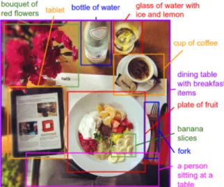
Figure 2:The visual-semantic alignment method can generate descriptions of image regions. Figure from (Karpathy and Fei-Fei, ).

Karpathyet al.(Karpathy and Fei-Fei, ) proposed

a visual-semantic alignment (VSA) method. The method generates descriptions of different regions of an image in the form of words or sentences (see Fig. 2). Technically, the method replaces the CNN with Region-based convolutional Networks (RCNN) so that the extracted visual features are aligned to

particular regions of the image. The experiment

shows that the generated descriptions significantly outperform retrieval baselines on both full images and on a new dataset of region-level annotations. This method generates more diverse and accurate descriptions than the whole image method such as LRCN and NIC. The limitation is that the method consists of two separate models. This method is fur-ther developed to dense captioning (Johnson et al., 2016) and image based question and answering sys-tem (Zhu et al., 2016).

3 Description of problem

Task In this project, we want to build a system that

can generate an English sentence that describes ob-jects, actions or events in an RGB image:

S =f(I) (1)

whereI is an RGB image andS is a sentence,f is

the function that we want to learn.

Corpus We use the MS COCO Caption (Chen et

al., 2015) as the corpus. The captions are

gath-ered from human beings using Amazon’s Mechani-cal Turk (AMT). We manually checked some exam-ples by side-by-side comparing the image and cor-responding sentences. We found the captions are very expressive and diverse. The COCO Caption is the largest image caption corpus at the time of writing. There are 413,915 captions for 82,783 im-ages in training, 202,520 captions for 40,504 imim-ages in validation and 379,249 captions for 40,775 im-ages in testing. Each image has at least 5 captions. The captions for training and validation are publicly available while the captions for testing is reserved by the authors. In the experiment, we use all the train-ing data in the traintrain-ing process and 1,000 randomly selected validation data in the testing process.

4 Method

For image caption generation, LRCN maximizes the probability of the description giving the image:

θ∗ = arg max θ

X

(I,S)

log p(S|I;θ) (2)

whereθare the parameters of the model,I is an

im-age, andS is a sample sentence. Let the length of

the sentence beN, the method applies the chain rule

to model the joint probability overS0,· · ·, SN:

log p(S|I) = N X

t=0

log p(St|I, S0,· · · , St−1) (3)

where the θ is dropped for convenience, St is the

word at stept.

The model has two parts. The first part is a CNN which maps the image to a fixed-length visual fea-ture. The visual feature is embedded to as the input

vto the RNN.

v=Wv(CNN(I)) (4)

whereWv is the visual feature embedding. The

vi-sual feature is fixed for each step of the RNN. In the RNN, each word is represented a one-hot

vectorSt of dimension equal to the size of the

dic-tionary. S0 and SN are for special start and stop

words. The word embedding parameter isWs:

(4)

In this way, the image and words are mapped to the same space. After the internal processing of the

RNN, the featuresv,xt and internal hidden

param-eterhtare decoded into a probability to predict the

word at current time:

pt+1 =LST M(v, xt, ht), t∈ {0· · ·N −1} (6)

Because a sentence with higher probability does not necessary mean this sentence is more accu-rate than other candidate sentences, post-processing

method such as Beam Search is used to generate

more sentences and pick top-K sentences.

4.1 Convolutional neural network

In this project, a convolutional neural network (CNN) maps an RGB image to a visual feature vec-tor. The CNN has three most-used layers: convolu-tion, pooling and fully-connected layers. Also,

Rec-tified Linear Units (ReLU) f(x) = max(0, x) is

used as the non-linear active function. The ReLU

is faster than the traditional f(x) = tanh(x) or

f(x) = (1 + e−x)−1. Dropout layer is used to prevent overfitting. The dropout sets the output of each hidden neuron to zero with a probability (i.e., 0.5). The “dropped out” neurons do not contribute to the forward pass and do not participate in back-propagation.

The AlexNet (Krizhevsky et al., 2012), VGGNet (Simonyan and Zisserman, 2014) and GoogLeNet (Szegedy et al., 2015) are three widely used deep convolutional neural network architecture.

They share the convolution → pooling →

fully-connection → loss function pipeline but with

dif-ferent shapes and connections of layers, especially the convolution layer. AlexNet is the first deep con-volutional neural network used in large scale image classification. VGGNet and GoogLeNet achieves the-start-of-the-art performance in ImageNet recog-nition challenge 2014 and 2015.

When the CNN combines the RNN, there are spe-cific considerations of convergence since both of them has millions parameters. For example, Vinyals

et al.(Vinyals et al., ) found that it is better to fix the parameters of the convolutional layer as the parame-ters trained from the ImageNet. As a result, only the non-convolution layer parameters in CNN and the RNN parameters are actually learned from caption examples.

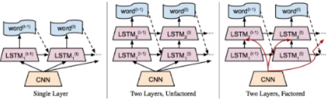
Figure 3: Three variations of the LRCN image captioning ar-chitecture. The most right two-layers factored LSTM is used in the method. Figure from (Donahue et al., ).

4.2 Recurrent neural network

To prevent the gradients vanishing problem, the long short-term memory (LSTM) method is used as the RNN component. A simplified LSTM updates for time steptgiven inputsxt,ht₋1, andct1 are:

it=σ(Wxixt+Whiht−1+bi) ft=σ(Wxfxt+Whfht₋₁+bf) ot=σ(Wxoxt+Whoht−1+bo) gt=φ(Wxcxt+Whcht−1+bc) ct=ftct−1+itgt ht=otφ(ct) (7) whereσ(x) = (1 +e−x)−1andφ(x) = 2σ(2x)−1.

In addition to a hidden unitht ∈ RN , the LSTM

includes an input gateit ∈ RN , forget gateft ∈

RN, output gate ot ∈ RN, input modulation gate

gt ∈ RN, and memory cell ct ∈ RN. These

ad-ditional cells enable the LSTM to learn extremely complex and long-term temporal dynamics. Addi-tional depth can be added to LSTMs by stacking them on top of each other. Fig. 3 shows three version of LSTMs. The two-layers factored LSTM achieves the best performance and is used in the method.

In this project, we proposed a simplified version of GRU in section 5.1 which also avoids the vanish-ing gradient problem and can be easily implemented in Caffe based on the current Caffe LSTM frame-work. We also provide the MATLAB program in the Appendices verifying our derivation of BPTT on the original GRU model.

4.3 Sentence generation

The output of LSTM is the probability of each word

in the vocabulary. Beam searchis used to generate

sentences. Beam search is a heuristic search algo-rithm that explores a graph by expanding the most promising node in a limited set. In addition to beam

(5)

search, we also use k-best search to generate sen-tences. It is very similar to the time synchronous

Viterbi search. The method iteratively selects thek

best sentences from all the candidate sentences up to

timet, and keeps only the resulting bestkof them.

5 Implementation

Preprocessing Because we want to keep the archi-tecture of the CNN, the input image are randomly

cropped to the size of224×224. As a result, only

part of the images are used in training at particular iteration. Because one image will be cropped mul-tiple times in the training, the CNN can probably see the whole image in the training (once for part of the image). However, the method only sees part of the image in the testing except the dense cropping is also used (our project does not use dense crop). For the sentences, the method first creates a vocabulary only from the training captions and removes lower frequency words (less than 5). Then, words are rep-resented by one-hot vectors.

5.1 Caffe architecture

Caffe (Jia et al., 2014) provides a modifiable frame-work for the state-of-the-art deep learning algo-rithms. It is implemented using C++ and also pro-vides Python and MATLAB interfaces. Caffe model (network) definitions are written as configuration

files using the Protocol Buffer Language1 so that

the net representation and implementation are sep-arated. The separation abstracts from memory un-derlying location in CPU or GPU so that switching between a CPU and GPU implementation is exactly by one function call. However, the separation makes the implementation less convenient as we will show in the next paragraph.

5.2 Simplify and implement GRU in Caffe

In Caffe, a layer is the fundamental unit of

com-putation. Ablob is a wrapper over the actual data

providing synchronization capability between CPU and GPU. We tried to implement the Gated Recur-rent Units (GRU) (Cho et al., 2014) in Caffe. The

GRU updates for time step t given inputs xt, st₋₁

1_{https://developers.google.com/} protocol-buffers/docs/proto are: z=σ(Uzxt+Wzst₋₁+bz) r=σ(Urxt+Wrst−1+br) h= tanh(Uhxt+Wh(st−1r) +bh) st= (1−z)h+zst−1 (8)

where z is the update gate, r is the reset gate. s

is used as both hidden states and cell states. With fewer parameters, GRU can reach a comparable per-formance to LSTM (Jozefowicz et al., ). To imple-ment GRU, we first wrote a MATLAB program to

check our BPTT2 gradient derivation. This is due

to the fact that automatic differentiation in Caffe is not supported at layer units level. Followed by our derivation, the calculated gradients only

devi-ate from the numerical gradients by around 10−5

relatively. However, implementing GRU in Caffe is not straight forward since Caffe is based on a complicated software architecture trying to provide convenience for assembling, not further developing. This is the bottleneck of GRU implementation. We have tried a number of implementations based on the original GRU (Equ. 8), with no good results. Finally we simplified GRU model inspired by the simplified SLTM in (Donahue et al., ). We omit the reset gate and add a transfer gate to make it easily fit into the current Caffe LSTM framework as:

z=σ(Uzxt+Wzst₋₁+bz) h= tanh(Uhxt+Whst−1+bh) ct= (1−z)h+zct−1 st=ct

(9)

Note that the omitted reset gate won’t bring back the vanishing gradient problem which we see in

tradi-tional RNN because we still have the update gatez

acting as a weight between the previous state and the

current processed input. The added transfer gate,c,

seems to be less useful, but it is actually very impor-tant for calculating the gradient in the framework. The parameter gradients in an RNN within a sin-gle step, t, depends not only on∂Lt/∂st, but also ∂Lt/∂st−i wherei = 1,2, ..., t. In Caffe,∂Lt/∂st

is calculated by outer layers automatically, while

∂Lt/∂st−ineed to be calculated by inside layer unit.

To hold and transfer these two parts of gradients to 2

(6)

CNNs layer #param memory B-4

AlexNet 8 60 0.9 0.253

VGGNet 16 138 11.6 0.294

GoogLeNet 22 12 5.8 0.211

Table 1: Quantitative comparison of CNNs. The number of parameter (#param) is in the unit of million, and the training memory is in the unit of Gb. In experiment, we found that the BLEU 4 performance is positively related to the number of pa-rameters.

the next time step, we use another intermediate

vari-able, which is the added transfer gate c. This is

just an engineering issue that might not be avoided while developing new models in Caffe. The theory is always clear and concise (see Appendices for the MATLAB program verifying our BPTT derivation to the original GRU).

5.3 Training method

The neural network is trained using the mini-patch stochastic gradient descent (SGD) method. The base learning rate is 0.01. The learning rate drops 50% in every 20,000 iterations. Because the number of training samples is much smaller than the number of parameters of the neural network, overfitting is our big concern. Besides the dropout layer, we fixed the parameters of the convolutional layers as suggested by (Vinyals et al., ). All the network are trained in a Linux machine with a Tesla K40c graphic card with 12Gb memory.

6 Results

6.1 Quantitative result

Evaluation metrics We use BLEU (Papineni et al., 2002) to measure the similarity of the captions generated by our method and human beings. BLEU is a popular machine translation metric that analyzes the co-occurrences of n-grams between the candi-date and reference sentences. The unigram scores (B-1) account for the adequacy of the translation, while longer n-gram scores (B-2, B-3, B-4) account for the fluency.

Different CNNs Table 1 compares the perfor-mance of three CNN architectures (the RNN part

Method B-1 B-2 B-3 B-4 AlexNet + LSTM 0.650 0.467 0.324 0.221 AlexNet + GRU 0.623 0.433 0.292 0.194 VGGNet + LSTM 0.588 0.406 0.264 0.168 VGGNet + GRU 0.583 0.393 0.256 0.168

Table 2: AlexNet, VGGNet with different RNN models. Our GRU model achieves comparable result with the LSTM model, but with less parameter and training time. The beam size is 1.

use LSTM). The VGGNet achieves the best perfor-mance (BLEU 4) and GoogLeNet has the lowest score. It is out of our expectation at first because GoogLeNet achieves the best performance in the Im-ageNet classification task. We discussed this phe-nomenon with our fellows students. One of them pointed out that despite its slightly weaker classi-fication performance, the VGGNet features outper-form those of GoogLeNet in multiple transfer learn-ing tasks (Karpathy, 2015). A downside of the VG-GNet is that it is more expensive to evaluate and it uses a lot more memory (11.6 Gb) and parameters (138 million). It takes more time to train VGGNet and GoogleNet than AlexNet (about 8 hours vs 4 hours).

Different RNNs Table 2 compares the perfor-mance of LSTM and GRU. The GRU model achieves comparable results with less parameters and training time.

Different sentence generation methods Table 3

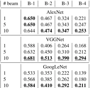
also analyze the impact of beam size in the Beam

Searchfor different CNN architectures. In general, larger beam size achieves higher BLEU score. This phenomenon is much more obvious in the VGGNet than other two CNNs. When the beam size is 1, AlexNet outperforms VGGNet. When the beam size is 10, the VGGNet outperforms AlexNet. The most probable reason is that AlexNet is good at detecting a single or few objects in an image while VGGNet is good at detecting multiple objects in the same im-age. When the beam size becomes larger, the VG-GNet based method can generate more accurate sen-tences.

(7)

# beam B-1 B-2 B-3 B-4 AlexNet 1 0.650 0.467 0.324 0.221 5 0.650 0.467 0.343 0.247 10 0.644 0.474 0.347 0.253 VGGNet 1 0.588 0.406 0.264 0.168 5 0.632 0.450 0.310 0.212 10 0.681 0.513 0.390 0.294 GoogLeNet 1 0.533 0.353 0.222 0.139 5 0.568 0.385 0.262 0.180 10 0.584 0.410 0.292 0.211 Table 3: AlexNet, VGGNet and GoogleNet with different beam sizes. Using AlexNet, the impact of the number of beam size is not significant. Using the VGG net, the impact is signif-icant. Using the GoogLeNet net, the impact is moderate. The best scores are highlighted.

Method B-1 B-2 B-3 B-4

LRCN 0.669 0.489 0.349 0.249

NIC N/A N/A N/A 0.277

VSA 0.584 0.410 0.292 0.211

This project 0.681 0.513 0.390 0.294

Table 4: Evaluation of image caption of different methods. LRCN is tested on the validation set (5,000 images). NIC is tested on the validation set (4,000 images). VSA is tested on the test set (40,775 images). This project is tested on the vali-dation set (1,000 images for B-1, B-2, B-3, and 100 images for B-4).

Comparison with other systems Table 4 com-pares BLEU scores of the results from LRCN, NIC, VSA and this project. The BLEU score of the re-sult of this project is comparable or better than those from other systems although our project is tested on less data set (1,000 images).

6.2 Qualitative result

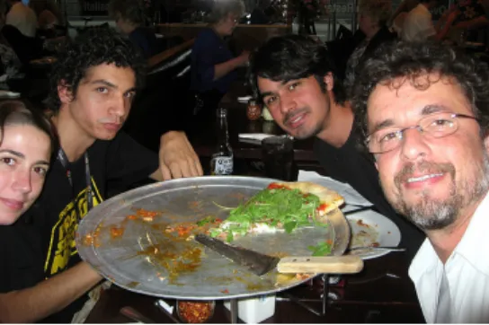
Taking Fig. 4 as an example, we analyze

the captions generated by AlexNet, VGGNet and GoogLeNet.

When beam size is 1, the captions are as follows,

• (AlexNet) A group of people sitting at a table

with a pizza.

• (VGGNet) A man and woman sitting at a table

with a pizza.

• (GoogLeNet) A group of people sitting at a

din-ner table.

• (AlexNet) A group of people sitting at a table.

• (VGGNet) A man and woman sitting at a table

with food.

din-ner table.

• (AlexNet) A group of people sitting at a table.

• (VGGNet) A man and woman sitting at a table.

din-ner table.

From the result listed above, we can see that when the beam size is fixed, VGGNet can generate cap-tions with more details. When the beam size creases, the captions become short and detailed in-formation disappears.

Although the sentence generated by our method has the highest probability, we don’t know if there are other sentences that can describe the image bet-ter. So we use 3-best search to explore the top 3 captions. For Fig. 4, the captions generated by GoogLeNet with beam size 5 using 3-best search are listed as follows,

• A group of people sitting at a dinner table.

• A group of people sitting around a dinner table.

• A group of people sitting at a dinner table with

plates of food.

The above captions are listed in probability de-scending order. We can see that the third sentence is actually the best one, although it does not have the highest probability. This is because when the sen-tence is long, it is more probable to make mistakes. So, sentences with high probability sometimes tend to be short, which may miss some detailed informa-tion. However, it does not mean that the sentence with the highest probability is bad. In most cases we observed, sentences with the highest probability are good enough to describe an image while long sentences often include redundant information and often make grammatical mistakes.

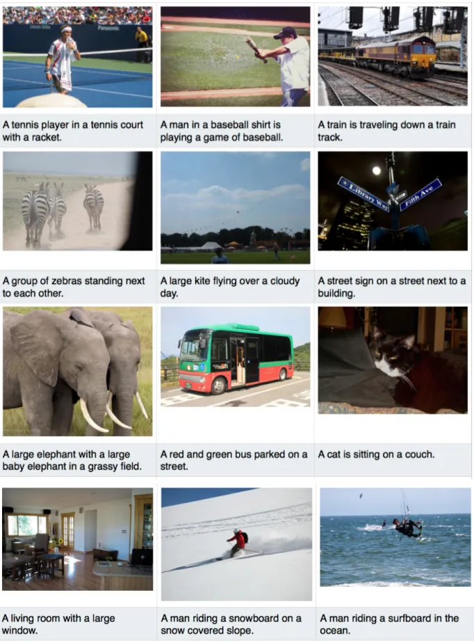
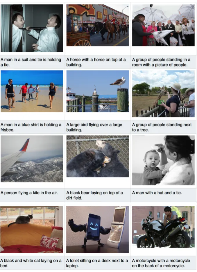
Fig. 5 shows the good examples of the sentences generated by this project. Most of them successfully describe the main objects and events in images. Fig. 6 shows failed examples of the system. The errors

(8)

Figure 4:Sample image for qualitative analysis.

are mainly from object mis-detections such as an airplane is mis-detected as a kite (row 3 column 1), cellphones are detected as laptop (row 4 column 2). The generated sentences are also has minor grammar error. For example, “A motorcycle with a motorcy-cle” (row 4 column 3) is hard to understand.

7 Lessons learned and future work

This project provides a valuable learning experience. First, the LRCN method has a sophisticated pipeline so that modifying part of the pipeline is complicated than we expected. We learned how to use one of the most popular deep learning frameworks Caffe through the project.

Second, mathematics and the knowledge of par-ticular software architecture are equally important for the success of the project. Although we imple-mented the MATLAB version of GRU very early before the deadline of the project, we spent a large amount of time on implementing the GRU layer in Caffe. The benefit is that we learned valuable first-hand experience on the developing level of Caffe in-stead of purely using existing layers in Caffe.

Third, working in a team, we could discuss and refine a lot of initial ideas. We could also antici-pate problems that could become critical of the cases we were working alone. Table 5 roughly shows the work division among team members.

8 Evaluation

• The project is successful. We have finished all

the goals before the deadline. The system can generate sentences that are semantically correct according to the image. We also proposed a simplified version of GRU that has less param-eters and achieves comparable result with the

Task Wenqiang Minchen Jianhui

CNN 100%

GRU 70% 30%

Beam Search 100%

Writing 40% 20% 40%

Table 5:Division of work. These only measure the implemen-tation and experimenting workload. All the analyses and dis-cussions are conducted by all of us.

LSTM method.

• The strength of the method is on its end-to-end

learning framework. The weakness is that it requires large number of human labeled data which is very expensive in practice. Also, the current method still has considerable errors in both object detection and sentence generation.

9 Conclusion and future work

We analyzed and modified an image captioning method LRCN. To understand the method deeply, we decomposed the method to CNN, RNN, and sen-tence generation. For each part, we modified or re-placed the component to see the influence on the final result. The modified method is evaluated on the COCO caption corpus. Experiment results show that: first the VGGNet outperforms the AlexNet and GoogLeNet in BLEU score measurement; second, the simplified GRU model achieves comparable re-sults with more complicated LSTM model; third, in-creasing the beam size increase the BLEU score in general but does not necessarily increase the quality of the description which is judged by humans.

Future work In the future, we would like to ex-plore methods to generate multiple sentences with different content. One possible way is to combine interesting region detection and image captioning. The VSA method (Karpathy and Fei-Fei, ) gives a direction of our future work. Taking Fig. 2 as an example, we hope the output will be a short para-graph: ”Jack has a wonderful breakfast in a Sunday morning. He is sitting at a table with a bouquet of red flowers. With his new iPad air on the left, he en-joys a plate of fruits and a cup of coffee.” The short paragraph naturally describes the image content in a story-telling fashion which is more attractive to the human beings.

(9)

(10)

(11)

References

[Chen et al.2015] Xinlei Chen, Hao Fang, Tsung-Yi Lin, Ramakrishna Vedantam, Saurabh Gupta, Piotr Dollar, and C Lawrence Zitnick. 2015. Microsoft coco

cap-tions: Data collection and evaluation server. arXiv

preprint arXiv:1504.00325.

[Cho et al.2014] Kyunghyun Cho, Bart Van Merrienboer, Caglar Gulcehre, Dzmitry Bahdanau, Fethi Bougares, Holger Schwenk, and Yoshua Bengio. 2014. Learn-ing phrase representations usLearn-ing rnn encoder-decoder

for statistical machine translation. arXiv preprint

arXiv:1406.1078.

[Donahue et al.] Jeffrey Donahue, Lisa Anne Hendricks, Sergio Guadarrama, Marcus Rohrbach, Subhashini Venugopalan, Kate Saenko, and Trevor Darrell. Long-term recurrent convolutional networks for visual recognition and description. InIEEE CVPR.

[Fang et al.] Hao Fang, Saurabh Gupta, Forrest Iandola, Rupesh K Srivastava, Li Deng, Piotr Dollar, Jianfeng Gao, Xiaodong He, Margaret Mitchell, John C Platt, et al. From captions to visual concepts and back. In

IEEE CVPR.

[Gupta and Mannem] Ankush Gupta and Prashanth Man-nem. From image annotation to image description. In

Neural information processing.

[Jia et al.2014] Yangqing Jia, Evan Shelhamer, Jeff Don-ahue, Sergey Karayev, Jonathan Long, Ross Girshick, Sergio Guadarrama, and Trevor Darrell. 2014. Caffe: Convolutional architecture for fast feature embedding. In Proceedings of the ACM International Conference on Multimedia, pages 675–678.

[Johnson et al.2016] Justin Johnson, Andrej Karpathy, and Li Fei-Fei. 2016. Densecap: Fully convolutional

localization networks for dense captioning. In IEEE

CVPR.

[Jozefowicz et al.] Rafal Jozefowicz, Wojciech Zaremba, and Ilya Sutskever. An empirical exploration of recur-rent network architectures. InICML.

[Karpathy and Fei-Fei] Andrej Karpathy and Li Fei-Fei. Deep visual-semantic alignments for generating image descriptions. InIEEE CVPR.

[Karpathy2015] Andrej Karpathy. 2015. Cs231n: Con-volutional neural networks for visual recognition.

http://cs231n.github.io/. [Online;

ac-cessed 11-April-2015].

[Krizhevsky et al.2012] Alex Krizhevsky, Ilya Sutskever, and Geoffrey E Hinton. 2012. Imagenet classification with deep convolutional neural networks. InAdvances in neural information processing systems.

[Microsoft] Microsoft. captionbot. https://www.

captionbot.ai/. [Online; accessed

22-April-2015].

[Papineni et al.2002] Kishore Papineni, Salim Roukos, Todd Ward, and Wei-Jing Zhu. 2002. Bleu: a method for automatic evaluation of machine translation. In

Proceedings of the 40th annual meeting on association for computational linguistics, pages 311–318. [Russakovsky et al.2015] Olga Russakovsky, Jia Deng,

Hao Su, Jonathan Krause, Sanjeev Satheesh, Sean Ma, Zhiheng Huang, Andrej Karpathy, Aditya Khosla, Michael Bernstein, et al. 2015. Imagenet large scale visual recognition challenge. IJCV, 115(3):211–252. [Sermanet et al.2013] Pierre Sermanet, David Eigen,

Xi-ang ZhXi-ang, Micha¨el Mathieu, Rob Fergus, and Yann LeCun. 2013. Overfeat: Integrated recognition, lo-calization and detection using convolutional networks.

arXiv preprint arXiv:1312.6229.

[Simonyan and Zisserman2014] Karen Simonyan and

Andrew Zisserman. 2014. Very deep convolutional

networks for large-scale image recognition. arXiv

preprint arXiv:1409.1556.

[Szegedy et al.2015] Christian Szegedy, Wei Liu,

Yangqing Jia, Pierre Sermanet, Scott Reed, Dragomir Anguelov, Dumitru Erhan, Vincent Vanhoucke, and

Andrew Rabinovich. 2015. Going deeper with

convolutions. InIEEE CVPR.

[Venugopalan et al.] Subhashini Venugopalan, Marcus

Rohrbach, Jeffrey Donahue, Raymond Mooney,

Trevor Darrell, and Kate Saenko. Sequence to

sequence-video to text. InIEEE ICCV.

[Vinyals et al.] Oriol Vinyals, Alexander Toshev, Samy Bengio, and Dumitru Erhan. Show and tell: A neu-ral image caption generator. InIEEE CVPR.

[Zhu et al.2016] Yuke Zhu, Oliver Groth, Michael

Bern-stein, and Li Fei-Fei. 2016. Visual7W: Grounded

(12)

Appendices

The MS COCO Caption corpus is in

http://mscoco.org/. Here is a list of code:

• GoogleNet with LSTM script.

• GRU MATLAB version.

• GRU layer Caffe implemenation.

• GRU unit layer Caffe implementation in C++

• GRU unit layer Caffe implementation in

CUDA C (running on GPU)

(13)

bottom: "inception_5b/pool_proj" top: "inception_5b/output" } layer { name: "pool5/7x7_s1" type: "Pooling" bottom: "inception_5b/output" top: "pool5/7x7_s1" pooling_param { pool: AVE kernel_size: 7 stride: 1 } } layer { name: "pool5/drop_7x7_s1" type: "Dropout" bottom: "pool5/7x7_s1" top: "pool5/7x7_s1" dropout_param { dropout_ratio: 0.4 } } layer { name: "loss3/classifier" type: "InnerProduct" bottom: "pool5/7x7_s1" top: "loss3/classifier" param { lr_mult: 1 decay_mult: 1 } param { lr_mult: 2 decay_mult: 0 } inner_product_param { num_output: 1000 weight_filler { type: "xavier" } bias_filler { type: "constant" value: 0 } } } # start LSTM layer {

(14)

num_output: 1000 weight_filler { type: "uniform" min: -0.08 max: 0.08 } bias_filler { type: "constant" value: 0 } } } layer { name: "lstm1" type: "LSTM" bottom: "embedded_input_sentence" bottom: "cont_sentence" top: "lstm1"

include { stage: "factored" } recurrent_param { num_output: 1000 weight_filler { type: "uniform" min: -0.08 max: 0.08 } bias_filler { type: "constant" value: 0 } } } layer { name: "lstm2" type: "LSTM" bottom: "lstm1" bottom: "cont_sentence" bottom: "loss3/classifier" top: "lstm2"

include { stage: "factored" } recurrent_param { num_output: 1000 weight_filler { type: "uniform" min: -0.08 max: 0.08 } bias_filler { type: "constant" value: 0

(15)

1% This program t e s t s t h e BPTT p r o c e s s we manually d e v e l o p e d f o r GRU. % We c a l c u l a t e t h e g r a d i e n t s o f GRU p a r a m e t e r s with c h a i n r u l e , and then 3% compare them t o t h e n u m e r i c a l g r a d i e n t s t o c h e c k whether our c h a i n r u l e

% d e r i v a t i o n i s c o r r e c t . 5

% Here , we p r o v i d e d 2 v e r s i o n s o f BPTT, b a c k w a r d d i r e c t ( ) and backward ( ) . 7% The f o r m e r one i s t h e d i r e c t i d e a t o c a l c u l a t e g r a d i e n t w i t h i n each s t e p

% and add them up (O( s e n t e n c e s i z e ˆ 2 ) time ) . The l a t t e r one i s o p t i m i z e d t o 9% c a l c u l a t e t h e c o n t r i b u t i o n o f each s t e p t o t h e o v e r a l l g r a d i e n t , which i s

% o n l y O( s e n t e n c e s i z e ) time . 11

% This i s v e r y h e l p f u l f o r p e o p l e who wants t o implement GRU i n C a f f e s i n c e 13% C a f f e didn ’ t s u p p o r t auto−d i f f e r e n t i a t i o n . This i s a l s o v e r y h e l p f u l f o r

% t h e p e o p l e who wants t o know t h e d e t a i l s about B a c k p r o p a g a t i o n Through 15% Time a l g o r i t h m i n t h e R e c c u r e n t N e u r a l Networks ( such a s GRU and LSTM)

% and a l s o g e t a s e n s e on how auto−d i f f e r e n t i a t i o n i s p o s s i b l e . 17

% NOTE: We didn ’ t i n v o l v e SGD t r a i n i n g h e r e . With SGD t r a i n i n g , t h i s 19% program would become a c o m p l e t e i m p l e m e n t a t i o n o f GRU which can be % t r a i n e d with s e q u e n c e data . However , s i n c e t h i s i s o n l y a CPU s e r i a l 21% Matlab v e r s i o n o f GRU, a p p l y i n g i t on l a r g e d a t a s e t s w i l l be d r a m a t i c a l l y

% s l o w . 23

% by Minchen Li , a t The U n i v e r s i t y o f B r i t i s h Columbia . 2016−04−21 25

. . . 27

% Forward p r o p a g a t e c a l c u l a t e s , y h a t , l o s s and i n t e r m e d i a t e v a r i a b l e s f o r each s t e p 29 f u n c t i o n [ s , y h a t , L , z , r , c ] = f o r w a r d ( x , y , . . . U z , U r , U c , W z , W r , W c , b z , b r , b c , V, b V , s 0 ) 31 % count s i z e s [ v o c a b u l a r y s i z e , s e n t e n c e s i z e ] = s i z e( x ) ; 33 i M e m s i z e = s i z e(V, 2 ) ; 35 % i n i t i a l i z e r e s u l t s s = z e r o s( iMem size , s e n t e n c e s i z e ) ; 37 y h a t = z e r o s( v o c a b u l a r y s i z e , s e n t e n c e s i z e ) ; L = z e r o s( s e n t e n c e s i z e , 1 ) ; 39 z = z e r o s( iMem size , s e n t e n c e s i z e ) ; r = z e r o s( iMem size , s e n t e n c e s i z e ) ; 41 c = z e r o s( iMem size , s e n t e n c e s i z e ) ; 43 % c a l c u l a t e r e s u l t f o r s t e p 1 s i n c e s 0 i s not i n s z ( : , 1 ) = s i g m o i d ( U z∗x ( : , 1 ) + W z∗s 0 + b z ) ; 45 r ( : , 1 ) = s i g m o i d ( U r∗x ( : , 1 ) + W r∗s 0 + b r ) ; c ( : , 1 ) = tanh( U c∗x ( : , 1 ) + W c∗( s 0 .∗r ( : , 1 ) ) + b c ) ; 47 s ( : , 1 ) = (1−z ( : , 1 ) ) .∗c ( : , 1 ) + z ( : , 1 ) .∗s 0 ; y h a t ( : , 1 ) = softmax (V∗s ( : , 1 ) + b V ) ; 49 L ( 1 ) =sum(−y ( : , 1 ) .∗l o g( y h a t ( : , 1 ) ) ) ; % c a l c u l a t e r e s u l t s f o r s t e p 2− s e n t e n c e s i z e s i m i l a r l y 51 f o r wordI = 2 : s e n t e n c e s i z e

z ( : , wordI ) = s i g m o i d ( U z∗x ( : , wordI ) + W z∗s ( : , wordI−1) + b z ) ;

53 r ( : , wordI ) = s i g m o i d ( U r∗x ( : , wordI ) + W r∗s ( : , wordI−1) + b r ) ;

c ( : , wordI ) = tanh( U c∗x ( : , wordI ) + W c∗( s ( : , wordI−1) .∗r ( : , wordI ) ) + b c ) ;

55 s ( : , wordI ) = (1−z ( : , wordI ) ) .∗c ( : , wordI ) + z ( : , wordI ) .∗s ( : , wordI−1) ;

y h a t ( : , wordI ) = so ftm ax (V∗s ( : , wordI ) + b V ) ;

57 L( wordI ) =sum(−y ( : , wordI ) .∗l o g( y h a t ( : , wordI ) ) ) ;

end 59 end 61% Backward p r o p a g a t e t o c a l c u l a t e g r a d i e n t u s i n g c h a i n r u l e % (O( s e n t e n c e s i z e ) time ) 63 f u n c t i o n [ dV , db V , dU z , dU r , dU c , dW z , dW r , dW c , db z , db r , db c , d s 0 ] = . . . backward ( x , y , U z , U r , U c , W z , W r , W c , b z , b r , b c , V, b V , s 0 ) 65 % f o r w a r d p r o p a g a t e t o g e t t h e i n t e r m e d i a t e and outp ut r e s u l t s [ s , y h a t , L , z , r , c ] = f o r w a r d ( x , y , U z , U r , U c , W z , W r , W c , . . . 67 b z , b r , b c , V, b V , s 0 ) ; % count s e n t e n c e s i z e 69 [ ˜ , s e n t e n c e s i z e ] = s i z e( x ) ; 71 % c a l c u l a t e g r a d i e n t u s i n g c h a i n r u l e d e l t a y = y h a t −y ; 73 db V = sum( d e l t a y , 2 ) ; 75 dV = z e r o s(s i z e(V) ) ; 1

(16)

f o r wordI = 1 : s e n t e n c e s i z e 77 dV = dV + d e l t a y ( : , wordI )∗s ( : , wordI ) ’ ; end 79 d s 0 = z e r o s(s i z e( s 0 ) ) ; 81 dU c = z e r o s(s i z e( U c ) ) ; dU r = z e r o s(s i z e( U r ) ) ; 83 dU z = z e r o s(s i z e( U z ) ) ; dW c = z e r o s(s i z e( W c ) ) ; 85 dW r = z e r o s(s i z e( W r ) ) ; dW z = z e r o s(s i z e( W z ) ) ; 87 d b z = z e r o s(s i z e( b z ) ) ; d b r = z e r o s(s i z e( b r ) ) ; 89 d b c = z e r o s(s i z e( b c ) ) ; d s s i n g l e = V’∗d e l t a y ;

91 % c a l c u l a t e t h e d e r i v a t i v e c o n t r i b u t i o n o f each s t e p and add them up

d s c u r = z e r o s(s i z e( d s s i n g l e , 1 ) , 1 ) ;

93 f o r wordJ = s e n t e n c e s i z e :−1 : 2

d s c u r = d s c u r + d s s i n g l e ( : , wordJ ) ;

95 d s c u r b k = d s c u r ;

97 dt anhInput = ( d s c u r .∗(1−z ( : , wordJ ) ) .∗(1−c ( : , wordJ ) .∗c ( : , wordJ ) ) ) ;

d b c = d b c + dtanhI nput ;

99 dU c = dU c + d tanhI npu t∗x ( : , wordJ ) ’ ; %c o u l d be a c c e l e r a t e d by a v o i d i n g add 0

dW c = dW c + d tanhInpu t∗( s ( : , wordJ−1) .∗r ( : , wordJ ) ) ’ ;

101 d s r = W c ’∗dt anhInput ; d s c u r = d s r .∗r ( : , wordJ ) ;

103 d s i g I n p u t r = d s r .∗s ( : , wordJ−1) .∗r ( : , wordJ ) .∗(1−r ( : , wordJ ) ) ;

d b r = d b r + d s i g I n p u t r ; 105 dU r = dU r + d s i g I n p u t r∗x ( : , wordJ ) ’ ; %c o u l d be a c c e l e r a t e d by a v o i d i n g add 0 dW r = dW r + d s i g I n p u t r∗s ( : , wordJ−1) ’ ; 107 d s c u r = d s c u r + W r ’∗d s i g I n p u t r ; 109 d s c u r = d s c u r + d s c u r b k .∗z ( : , wordJ ) ; dz = d s c u r b k .∗( s ( : , wordJ−1)−c ( : , wordJ ) ) ; 111 d s i g I n p u t z = dz .∗z ( : , wordJ ) .∗(1−z ( : , wordJ ) ) ; d b z = d b z + d s i g I n p u t z ; 113 dU z = dU z + d s i g I n p u t z∗x ( : , wordJ ) ’ ; %c o u l d be a c c e l e r a t e d by a v o i d i n g add 0 dW z = dW z + d s i g I n p u t z∗s ( : , wordJ−1) ’ ; 115 d s c u r = d s c u r + W z ’∗d s i g I n p u t z ; end 117 % s 1 119 d s c u r = d s c u r + d s s i n g l e ( : , 1 ) ; 121 dtanhInput = ( d s c u r .∗(1−z ( : , 1 ) ) .∗(1−c ( : , 1 ) .∗c ( : , 1 ) ) ) ;

d b c = d b c + dta nhI npu t ;

123 dU c = dU c + dtan hI nput∗x ( : , 1 ) ’ ; %c o u l d be a c c e l e r a t e d by a v o i d i n g add 0

dW c = dW c + dtanhInput∗( s 0 .∗r ( : , 1 ) ) ’ ; 125 d s r = W c ’∗dt anhInput ; d s 0 = d s 0 + d s r .∗r ( : , 1 ) ; 127 d s i g I n p u t r = d s r .∗s 0 .∗r ( : , 1 ) .∗(1−r ( : , 1 ) ) ; d b r = d b r + d s i g I n p u t r ; 129 dU r = dU r + d s i g I n p u t r∗x ( : , 1 ) ’ ; %c o u l d be a c c e l e r a t e d by a v o i d i n g add 0 dW r = dW r + d s i g I n p u t r∗s 0 ’ ; 131 d s 0 = d s 0 + W r ’∗d s i g I n p u t r ; 133 d s 0 = d s 0 + d s c u r .∗z ( : , 1 ) ; dz = d s c u r .∗( s 0−c ( : , 1 ) ) ; 135 d s i g I n p u t z = dz .∗z ( : , 1 ) .∗(1−z ( : , 1 ) ) ; d b z = d b z + d s i g I n p u t z ; 137 dU z = dU z + d s i g I n p u t z∗x ( : , 1 ) ’ ; %c o u l d be a c c e l e r a t e d by a v o i d i n g add 0 dW z = dW z + d s i g I n p u t z∗s 0 ’ ; 139 d s 0 = d s 0 + W z ’∗d s i g I n p u t z ; end testBPTT GRU.m 2

(17)

#include <string> #include <vector> #include "caffe/blob.hpp" #include "caffe/common.hpp" #include "caffe/filler.hpp" #include "caffe/layer.hpp" #include "caffe/sequence_layers.hpp" #include "caffe/util/math_functions.hpp" namespace caffe {

template <typename Dtype>

void GRULayer<Dtype>::RecurrentInputBlobNames(vector<string>* names) const { names->resize(2);

(*names)[0] = "s_0"; (*names)[1] = "c_0"; }

void GRULayer<Dtype>::RecurrentOutputBlobNames(vector<string>* names) const { names->resize(2);

(*names)[0] = "s_" + this->int_to_str(this->T_); (*names)[1] = "c_T";

}

void GRULayer<Dtype>::RecurrentInputShapes(vector<BlobShape>* shapes) const { const int num_output = this->layer_param_.recurrent_param().num_output(); const int num_blobs = 2;

shapes->resize(num_blobs);

for (int i = 0; i < num_blobs; ++i) { (*shapes)[i].Clear();

(*shapes)[i].add_dim(1); // a single timestep (*shapes)[i].add_dim(this->N_);

(*shapes)[i].add_dim(num_output); }

}

void GRULayer<Dtype>::OutputBlobNames(vector<string>* names) const { names->resize(1);

(*names)[0] = "s"; }

// modified from lstm_layer.cpp /* h -- > s

* c -- > c, omit the reset gate */

(18)

template <typename Dtype>

void GRULayer<Dtype>::FillUnrolledNet(NetParameter* net_param) const { const int num_output = this->layer_param_.recurrent_param().num_output(); CHECK_GT(num_output, 0) << "num_output must be positive";

const FillerParameter& weight_filler =

this->layer_param_.recurrent_param().weight_filler(); const FillerParameter& bias_filler =

this->layer_param_.recurrent_param().bias_filler();

// Add generic LayerParameter's (without bottoms/tops) of layer types we'll

// use to save redundant code.

LayerParameter hidden_param;

hidden_param.set_type("InnerProduct");

hidden_param.mutable_inner_product_param()->set_num_output(num_output * 2); hidden_param.mutable_inner_product_param()->set_bias_term(false);

hidden_param.mutable_inner_product_param()->set_axis(2); hidden_param.mutable_inner_product_param()->

mutable_weight_filler()->CopyFrom(weight_filler); LayerParameter biased_hidden_param(hidden_param);

biased_hidden_param.mutable_inner_product_param()->set_bias_term(true); biased_hidden_param.mutable_inner_product_param()->

mutable_bias_filler()->CopyFrom(bias_filler); LayerParameter sum_param;

sum_param.set_type("Eltwise");

sum_param.mutable_eltwise_param()->set_operation( EltwiseParameter_EltwiseOp_SUM);

LayerParameter scalar_param; scalar_param.set_type("Scalar");

scalar_param.mutable_scalar_param()->set_axis(0); LayerParameter slice_param;

slice_param.set_type("Slice");

slice_param.mutable_slice_param()->set_axis(0); LayerParameter split_param;

split_param.set_type("Split"); vector<BlobShape> input_shapes; RecurrentInputShapes(&input_shapes); CHECK_EQ(2, input_shapes.size()); net_param->add_input("c_0");

net_param->add_input_shape()->CopyFrom(input_shapes[0]); net_param->add_input("s_0");

net_param->add_input_shape()->CopyFrom(input_shapes[1]);

(19)

LayerParameter* cont_slice_param = net_param->add_layer(); cont_slice_param->CopyFrom(slice_param);

cont_slice_param->set_name("cont_slice"); cont_slice_param->add_bottom("cont");

cont_slice_param->mutable_slice_param()->set_axis(0);

// Add layer to transform all timesteps of x to the hidden state dimension.

// W_xc_x = W_xc * x + b_c

{

LayerParameter* x_transform_param = net_param->add_layer(); x_transform_param->CopyFrom(biased_hidden_param);

x_transform_param->set_name("x_transform"); x_transform_param->add_param()->set_name("W_xc"); x_transform_param->add_param()->set_name("b_c"); x_transform_param->add_bottom("x");

x_transform_param->add_top("W_xc_x"); }

if (this->static_input_) {

// Add layer to transform x_static to the gate dimension.

// W_xc_x_static = W_xc_static * x_static

LayerParameter* x_static_transform_param = net_param->add_layer(); x_static_transform_param->CopyFrom(hidden_param);

x_static_transform_param->mutable_inner_product_param()->set_axis(1); x_static_transform_param->set_name("W_xc_x_static");

x_static_transform_param->add_param()->set_name("W_xc_static"); x_static_transform_param->add_bottom("x_static");

x_static_transform_param->add_top("W_xc_x_static_preshape"); LayerParameter* reshape_param = net_param->add_layer(); reshape_param->set_type("Reshape");

BlobShape* new_shape =

reshape_param->mutable_reshape_param()->mutable_shape(); new_shape->add_dim(1); // One timestep.

// Should infer this->N as the dimension so we can reshape on batch size.

new_shape->add_dim(-1); new_shape->add_dim(

x_static_transform_param->inner_product_param().num_output()); reshape_param->add_bottom("W_xc_x_static_preshape");

reshape_param->add_top("W_xc_x_static"); }

LayerParameter* x_slice_param = net_param->add_layer(); x_slice_param->CopyFrom(slice_param);

x_slice_param->add_bottom("W_xc_x"); x_slice_param->set_name("W_xc_x_slice"); LayerParameter output_concat_layer; output_concat_layer.set_name("h_concat");

(20)

output_concat_layer.set_type("Concat"); output_concat_layer.add_top("s");

output_concat_layer.mutable_concat_param()->set_axis(0); for (int t = 1; t <= this->T_; ++t) {

string tm1s = this->int_to_str(t - 1); string ts = this->int_to_str(t);

cont_slice_param->add_top("cont_" + ts); x_slice_param->add_top("W_xc_x_" + ts);

// Add layers to flush the hidden state when beginning a new // sequence, as indicated by cont_t.

// h_conted_{t-1} := cont_t * h_{t-1} //

// Normally, cont_t is binary (i.e., 0 or 1), so: // h_conted_{t-1} := h_{t-1} if cont_t == 1 // 0 otherwise

{

LayerParameter* cont_h_param = net_param->add_layer(); cont_h_param->CopyFrom(scalar_param); cont_h_param->set_name("h_conted_" + tm1s); cont_h_param->add_bottom("s_" + tm1s); cont_h_param->add_bottom("cont_" + ts); cont_h_param->add_top("h_conted_" + tm1s); }

// Add layer to compute

// W_hc_h_{t-1} := W_hc * h_conted_{t-1} {

LayerParameter* w_param = net_param->add_layer(); w_param->CopyFrom(hidden_param); w_param->set_name("transform_" + ts); w_param->add_param()->set_name("W_hc"); w_param->add_bottom("h_conted_" + tm1s); w_param->add_top("W_hc_h_" + tm1s); w_param->mutable_inner_product_param()->set_axis(2); }

// Add the outputs of the linear transformations to compute the gate input. // gate_input_t := W_hc * h_conted_{t-1} + W_xc * x_t + b_c

// = W_hc_h_{t-1} + W_xc_x_t + b_c {

LayerParameter* input_sum_layer = net_param->add_layer(); input_sum_layer->CopyFrom(sum_param); input_sum_layer->set_name("gate_input_" + ts); input_sum_layer->add_bottom("W_hc_h_" + tm1s); input_sum_layer->add_bottom("W_xc_x_" + ts); if (this->static_input_) { input_sum_layer->add_bottom("W_xc_x_static");

(21)

}

input_sum_layer->add_top("gate_input_" + ts); }

// Add GRUUnit layer to compute the cell & hidden vectors c_t and s_t. {

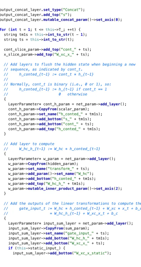
LayerParameter* gru_unit_param = net_param->add_layer(); gru_unit_param->set_type("GRUUnit"); gru_unit_param->add_bottom("c_" + tm1s); gru_unit_param->add_bottom("gate_input_" + ts); gru_unit_param->add_bottom("cont_" + ts); gru_unit_param->add_top("c_" + ts); gru_unit_param->add_top("s_" + ts); gru_unit_param->set_name("unit_" + ts); } output_concat_layer.add_bottom("s_" + ts); } // for (int t = 1; t <= this->T_; ++t) {

LayerParameter* c_T_copy_param = net_param->add_layer(); c_T_copy_param->CopyFrom(split_param); c_T_copy_param->add_bottom("c_" + this->int_to_str(this->T_)); c_T_copy_param->add_top("c_T"); } net_param->add_layer()->CopyFrom(output_concat_layer); } INSTANTIATE_CLASS(GRULayer); REGISTER_LAYER_CLASS(GRU); } // namespace caffe

(22)

#include <algorithm> #include <cmath> #include <vector> #include "caffe/layer.hpp" #include "caffe/sequence_layers.hpp" namespace caffe {

template <typename Dtype>

inline Dtype sigmoid(Dtype x) { return 1. / (1. + exp(-x)); }

inline Dtype tanh(Dtype x) { return 2. * sigmoid(2. * x) - 1.; }

void GRUUnitLayer<Dtype>::Reshape(const vector<Blob<Dtype>*>& bottom, const vector<Blob<Dtype>*>& top) {

const int num_instances = bottom[0]->shape(1); for (int i = 0; i < bottom.size(); ++i) { if (i == 2) { CHECK_EQ(2, bottom[i]->num_axes()); } else { CHECK_EQ(3, bottom[i]->num_axes()); } CHECK_EQ(1, bottom[i]->shape(0)); CHECK_EQ(num_instances, bottom[i]->shape(1)); } hidden_dim_ = bottom[0]->shape(2); CHECK_EQ(num_instances, bottom[1]->shape(1)); CHECK_EQ(2 * hidden_dim_, bottom[1]->shape(2)); top[0]->ReshapeLike(*bottom[0]);

top[1]->ReshapeLike(*bottom[0]); X_acts_.ReshapeLike(*bottom[1]); }

void GRUUnitLayer<Dtype>::Forward_cpu(const vector<Blob<Dtype>*>& bottom, const vector<Blob<Dtype>*>& top) {

const int num = bottom[0]->shape(1); const int x_dim = hidden_dim_ * 2;

const Dtype* C_prev = bottom[0]->cpu_data(); const Dtype* X = bottom[1]->cpu_data(); const Dtype* flush = bottom[2]->cpu_data(); Dtype* C = top[0]->mutable_cpu_data(); Dtype* S = top[1]->mutable_cpu_data(); for (int n = 0; n < num; ++n) {

for (int d = 0; d < hidden_dim_; ++d) {

const Dtype z = (*flush == 0) ? 0 : (*flush * sigmoid(X[d])); const Dtype h = tanh(X[hidden_dim_ + d]);

S[d] = C[d] = (1-z)*h + z*C_prev[d]; } C_prev += hidden_dim_; X += x_dim; C += hidden_dim_; S += hidden_dim_; ++flush; } }

(23)

void GRUUnitLayer<Dtype>::Backward_cpu(const vector<Blob<Dtype>*>& top, const vector<bool>& propagate_down, const vector<Blob<Dtype>*>& bottom) { CHECK(!propagate_down[2]) << "Cannot backpropagate to sequence indicators."; if (!propagate_down[0] && !propagate_down[1]) { return; }

const int num = bottom[0]->shape(1); const int x_dim = hidden_dim_ * 2;

const Dtype* C_prev = bottom[0]->cpu_data(); const Dtype* X = bottom[1]->cpu_data(); const Dtype* flush = bottom[2]->cpu_data(); const Dtype* C = top[0]->cpu_data(); const Dtype* S = top[1]->cpu_data(); const Dtype* C_diff = top[0]->cpu_diff(); const Dtype* S_diff = top[1]->cpu_diff();

Dtype* C_prev_diff = bottom[0]->mutable_cpu_diff(); Dtype* X_diff = bottom[1]->mutable_cpu_diff(); for (int n = 0; n < num; ++n) {

for (int d = 0; d < hidden_dim_; ++d) {

const Dtype z = (*flush == 0) ? 0 : (*flush * sigmoid(X[d])); const Dtype h = tanh(X[hidden_dim_ + d]);

Dtype* c_prev_diff = C_prev_diff + d; Dtype* z_diff = X_diff + d;

Dtype* h_diff = X_diff + hidden_dim_ + d; const Dtype c_term_diff = C_diff[d] + S_diff[d]; *c_prev_diff = c_term_diff * z;

*z_diff = c_term_diff * (C_prev[d] - h) * z * (1 - z); *h_diff = c_term_diff * (1 - z) * (1 - h*h); } C_prev += hidden_dim_; X += x_dim; C += hidden_dim_; S += hidden_dim_; C_diff += hidden_dim_; S_diff += hidden_dim_; X_diff += x_dim; C_prev_diff += hidden_dim_; ++flush; } } #ifdef CPU_ONLY STUB_GPU(GRUUnitLayer); #endif INSTANTIATE_CLASS(GRUUnitLayer); REGISTER_LAYER_CLASS(GRUUnit); } // namespace caffe

(24)

#include <algorithm> #include <cmath> #include <vector> #include "caffe/layer.hpp" #include "caffe/sequence_layers.hpp" namespace caffe {

__device__ Dtype sigmoid(const Dtype x) { return Dtype(1) / (Dtype(1) + exp(-x)); }

__device__ Dtype tanh(const Dtype x) {

return Dtype(2) * sigmoid(Dtype(2) * x) - Dtype(1); }

__global__ void GRUActsForward(const int nthreads, const int dim, const Dtype* X, Dtype* X_acts) { CUDA_KERNEL_LOOP(index, nthreads) {

const int x_dim = 2 * dim; const int d = index % x_dim; if (d < dim) {

X_acts[index] = sigmoid(X[index]); } else {

X_acts[index] = tanh(X[index]); }

} }

__global__ void GRUUnitForward(const int nthreads, const int dim, const Dtype* C_prev, const Dtype* X, const Dtype* flush, Dtype* C, Dtype* H) {

CUDA_KERNEL_LOOP(index, nthreads) { const int n = index / dim; const int d = index % dim;

const Dtype* X_offset = X + 2 * dim * n;

const Dtype z = (flush[n] == Dtype(0)) ? Dtype(0) : (flush[n] * X_offset[d]); const Dtype h = X_offset[dim + d];

const Dtype c_prev = C_prev[index];

H[index] = C[index] = z * c_prev + (Dtype(1)-z)*h; }

}

void GRUUnitLayer<Dtype>::Forward_gpu(const vector<Blob<Dtype>*>& bottom, const vector<Blob<Dtype>*>& top) {

const int count = top[1]->count();

const Dtype* C_prev = bottom[0]->gpu_data(); const Dtype* X = bottom[1]->gpu_data(); const Dtype* flush = bottom[2]->gpu_data(); Dtype* X_acts = X_acts_.mutable_gpu_data(); Dtype* C = top[0]->mutable_gpu_data(); Dtype* H = top[1]->mutable_gpu_data(); const int X_count = bottom[1]->count(); // NOLINT_NEXT_LINE(whitespace/operators)

GRUActsForward<Dtype><<<CAFFE_GET_BLOCKS(X_count), CAFFE_CUDA_NUM_THREADS>>>( X_count, hidden_dim_, X, X_acts);

CUDA_POST_KERNEL_CHECK;

// NOLINT_NEXT_LINE(whitespace/operators)

(25)

GRUUnitForward<Dtype><<<CAFFE_GET_BLOCKS(count), CAFFE_CUDA_NUM_THREADS>>>( count, hidden_dim_, C_prev, X_acts, flush, C, H);

CUDA_POST_KERNEL_CHECK; }

__global__ void GRUUnitBackward(const int nthreads, const int dim, const Dtype* C_prev, const Dtype* X, const Dtype* C, const Dtype* H, const Dtype* flush, const Dtype* C_diff, const Dtype* H_diff, Dtype* C_prev_diff, Dtype* X_diff) {

CUDA_KERNEL_LOOP(index, nthreads) { const int n = index / dim; const int d = index % dim;

const Dtype* X_offset = X + 2 * dim * n;

const Dtype z = (flush[n] == Dtype(0)) ? Dtype(0) : (flush[n] * X_offset[d]); const Dtype h = X_offset[dim + d];

const Dtype c_prev = C_prev[index]; const Dtype c = C[index];

Dtype* c_prev_diff = C_prev_diff + index; Dtype* X_diff_offset = X_diff + 2 * dim * n;

Dtype* z_diff = X_diff_offset + d;

Dtype* h_diff = X_diff_offset + dim + d;

const Dtype c_term_diff = C_diff[index] + H_diff[index]; *c_prev_diff = c_term_diff * z;

*z_diff = c_term_diff * (c_prev - h); *h_diff = c_term_diff * (Dtype(1) - z); }

}

__global__ void GRUActsBackward(const int nthreads, const int dim, const Dtype* X_acts, const Dtype* X_acts_diff, Dtype* X_diff) { CUDA_KERNEL_LOOP(index, nthreads) {

const int x_dim = 2 * dim; const int d = index % x_dim; const Dtype X_act = X_acts[index]; if (d < dim) {

X_diff[index] = X_acts_diff[index] * X_act * (Dtype(1) - X_act); } else {

X_diff[index] = X_acts_diff[index] * (Dtype(1) - X_act * X_act); }

} }

void GRUUnitLayer<Dtype>::Backward_gpu(const vector<Blob<Dtype>*>& top, const vector<bool>& propagate_down,

const vector<Blob<Dtype>*>& bottom) {

CHECK(!propagate_down[2]) << "Cannot backpropagate to sequence indicators."; if (!propagate_down[0] && !propagate_down[1]) { return; }

const int count = top[1]->count();

const Dtype* C_prev = bottom[0]->gpu_data(); const Dtype* X_acts = X_acts_.gpu_data(); const Dtype* flush = bottom[2]->gpu_data(); const Dtype* C = top[0]->gpu_data(); const Dtype* H = top[1]->gpu_data(); const Dtype* C_diff = top[0]->gpu_diff(); const Dtype* H_diff = top[1]->gpu_diff();

Dtype* C_prev_diff = bottom[0]->mutable_gpu_diff(); Dtype* X_acts_diff = X_acts_.mutable_gpu_diff();

GRUUnitBackward<Dtype> // NOLINT_NEXT_LINE(whitespace/operators)

<<<CAFFE_GET_BLOCKS(count), CAFFE_CUDA_NUM_THREADS>>>(count, hidden_dim_,

(26)

C_prev, X_acts, C, H, flush, C_diff, H_diff, C_prev_diff, X_acts_diff); CUDA_POST_KERNEL_CHECK;

const int X_count = bottom[1]->count(); Dtype* X_diff = bottom[1]->mutable_gpu_diff();

GRUActsBackward<Dtype> // NOLINT_NEXT_LINE(whitespace/operators)

<<<CAFFE_GET_BLOCKS(X_count), CAFFE_CUDA_NUM_THREADS>>>( X_count, hidden_dim_, X_acts, X_acts_diff, X_diff); CUDA_POST_KERNEL_CHECK;

}

INSTANTIATE_LAYER_GPU_FUNCS(GRUUnitLayer); } // namespace caffe

(27)

(28)