Balancing business and technical objectives for
supporting software product evolution
Muhammad Irfan Ullaha, Xueqi (David) Weib*, Barrie R. Naultc, Guenther Ruhea,da: Department of Computer Science, University of Calgary, T2N 1N4, Canada b: School of Management, Fudan University, P.R. China, 200433 c: Haskayne School of Business, University of Calgary, T2N 1N4, Canada
d: Department of Electrical and Computer Engineering, University of Calgary, T2N 1N4, Canada *Corresponding author. Tel: +86 21 2501 1242
E-mail addresses: [email protected] (M. Ullah), [email protected] (X. Wei), [email protected] (B. Nault) and [email protected] (G. Ruhe)
Abstract
Context: Successful software systems continuously evolve to accommodate feature requests of a diverse
customer-base. At some point during this evolution, the variety of customer needs and increased system complexity suggests the consideration of a software product line (SPL).
Aim: The goal of this research is to support the decision maker facing the enhancement of an evolving
software system (ESS) to determine the most appropriate product line design (out of a given set of candidate SPL portfolios) to minimize the technical risk and maximize the business value.
Method: The proposed method called OPTESS is aimed at finding an evolution plan for the ESS which
optimizes both the given technical and business objectives. Business analysis using a value-based pricing mechanism is applied to a set of initially proposed SPL portfolios (for enhancing the ESS) such that profit is maximized. Technical analysis is applied to the same initially proposed SPL portfolios to minimize the risk of failure of ESS due to implementation of new features. Business and technical analyses improve the performance of solutions for their respective objectives by modifying the feature sets of candidate SPL portfolios. OPTESS helps the decision maker to select a plan for enhancement of ESS by performing trade-off analysis on the economic and technical objectives.
Results: The method was initially evaluated by a case study for a set of 9 new candidate features to be
added to an open source text editing system called jEdit. OPTESS helped the decision maker to identify 3 non-dominated solutions considered to be of highest preference for decision-making when looking at both technical and economic criteria.
Keywords
Software engineering decision support, cost-benefit analysis, trade-off analysis, economic analysis, software product lines, software product evolution, open source systems
1
Introduction
Successful software systems continuously evolve to accommodate features requests from customers. This evolution of the system increases the complexity of the architecture thus increasing the cost of maintenance. On the other end, the customer-base of the software system is increasing owing to its success, attracting customers from diverse domains. At a certain point during the evolution of the system, the complexity of the architecture and the variations in customers’ needs triggers a SPL. A SPL is a set of software intensive systems that share a common, managed set of features satisfying the specific needs of a particular market segment or mission and that are developed from a common set of core assets in a prescribed way [1]. A number of real world software systems have evolved in this way. For example, Microsoft Windows operating system was initially launched as a single product. Due to its success, it was soon evolved into a SPL. One of the recent releases of this operating system, Windows Vista,
offers separate product variants for the home (Starter, Basic, Premium,) business (Business,
Enterprise) and power users (Ultimate) market segments where the term product variant refers to
an individual product in a SPL.
Despite several benefits of adopting a product line development approach (higher quality, productivity and return on investment) as reported in industrial case studies [1] [2], there is still resistance amongst practitioners towards its adoption. Several reasons have been reported for this resistance e.g., loss of product ownership, high upfront investment and lack of scientific evidence on economic benefits and risks of adopting a product line development approach [3]. Our previous works provided decision support to transition a single software product into a product line containing product variants addressing needs of specific customers’ segments. A suitable portfolio is selected from the candidate SPL portfolios for enhancing the ESS by analyzing the customers’ preferences for product features and the impact of the features on ESS’s structure [4] [5]. The decision support for evolving a single software product in [5] can be considered as a one dimensional approach since there is no consideration for the costs and economic benefits of the candidate SPL portfolios.
Most of the existing SPL development methods do not connect business and technical aspects for developing and evolving SPLs [6]. Our method provides a link between these two domains. The fundamental research question addressed by this paper is: Should a single software product facing feature requests for upcoming release be evolved into a software product line or not? Note that a single software product containing all the features for the upcoming release is always considered as one of the decision alternatives along with all the candidate SPL portfolios while evaluating the technical and business objectives.
In this paper, we present a method called OPTESS (Optimization of Technical and Business Objectives for Evolving Software Systems) which provides more comprehensive decision support for selecting an evolution plan for a single software product. In addition to the technical criterion, it also considers costs and expected revenues from candidate SPL portfolios for enhancing the ESS. The main content of the method is a trade-off analysis between technical risk and business value of candidate evolution plans for enhancing the ESS. For the scope of this paper, we define
technical risk as the probability that a feature implemented in an evolving software system’s
structure will cause failure of the system. The business value of a software product is calculated
by subtracting its estimated cost of development from the projected revenue. The specific research questions addressed in this paper are:
RQ 1: From a given set of candidate software product line portfolios for enhancing an evolving software system, which ones minimize the technical risk and maximize the business value?
To address the decision problem identified in RQ1, our proposed method brings together two different but equally important criteria. The first criterion is related to the technical aspects of evolving a single software product. For this purpose, we consider the impact of implementing new features in candidate SPL portfolios. The goal is to reduce the probability of failure when features are implemented in ESS’s structure. The technical aspect is addressed by the second research question.
RQ 2: How to estimate the risk of failure due to implementation of new features in the evolving software system’s architectural structure?
The second criterion is related to the economic benefits of enhancing the single software product to a SPL. For this purpose we calculate the costs and revenues of the single product and the candidate SPL portfolios. The goal is to identify SPL portfolios which maximize the economic benefits. Third research question addresses the economic aspect.
RQ 3: How to estimate the business value of a software product when considering both the revenue and the cost associated with the software product line design?
The specific technical contributions of this paper are:
(1) The decision support method OPTESS for trade-off analysis between technical risk and business value of candidate SPL portfolios.
(2) Customization of an existing technique to estimate risk of failure due to implementation of features in product variants being part of candidate SPL portfolios. (3) Application of an economic pricing and revenue generation method to estimate the
business value of each candidate SPL portfolio.
(4) A proof of concept of the method by application on an open source software system. The remainder of this paper is organized as follows: Section 2 presents the research work related to the solution approach. Section 3 presents background details of the techniques applied in the method OPTESS. Section 4 presents the method OPTESS. Section 5 presents an illustrative case study of the method on an open source software systems. Section 6 presents the applicability and limitation of the method. Section 7 presents the discussion with an outlook on future research direction.
2
Related Work
There are four main research areas that are related to the proposed method. These areas are decision support for software product evolution, risk estimation for implementing new features, product line cost models, and pricing and revenue generation for SPLs.
2.1
Decision support for software product evolution
The need for decision support arises when decisions have to be made in complex, uncertain and/or dynamic environments [7]. There are several works that address provision of decision support for various aspects of software systems development. Turban et al., suggest that decision support systems are most suitable for semi-structured and unstructured problems [8]. This is one of the key characteristics of wicked problems, i.e., they are difficult to formulate [9]. Planning releases for a single software product has been classified as a wicked problem [10]. Planning for a portfolio of products is even more challenging. This calls for greater efforts to develop methods and tools for supporting decision making process in product line engineering. Our previous work presented a decision support method COPE+ to address the fundamental research question presented in Section 1. COPE+, however, provides a one dimensional approach to address this problem by evaluating the alignment of candidate SPL portfolios with the architecture of the ESS. OPTESS adds a second dimension to this analysis by evaluating the economic benefits of the candidate SPL portfolios. In this section we present an overview of some of the existing methods that provide decision support for software product evolution.
Product Line Potential Analysis (PLPA) is a decision support approach (partly) addressing the research questions presented in Section 1 [11]. It is applied in a one day workshop for personnel of a business unit. The authors have developed a set of criteria which they suggest is important for answering this decision problem. These criteria are categorized as: main criteria (essential for
product line development and have to be fulfilled), inclusion criteria (indicates product line
already exists), supporting criteria (applied if a business unit has problems that product line
approach addresses) and exclusion criteria (to rule out factors that reduce economic advantage of
authors have prepared a questionnaire to get information on these criteria. The participants of the business unit are asked to fill out the questionnaire in the workshop. Their answers are then mapped to the criteria to address the decision problem. The results of this method are: yes (the
product line approach is suitable for these products and markets), no, or investigation required.
The focus of this method is to provide decision support at a higher level of abstraction without considering detailed attributes of the product portfolios. Additionally, it does not consider the cost and revenue of developing the product line.
Product Line Technical Probe (PLTP) assesses an organization’s readiness to adopt product line development approach [1]. It requires an organization-wide effort in which assessors gather information through structured interviews of key stakeholders. The results are a set of findings identifying the potential benefits, risks, as well as an assessment of the organization’s expertise regarding product line development approach. The risks and benefits are identified at the organizational level and not for an individual product or a product line.
Product Line Benefit and Risk Assessment method analyzes the benefits and risks for each of the technical domains associated with the product line [12]. Hence, instead of just saying yes or no to product line engineering, this method prioritizes technical domains for reuse potential. This
method has been modeled on the pattern of existing process maturity assessment methods. It does not evaluate the benefits and risks at the feature level.
Almost all systems development methods perform scoping at initial product definition stage to identify what (functionality) will be part of the system and what (functionality) will not be part of the system. This activity becomes even more important in SPL development since a product line contains multiple product variants. Most frameworks and methodologies for SPL development include scoping as a distinct activity. It is used to identify products within the product line (product portfolio scoping), features of these products as well as the features that will be developed for reuse (asset scoping) [13]. PULSE-Eco v2.0 is one such approach [13]. It relies on technical details such as economic benefit analysis to define products in the SPL. It does not, however, look into the ESS’s structure to analyze the impact of new features.
2.2
Risk estimation for implementing new features
The enhancement of the ESS to one of the candidate SPL solutions will require implementation of features in ESS’s structure. Each feature impacts one or more packages in the system structure. A package is a composition of classes in objected oriented design and refers to
an element of implementation as defined by Bass et al., in [14]. Packages represent a code-based way of considering the system structure. The purpose of risk estimation in this paper is to compare the candidate SPL solutions with respect to their risk of failure as a result of implementation of new features. There is an extensive body of knowledge on risk management for software systems. Boehm has identified top ten software risk items after investigating several large projects [15]. One of his findings is that as the size of the requirement increases, the probability of failure also increases.
Two types of approaches have been proposed in literature to estimate the probability that a change (due to a bug fix or new feature implementation) in a software system will cause its failure. The techniques in the first approach use product measures such as size of the file, degree of nesting, code complexity (such as McCabe’s cyclomatic complexity) to predict the probability of failure. The techniques in the second approach for modeling fault rates use data from the change and defect history of the program. Both types of approaches are applicable for the purpose of our method; however, we are more interested in estimating the probability of failure using the product measures rather than historical data.
Therefore, we have selected and adapted a technique by Mockus and Weiss [16] to estimate the probability of failure of the ESS. They have proposed a risk estimation model that estimates the probability of failure by using the “change measures” for the feature being implemented. These change measures capture information such as the number of packages modified for implementing the feature, the number of lines of code added or deleted, the duration for implementing the feature and experience of the developer. This model estimates the risk for one feature implementation in isolation. However, in our case, each product variant (in a given SPL portfolio) is typically developed by implementing more than one feature. Therefore, we have customized their model to estimate risk.
2.3
Product line cost models
Boehm defines economics as the, “study of how people make decisions in resource-limited situations” [17]. The investment in establishing a product line enables the development organization to improve quality, capture diverse markets, eventually increasing its revenues and profits as reported in many case studies [1] [2]. Due to large upfront cost and risk of failure, there is always a hesitation in industry to adopt product line development [3] [18]. Method OPTESS tries to address this concern by providing technical and economic benefit analysis for the candidate SPL solutions.
There is a large body of knowledge on cost estimation of software products [17]. We present an overview of the most popular cost estimation models for SPL development.
The Constructive Product Line Investment Model (COPLIMO) is based on the COCOMO II model [19]. COPLIMO determines the cost of a SPL in two components. The first component reflects the cost of initial development of the SPL architecture and the second component reflects the post-development extensions. The second cost component incorporates the reuse of previously developed components by the products developed later in the development life cycle. qCOPLIMO extends the COPLIMO model by evaluating the additional benefits in product line development through higher quality [20].
Structured Intuitive Model for Product Line Economics (SIMPLE) provides a high level framework for estimating the cost of developing a SPL [21]. It provides four cost functions that can be combined in a number of ways to estimate the cost of establishing a SPL. Boeckle et al., present seven scenarios that cover several possibilities of evolving and instantiating a SPL. As opposed to COPLIMO, SIMPLE does not look into the costs and revenues from future extensions of the product line. Since we are only considering the cost of evolving the ESS into a SPL in one release, we selected SIMPLE to estimate the cost of the SPL in our method.
Application of SIMPLE requires effort estimates for the features. Effort estimation methods for software systems fall into three main categories: expert judgment, estimation by analogy, and algorithmic cost estimation [22]. Expert judgment relies on the experience of experts. The accuracy of expert based prediction is low. Algorithmic estimation involves the application of mathematical models such as in COPLIMO [19]. The idea of analogy-based estimation is to determine the effort of the target feature (or project) as a function of the known effort from similar historical features (or projects). Compared with the other two categories, estimation by analogy performed best in 60% of the published case studies [23]. Existing analogy-based effort estimation methods have several limitations. For example, the CATREG method proposed by Angelis et al., can only work with data sets containing categorical (or qualitative) attributes [24]. Many of the existing analogy-based effort estimation techniques can only work data sets without any missing values [25]. Method AQUA proposed by Li and Ruhe in [25] supports multiple data types by defining similarity measures for these data types. It is also able to tolerate missing values in the data set. AQUA has performed better than other analogy-based effort estimation techniques
using publicly available data sets. We have selected AQUA to implement cost functions of SIMPLE.
2.4
Pricing and revenue generation for SPLs
Pricing and revenue generation for SPLs have been broadly explored in the economic and marketing literatures. The major purpose of the SPL design by an organization is to meet the requirements of customers in different market segments to maximize its profit. Pricing of a SPL is normally determined by the value-based pricing mechanism, which is to set prices for different product variants according to customers’ valuations [26].
Moorthy [27] proposed a customer self-selection model to evaluate the product line design strategies of a monopolist. He argued that customers should be able to choose their preferred products freely and the optimal product line design strategies should address this in order to maximize the overall profits of the product line. In order to make customer self-selection work for SPL design, the individual rationality (IR) and incentive compatibility (IC) constraints are normally imposed on pricing of a SPL [28]. The IR constraint ensures that a consumer gets non-negative surplus from purchasing their chosen product variant and the IC constraint indicates that the consumer prefers product variant that maximizes her surplus.
Product variants in a SPL can be either horizontally or vertically differentiated. For vertical differentiation, a product variant includes all the features of another product variant and more, while for horizontal differentiation; different product variants include some special features of their own although they usually share some common features. Wei and Nault [29] proposed analytical models to develop product line design strategies under both situations when a monopolist chooses to offer different products to meet the special requirements of different groups of customers to maximize its overall profit. In our method, we follow Wei and Nault [29] to calculate revenues generated from a product line in order to estimate its business value.
3
Background
SPL development aims at maximizing profit. This includes two parts: (i) cost of establishing a SPL and (ii) revenue generated from the product line. To estimate costs of establishing a SPL, we adopt the SIMPLE model [21]. To maximize revenues from a SPL, we follow pricing strategies of information goods developed in information systems economics based on economics and marketing research and adjust them to the purposes of this research. To estimate the risk of failure by implementing new features in the ESS, we customize an existing risk estimation method. In the following subsections, we present an overview of these techniques.
3.1
SIMPLE
SIMPLE proposed by Boeckle et al., provides a framework to estimate the cost of developing a SPL [21]. SIMPLE is selected to estimate the costs of candidate SPL portfolios for the reasons discussed in Section 2.3. The model has four cost functions. Each of the four cost functions of SIMPLE represents a separate idea and can be implemented through a variety of approaches. Below we provide an overview of the four cost functions that can be combined in a number of scenarios for initiating or evolving a product line:
(1) Cunique(): This function, given the relevant parameters, returns the cost to develop unique software that is not based on a product line platform. Usually, this will be a small portion of the product but in the extreme it could be a
complete product. We apply the method AQUA [25] to estimate the effort (in person months) for implementing each unique feature.
(2) Ccab(): This function returns the cost to develop the shared features for a SPL portfolio. The shared features cost more than unique features because of the variability required to support multiple product variants. We include this additional effort by considering the packages in ESS’s structure impacted by the shared features and correspondingly adjust the effort estimates suggested by AQUA [25].
(3) Creuse(): This function returns the cost to reuse the shared features in multiple product variants. It includes the cost of tailoring it (by applying appropriate variability mechanisms) for use in the intended product variant and performing the extra integration tests. We follow the recommendations by experts [37] to estimate the cost of reusing shared features across multiple product variants in a SPL.
(4) Corg(): This function returns the cost for an organization to adopt a product line development approach for its products. Such costs can include reorganization, process improvement, training and other organizational remedies as necessary.
With these functions, however implemented, it can be observed that the cost of developing the
i-th SPL portfolio can be expressed as:
Cost(i) = Cunique(i) + Ccab(i) + Creuse(i) + Corg(i) (1)
These cost functions form the basis for a number of different scenarios of instituting or evolving a SPL [21]. One such scenario will be considered in details in Section 5.3.2.
3.2
Pricing and Revenue Generation Applied to SPL
After a SPL portfolio has been designed, appropriate pricing strategies are implemented to maximize its revenue. In this paper, we assume a customer self-selection market [27] where a customer selects any product variant to maximize surplus which equals to the value the customer gets from the product variant minus price of this product variant. The customer self-selection assumption has been widely adopted to explore pricing of product variants in SPL portfolios [28] [29].
In our method, we follow Wei and Nault [29] to calculate the overall revenue generated from a SPL to lay an economic basis for the estimation of the business value of the SPL design. Revenue generated from the SPL is the sum of revenues from all the market segments. Thus the total revenue generated from a SPL portfolio depends on two variables: price of each product variant and number of customers who purchase the specified product variant. To specify the revenue generation of a SPL portfolio, we define the following variables:
Definition 1 (Revenue R(p(i,j))): The revenue generated from the j-th product variant in the
i-th SPL portfolio. In a self-selection market, i-the revenue equals to i-the uniform price times i-the total number of customers who adopt this product variant.
Definition 2 (Price of each product variant P(p(i,j))): The price of the j-th product variant in
the i-th SPL portfolio. In a self-selection market, the price of the product variant p(i,j) is the same
for all the customers.
Definition 3 (Customer’s valuation Vk(p(i,j))): Customer k’s valuation for the product variant p(i,j).. In our model, the customer’s valuation of a product variant is determined through the feature voting scores.
In order to make customer self-selection work, two classical constraints must be satisfied: the IR constraint and the IC constraint. As discussed earlier, the IR constraint indicates that a customer always gets non-negative consumer surplus from purchasing a certain product variant. If the price for a certain product variant p(i,j) is higher than the value the customer can get from it, the customer would choose not to buy. Thus the IR constraint can be expressed as:
Vk(p(i,j)) - P(p(i,j)) 0, for all p(i,j) (2)
In order to maximize revenue, some consumers with low valuation may not purchase any product variant if prices of all product variants are set higher than their valuation, in other words, not all customers are necessarily to be served with a product variant.
The IC constraint indicates that when there are many product variants for the customer to choose from, the one chosen maximizes consumer surplus. It means the customer k gets most consumer surplus from purchasing product variant p(i,j) than any other product variant p(i,l). The IC constraint can be expressed as:
Vk(p(i,j)) - P(p(i,j)) Vk(p(i,l)) - P(p(i,l)), for all p(i,j) and p(i,l) (3) The IC and IR constraints determine the price relationship of different product variants in a SPL portfolio. More details will be discussed in the cost-benefit analysis in Section 4.2.2.
Definition 4 (Q(p(i,j))): The quantity of a product variant p(i,j). For a specified product
variant p(i,j), the total number of customers depends on the price of the product variant and the valuation of each customer.
The total revenue generated from the ith SPL portfolio is the sum of revenues generated from
each product variant. Thus, we express the total revenue as:
R(i) ∑j( P(p(i,j)) * Q(p(i,j))) (4)
The combination of revenue generated from a SPL portfolio and relevant costs associated with the product line development determines the business value of that portfolio.
3.3
Estimating Risk of Software Change
Mockus and Weiss’s have proposed a model for estimating risk of implementing a maintenance request in a software system [16]. They consider implementation of each maintenance request (MR) in isolation. For the purpose of this work, we assume that multiple MRs (or product features) are implemented sequentially to develop a product variant in any given SPL portfolio. Correspondingly, we have replaced the diffusion (DF) metric of originally
proposed model by Mockus and Weisss with another metric, which we call as adjusted diffusion
Definition 5 (Maintenance request): For this work we will assume that an MR is the request to
implement one new feature in the ESS.
Mockus and Weiss’s model uses the following five metrics to estimate the probability that a change implemented as a result of an MR will cause failure in the software system:
Definition 6 (Diffusion): Diffusion (DF) is the number of distinct subsystems modified in the
ESS’s structure to implement the change.
Definition 7 (Delta): Delta is an atomic change to the source code recorded by a version
control system. Each MR may require changes to several source code files. A file may be changed several times. Each change to a file is called a delta. The model uses the total number of deltas (ND) for an MR to predict probability of failure.
Definition 8 (Interval): Interval (INT) is the time between the last and first delta.
Definition 9 (Experience): Average experience (EXPR) of the developer implementing the
change.
Definition 10 (Lines of Code Added): Lines of code added (LA) represent the size of the
change to implement the MR.
We have defined a new metric, adjusted diffusion (ADF) which replaces the diffusion (DF)
metric.
Definition 11 (Adjusted Diffusion): Adjusted diffusion (ADF) is the number of distinct
subsystems modified in the ESS to implement all the MRs (features) for a product variant in a given SPL portfolio.
The above mentioned criteria are combined in the following model to estimate the probability of failure (P) as shown in Equation 5. αi represent the estimated coefficients for the five parameters.
)
1
LA
(
EXP
INT
ND
ADF
e
1
)
1
LA
(
EXPR
INT
ND
ADF
e
P
5 4 3 2 1 5 4 3 2 1+
α
α
α
α
α
+
+
α
α
α
α
α
=
• + • + • + • + • • + • + • + • + • (5)4
Method OPTESS
4.1Overview
The idea of offering decision support arises when decisions have to be made in complex, uncertain and/or dynamic environments. In software development and evolution, many decisions have to be made concerning processes, products, tools, methods and techniques. From a decision-making perspective, all these questions are confronted by different objectives, constraints, and a huge number of variables under dynamically changing requirements. Very often, this is combined with incomplete, fuzzy or inconsistent information about all the involved artifacts, as well as with difficulties regarding the decision space and environment [7].
The method OPTESS has three modules as shown in Figure 1. The method requires that segments of customers and their corresponding products be available as input. This input is generated by our previous works [4] [30]. Another input is related to the impact of new features on ESS’s architectural structure. Feature impact analysis techniques and tools are available to generate this information. Interested reader is referred to [5] for a discussion on such techniques. Figure 1 shows the workflow of COPE+ illustrated as a UML activity diagram. Elements with
identifiers Ai are the activities which take one or more input artifacts (data) identified as Oi. An
activity manipulates input artifacts to produce at least one output artifact. These activities are arranged in three modules. The human decision maker is involved at various stages of the decision support to analyze and update the data and results. A brief overview of the modules is presented below.
Figure 1 Workflow of OPTESS illustrated as a UML Activity diagram
Starting with an initial set of SPL portfolios, the first module of OPTESS called Business-adjustments modifies the feature sets (by adding or removing features) of the product variants to
increase the business value of the portfolios. The output of module 1 is a set of business-adjusted SPL portfolios.
The second module called Structural-adjustments modifies the feature sets of the product
portfolios (by adding or removing features) using the information on how these features impact the ESS’s structure. A human decision maker is involved in this process to finalize the changes to the feature sets. Selecting features in product variants that impact a cohesive set of subsystems in
ESS’s structure will reduce the probability of failure of the system when these features are implemented.
The first two modules generate SPL portfolios that are optimized either on the business objective or the technical objective. The purpose of module 3 called Trade-off-analysis is to allow
the decision maker to perform trade-off between technical and business objectives. This module takes the business-adjusted portfolios (from module 1) and structural-adjusted portfolios (from module 2) and combines them in a set of candidate SPL portfolios. A customized risk estimation technique is applied to determine the risk of implementing new features for all candidate product portfolios. A product line cost estimation model is applied to determine the cost of developing the candidate SPL portfolios. Our previous work from software versioning is applied to determine the pricing structure, revenues and business value for each candidate SPL portfolio. A trade-off analysis is performed between the technical risk and business value of the candidate product portfolios to identify the non-dominated solutions. The decision maker analyzes these suggested solutions and selects a final solution.
4.2
Module 1: Business-adjusted solutions
4.2.1 Valuation-based adjustmentAfter the initial SPL solutions are generated from the clustering method [30], we explore the possible adjustment of the SPL solutions to find out the profit-maximizing portfolios.
In the valuation-based adjustment, whether a feature should be included in certain product variant of a SPL is adjusted according to the customer’s valuation. In our model, the customer’s valuation of certain features is measured by their initial voting scores. The adjustment is done according to the following three rules:
Rule 1: If customers and features can be determined by the clustering method, then features
included in each product variant correspond to the clustering results.
Rule 2: If features associated with certain customer segment are not the result of the application
of the clustering method, then features with a majority of the customer segment whose initial votes are above a pre-defined threshold are included in the product variant.
Rule 3: Product variants which cannot satisfy the IC and IR conditions are removed from the SPL.
In order to maximize revenue from the SPL portfolio, some product variants may be combined together to better satisfy the IC and IR conditions for optimal software pricing. In our model, we measure all possible combinations of clusters of customers to generate various possible SPL portfolios. In Section 5, we illustrate this process through an example case study.
4.2.2 Analyze profit-maximizing portfolios
For each possible SPL portfolio, we apply the IR and IC conditions to set the optimal prices for each product variant. The revenue generated is a sum of revenues from all product variants in a product line.
Because the prices are set according to customers’ valuation of features and the costs are measured in person months, we introduce a conversion factor β to convert cost into dollar value.
Definition 12 (Conversion factor β): The conversion factor β indicates the conversion rate
between person-months and dollars.
We assume there is no variable cost associated for creation and distribution of any additional copy of a product variant. The profit of a SPL portfolio is defined as:
Definition 13 (Estimated profit of a portfolio): Profit from the i-th SPL portfolio is measured by a
subtraction of total revenue generated from the product line by cost associated with creation of the SPL.
The estimated profit of the i-th SPL portfolio is measured as:
Profit(i) R(i) – β * Cost(i) (6)
4.3
Module 2: Structural-adjusted solutions
The product portfolios given as input to the method OPTESS are generated using customers’ preference structure on product features. Each one of the new features in these product portfolios impacts a subset of packages in the ESS’s structure. To analyze the impact of features on ESS’s structure, we identify sub-systems in ESS’s structure. A sub-system is a cohesive group of packages that implement a group of features. A human decision maker adds or removes features from the product variants of initially proposed SPL portfolios according to the following rules:
Rule 1: If all the features implemented in a subsystem in ESS’s structure are present in a product
variant then none of them is removed from the product variant.
Rule 2: If more than or equal to θadj of the features implemented in a subsystem in ESS’s
structure are present in a product variant then remaining features corresponding to the same subsystem are included in the feature set of that product variant. The value of the parameter θadj can vary between 0 to 100%.
Rule 3: If less than θadj of the features implemented in a subsystem in ESS’s structure are present
in a product variant then they are removed from the feature set of that product variant.
The value of the parameter θadj is set by the human decision maker keeping in view the time and resource availability for the release. For a resource limited scenario, θadj can be set very high which will reduce the impact of features on ESS’s structure, consequently reducing the effort required to complete the release. The structural adjustments decrease the diffusion of the features of product variants (in any given SPL portfolio) consequently reducing the risk of failure. Note that the fifty percent (representing half of the features for a given subsystem) threshold value for adding or removing features is a parameter and can be changed. A human expert finalizes the structural adjustments by considering other constraints, such as pre-assignment and coupling. This activity is illustrated in Section 5.2.
4.4
Module 3: Trade-off analysis
The business-adjusted solutions from module 1 and the structural-adjusted solutions from module 2 are combined to form a set of candidate SPL portfolios. Module 3 allows the decision maker to perform trade-off analysis for candidate SPL portfolios.
4.4.1 Technical risk estimation
The technical risk of developing a product variant in any given SPL portfolio is calculated using the model presented in Equation (5). In Section 5.3.1, we present an example to illustrate the computation of the technical risk for implementing new features in an open source software system. This activity of module 3 addresses RQ2.
4.4.2 Cost estimation
To estimate the cost of developing a candidate SPL portfolio, we apply Equation (1) of the SIMPLE model. Out of the four cost functions of SIMPLE, we are not including the
organizational and process related costs, calculated by the function Corg(). Assuming that Corg(), is constant for all the candidate SPL portfolios, the trade-off analysis will not be impacted significantly by this assumption. In Section 5.3.2, we illustrate the cost estimation by evaluating the cost functions of SIMPLE for the example software system.
4.4.3 Price estimation
Prices of each product variants are set to maximize total revenue that can possibly be generated from a SPL. In order to segment customers effectively in a self-selection market, we impose the IR and IC constraints in Equations (2) and (3).
In the price estimation process, we start to set price for the product variant with least number of features. With the IR constraint, the initial price of the product variant is set to maximize revenue of this market segment only. When more market segments are included, the IC constraint is imposed to make sure customers can self-select their preferred product variants.
With the purpose to maximize total revenue of a SPL, price of each product variant may be higher than valuation of some customers in the market. That means not all customers are necessarily served and the market may not be fully covered.
4.4.4 Business value estimation
Business value is estimated through balancing total revenue generated from the SPL and total costs that are associated with the SPL. The total revenue is calculated according to Equation (4) and the total costs are measured in Equation (1). Thus the business value of a SPL, which is equivalent to the overall profit from the SPL, is estimated using Equation (6). This activity of module 2 addresses RQ3.
4.4.5 Identification of non-dominated solutions
In the final activity of module 3, the non-dominated SPL portfolios are identified using the business value and technical risk estimates. Given a bi-objective optimization problem F(x), x* is
said to be a Pareto-optimal solution (or a non-dominated solution) of the bi-objective problem if x*∈X and there does not exist any other solution x which dominates x* when the values of both
the objectives are considered together.
The bi-objective optimization problems typically present a set of compromised optimal values. The set of solutions resulting from these optimal values are called as Pareto-optimal solutions if
there are no other solutions that are superior to them when the two objectives are considered. These set of solutions are referred to as non-dominated. For this work the non-dominated solutions are the SPL portfolios which perform better than all other candidate portfolios when both the business value and technical risk estimates are considered together. Several Pareto-optimal solutions allow trade-off analysis between the technical risk and business values of the candidate SPL portfolios. The human decision maker analyzes will likely focus on the non-dominated solutions and will finally select one of them as the strategy for enhancing the ESS. In Section 5.3.4, this will be explained through application of OPTESS on an open source text editing software system. This activity addresses RQ1.
5
Illustrative Case Study
5.1
Overview and context
In order to show how business and technical objectives are integrated to determine the desired SPL, we designed this illustrative case study. Our proposed method is initially evaluated (in the sense of “proof-of-concept”) for an open source software project. jEdit (www.jedit.org) is a popular open-source text editing software system. Its user-base is steadily increasing with frequent feedback and feature requests on the project website [31]. Observing the increasing user-base and continuous evolution of the jEdit system, we selected it to evaluate method OPTESS. The results are based on the jEdit version 4.0. A total of nine feature requests as shown in Table 1 are used for the illustrative case study [31].
Table 1 jEdit features
Feature Name Functionality Effort Estimate
(person-months) DC Domain Concepts 22 UI User Interface 12 RE Regular Expressions 8 TB Text Buffers 7 DW Dockable Windows 4 BS Beanshell Scripting 6 XR XML Reader 2 BA Bytecode Assembler 1
TZ Tar and Zip Archives 3
Using the preferences of ten hypothetical customers on these features, a clustering algorithm generated seven SPL portfolios as shown in Table 2 below. The details of the cluster analysis for this case study are available on the first author’s website [32]. Note that P(0) represents the single product option for the next release.
Table 2 Initial product portfolios
Portfolios Product
Variants Feature Sets
P(0) - All 9 features
P(1) p(1,1) p(1,2) DC, UI, DW, BS, XR, BA All 9 features P(2) p(2,1) DC, UI, DW, BS, XR, BA p(2,2) DC, UI, RE, DW, BA p(2,3) All 9 features P(3) p(3,1) DC, UI, DW, BS, XR, BA,TZ p(3,2) DC, UI, TB, XR p(3,3) DC, UI, RE, DW, BA p(3,4) All 9 features P(4) p(4,1) DC, UI, BS, TZ p(4,2) DC, UI, XR p(4,3) DC, UI, RE, DW, BA p(4,4) All 9 features P(5) p(5,1) DC, UI, BS, TZ p(5,2) DC, UI, XR p(5,3) DC, UI, RE, DW, BA P(6) p(6,1) DC, UI, BS, BA, TZ
Portfolios Product
Variants Feature Sets
p(6,2) DC, UI, XR p(6,3) DC, UI, RE, DW, BA
P(7) p(7,1) DC, UI
5.2
Module 1: Business-adjusted solutions
In this module, we apply the three rules indicated in Section 4.2.1 for the adjustment of the initial SPL solutions. For the features that are not the result of the application of the clustering method, we include features with no less than 50 percent of customers whose valuation is above the threshold (6 in our case) in the product variant for the specified SPL portfolio. Any product variants that contradict with the IC and IR conditions will be removed from the SPL. The adjusted product portfolios are shown in Table 3 below:
Table 3 Business adjustments to initial product portfolios
Portfolios Product
Variants Feature Sets Feature Removals and Additions
P(8) p(8,1) p(8,2) DC, UI, DW, BS, BA, TZ All 9 features Combine p(3,1) with p(3,3) Combine p(3,2) and p(3,4) P(9)
p(9,1) DC, UI, DW, BS, XR, BA,TZ Same as p(3,1) p(9,2) DC, UI, TB, DW, BS, XR, BA Combine p(3,2) with p(3,3)
p(9,3) All 9 features Same as p(3,4)
P(10) p(10,1) p(10,2) DC, UI, TB, DW, BS, XR, BA DC, UI, DW, BS, XR, BA,TZ Combine p(4,2) with p(4,3) Combine p(4,1) with p(4,4) P(11)
p(11,1) DC, UI, BS, TZ Same as p(4,1)
p(11,2) DC, UI, TB, DW, BS, XR, BA Combine p(4,2) with p(4,3)
p(11,3) All 9 features Same as p(4,4)
P(12) p(12,1) p(12,2) DC, UI, RE, TB, DW, BS, BA, TZ DC, UI, TB, DW, BS, XR, BA p(6,2) plus TB, DW, BS, BA Combine p(6,1) with p(6,3)
5.3
Module 2: Structural-adjusted solutions
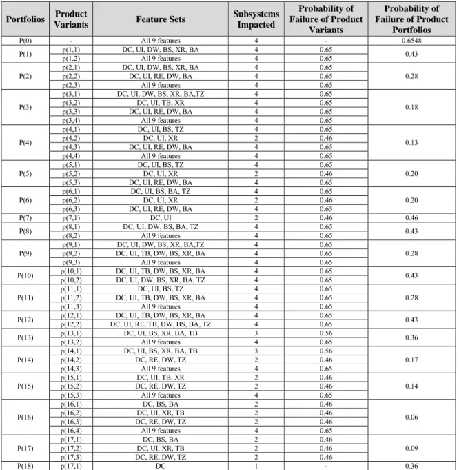
In this module, the human decision maker is gaining information related to the impact of the new features on ESS’s structure. jEdit v4.0 has thirty source code packages [31] [32]. Domain experts have identified four subsystems in jEdit’s structure [32]. Each subsystem consists of a group of packages and implements a subset of features. Table 4 lists the features that are implemented in each subsystem. The decision maker updates the feature sets of the product variants in the seven initially proposed SPL portfolios such that each product variants contains all the features corresponding to a given subsystem.
Table 4 Subsystems in jEdit’s system structure
Subsystem Corresponding Features
1 DC
2 UI, XR, TB
3 RE, TZ, DW
4 BS, BA
Table 5 shows the updates in the feature set of each product variant using the value of θadj equal to 50%. For example, for product variant p(1,1) of portfolio P(1), feature DW was removed
because the other features (TZ and RE) implemented by the subsystem 3 were not present in the feature set of p(1,1) (Section 4.3, Rule 3). TB was included in p(1,1) to complete the feature group corresponding to subsystem 2 (Section 4.3, Rule 2). The finalized structural-adjusted portfolios are P(13) to P(18) as shown in the Table A.1 (Appendix A) and Table B.1 (Appendix B).
Table 5 Structural adjustments to initial product portfolios
Portfolios Product
Variants Feature Sets Feature Removals and Additions
P(0) - All 9 features -
P(1) p(1,1) DC, UI, DW, BS, XR, BA, TB Removed DW and included TB
p(1,2) All 9 features -
P(2)
p(2,1) DC, UI, DW, BS, XR, BA, TB Removed DW and included TB p(2,2) DC, UI, RE, DW, BA, TZ Removed UI, BA and included TZ
p(2,3) All 9 features -
P(3)
p(3,1) DC, UI, DW, BS, XR, BA,TZ, TB, RE Included TB, RE
p(3,2) DC, UI, TB, XR -
p(3,3) DC, UI, RE, DW, BA, TZ Removed UI, BA and included TZ
p(3,4) All 9 features -
P(4)
p(4,1) DC, UI, BS, TZ, BA Removed UI, TZ and included BA
p(4,2) DC, UI, XR, TB Included TB
p(4,3) DC, UI, RE, DW, BA, TZ Removed UI, BA and included TZ
p(4,4) All 9 features -
P(5)
p(5,1) DC, UI, BS, TZ,, BA Removed UI, TZ and included BA
p(5,2) DC, UI, XR, TB Included TB
p(5,3) DC, UI, RE, DW, BA, TZ Removed UI, BA and included TZ P(6)
p(6,1) DC, UI, BS, BA, TZ Removed UI, TZ
p(6,2) DC, UI, XR, TB Included TB
p(6,3) DC, UI, RE, DW, BA, TZ Removed UI, BA and included TZ
P(7) p(7,1) DC, UI Removed UI
5.4
Module 3: Trade-off analysis
The third module of OPTESS performs trade-off analysis for all the candidate SPL portfolios. The candidate SPL portfolios include the initially proposed SPL portfolios given as input to OPTESS, the business-adjusted SPL portfolios, the technical adjusted SPL portfolios and the single software product. The trade-off is performed between two objectives: (i) minimizing the technical risk of failure due to implementation of features and (ii) maximizing the business values of the SPL portfolio.
5.4.1 Technical risk estimation
The technical risk of failure is calculated using Equation (5). The results are shown in Table 7 as probability of failure of the system when features are implemented in ESS’s structure. Note that for the jEdit case study we have access to data for only one of the parameters i.e. adjusted diffusion (ADF). The other four parameters in Equation (5) were ignored due to non-availability of data. Because of the incomplete data availability, we are not able to generate the values for the coefficients αi. Therefore, for this illustration we have applied the value of the coefficient α1 equal to 0.41 as suggested in [16]. It can be seen that the higher the number of subsystems impacted in ESS’s structure (reflecting higher diffusion) the higher the probability of failure. This activity of module 3, addresses RQ 2.
5.4.2 Cost estimation
The SIMPLE cost estimation model is applied (as explained in Section 3.1) to calculate the cost of developing the candidate SPL portfolios. The cost to calculate the unique part of each candidate SPL portfolio is estimated by identifying the features that are offered by only one of the product variants. These features will not be developed for reuse consequently the cost to implement them will be less as compared to the features that will be shared by multiple product variants. The SIMPLE model does not provide any details on how a particular cost function be estimated. As explained in Sections 2.3 and 3.1, we have applied an analogy-based effort estimation technique (AQUA) to estimate the function Cunique(). The effort estimate for implementing each feature of the jEdit software system is given in Table 1.
Development of shared features (determined by the Ccab() function), requires more effort. The reason is that these features will be shared by multiple product variants requiring implementation of variability mechanisms. The higher the level of variability amongst the product variants of a given SPL portfolio, the higher is the level of effort to develop them. If a feature is shared across all the product variants in a SPL portfolio, the effort estimate by AQUA is adjusted. This adjustment is based on the number of product variants that are sharing this feature and the number of packages being impacted by the feature in ESS’s structure. The interested reader is referred to [33] for detailed effort estimation results for shared features of each candidate SPL portfolio.
Adaption of a shared feature for use in a specific product variant requires some additional effort. This effort is reflected in the results of the function Creuse(). The actual value of the function Creuse() depends on how many product variants will be reusing the shared feature. Results for the function Creuse() for each candidate SPL portfolio in the jEdit case study are presented in [33]. The final cost estimates by application of the SIMPLE model for the single product and 18 candidate SPL portfolios are listed in Table B.1 (Appendix B). As mentioned in Section 4.4.2, Corg() cost function of SIMPLE is not applied in this case study.
5.4.3 Price and business value estimation
Prices are determined using the IR and IC constraints in Equations (2) and (3). The customer’s valuation of a product variant is calculated as the sum of all the feature voting scores that are no less than the threshold (6 in our case). Prices are set in such a way that customers can self-select their favorite product variants. Revenue is calculated by Equation (4) and business value is measured by Equation (6). To simplify the calculation of business value, we set the conversion factor β as 1.
Here we take P(1) as an example to show how business value of a specified SPL is calculated. Firstly, from the clustering results, we get that p(1,1) is designed for customers 1, 2, 3, 4, 5, 8, 9 and 10. Each customer’s valuation of p(1,1) is calculated as 29, 37, 44, 35, 40, 20, 32 and 32. To maximize revenue generated from p(1,1), we set price as 29. Because customer 8’s valuation for p(1,1) is 20, which is less than 29, according to the IR constraints, customer 8 will not purchase p(1,1). Accordingly, p(1,2) is designed for customers 6 and 7 with valuation 69 and 70. In order to encourage customers 6 and 7 to self-select p(1,2) instead of p(1,1), the IC constraints are applied so that the price of p(1,2) is set as 53. With this price schedule, customers 1, 2, 3, 4, 5, 9 and 10 purchase p(1,1) at price 29 and customers 7 and 7 purchase p(1,2) at price 53. Customer 8 does not purchase any product variant. The total revenue generated is 309. Using equation (1), we get the total cost associated with P(1) is 58.6. Thus the total business value for P(1) is calculated as 250.4. Table B.1 (Appendix B) lists the revenues and business values of all the candidate SPL portfolios.
5.4.4 Identification of non-dominated solutions
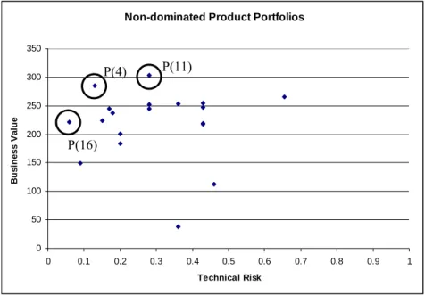
The decision maker is presented the business values and technical risk estimates for all the candidate product portfolios. Using this information, the non-dominated solutions can be identified. Non-dominated SPL portfolios perform better than all the other candidate SPL portfolios in the solution space when both the criteria are considered together. For the jEdit example, the portfolios P(4), P(11) and P(16) are the non-dominated solutions as identified in Figure 2. The decision maker analyzes the non-dominated solutions and selects the one of them.
Product portfolio P(4) is one of the initial product portfolios generated by cluster analysis using customers’ preferences on product features. This product portfolio does not have the highest business value amongst all the solutions nor the lowest technical risk. However, when both the objectives are considered together, it performs better than all the candidate product portfolios. The other two non-dominated solutions are the optimized solutions. Portfolio P(11) was optimized by performing business related adjustments, consequently it has the highest business value. Portfolio P(16) is optimized on technical objectives and thus has the lowest technical risk amongst all the candidate product portfolios.
Non-dominated Product Portfolios
0 50 100 150 200 250 300 350 0 0.1 0.2 0.3 0.4 0.5 0.6 0.7 0.8 0.9 1 Technical Risk B u si n ess V a lu e
Figure 2 Non-dominated product portfolios maximizing the business value objective and minimizing the technical risk objective
6
Applicability and Limitations
6.1
Applicability
Method OPTESS addresses the complex problem of evolving a software product facing feature demands of a diverse customer-base. The goal of OPTESS is to propose a portfolio of non-dominated solutions to the decision maker. These solutions can become a starting point for initiating discussions amongst project stakeholders.
In our previous works, we have proposed methods that can be applied for this decision problem of enhancing a single software product into a product line with different levels of data availability. In [30], we proposed method COPE (Customer Oriented Product Evolution) which requires information on customers’ preference structure on product features to determine
P(11) P(4)
segments of customers and suggests candidate SPL portfolios. A human decision maker is evaluates the candidate SPL portfolios using her expert judgment and selects a suitable portfolio for enhancing the ESS. The decision maker can also initiate further iterations of COPE by changing model settings to generate more solutions.
Method COPE+ [5] extends COPE by including impact analysis of the features on ESS’s architecture. The decision maker is given information on the level of impact of candidate SPL portfolios on ESS’s architectural components. COPE+ also performs behavioral comparison of candidate SPL portfolios and the ESS to rank the candidate solutions.
Method OPTESS brings in the economic consideration to ranks the candidate SPL portfolios using the technical and business objectives. This, however, requires more sophisticated data related to the impact of features on system structure, and effort estimates for implementation of features and pricing structure. Given such data requirements, we recommend the application of OPTESS for organizations being at least at CMMI level 3 where measurement and analysis practices are followed [34]. Tool support for the method OPTESS is also planned to automate some of the activities.
6.2
Assumptions and Threats to Validity
The assumptions and threats to validity of the work presented in this paper are listed below: (1) The risk estimates for the candidate SPL portfolios are calculated using data for only
one of the parameters in the Mockus and Weiss’s model [16]. This is a threat to the validity of the conclusions.
(2) Real customers were not involved for getting preferences on features of jEdit system. Therefore, no feedback is available to determine the level of acceptance for the results generated by OPTESS.
(3) For the jEdit system, we have used feature impact analysis results of [32] which can be a threat to the validity of conclusions.
(4) For revenue estimation, it is assumed that each customer buys one product. It may not always be true.
7
Discussion and Future Work
Creation of business value has always been advertised as one of the key benefits of a SPL development approach. Several case studies have been reported citing numerous business and technical benefits such as higher customer satisfaction, increase in productivity, reduction in maintenance costs, etc., [1] [2]. There is however, lack of scientific research, quantifying the economic value gained through adoption of a specific product line approach for a product. A panel discussion “How to maximize business return on SPL” was organized in the recent 13th International Software Product Line Conference (SPLC 2009) where practitioners and researchers called for conducting more research on how to define and increase business value from product
lines. A key conclusion was that value cannot be defined globally; it has to be defined for a
specific product line in a given organization [35]. Method OPTESS brings together the concepts and techniques from economics and software engineering to evaluate SPL portfolios for a given evolution scenario. The goal is to provide a decision support framework and not to focus on specific technical and economic techniques. The cost estimation model, risk estimation model and customer valuation technique applied in this paper are some example technique to show how trade-off analysis can be performed for selecting a candidate SPL portfolio.
In this paper we highlight the interplay between economic and technical aspects of the SPL design. In the economic side, we apply the widely adopted value-based pricing mechanism to estimate price and revenue in a self-selection market. The SIMPLE cost model is applied to estimate the effort for developing candidate SPL portfolios. On the technical side, a risk estimation technique is applied to determine the probability of failure of the system when new features are implemented. To balance both the economic and technical objectives, three non-dominated product portfolios were proposed out of eighteen candidate SPL portfolios.
Ahmed et al., have investigated on how some of the business factors influence success of SPLs [36]. They have argued that strategic planning is one of the key factors in business performance of a SPL. An important component of strategic planning is market orientation i.e., identification of customer segments and a plan to target them. There are other factors that are equally important e.g., competitors in each segment, order of entry in the market etc. OPTESS addresses a part of this strategic planning. Other techniques such as from marketing can be applied to bring in additional criteria for evaluation of the candidate SPL portfolios.
This paper presents initial results of our method on an open source text editing software system. In future, we plan to conduct a sensitivity analysis to identify the degree of influence of technical and economic factors on the results generated by OPTESS. Further case studies are planned with real customers to determine the level of acceptance of the results.
Acknowledgements
Guenther Ruhe would like to thank the Canadian NSERC Natural Sciences and Engineering Research Council (Discovery Grant 250343-07) for the financial support of this research.
References
1. P. Clements and L. Northrop, Software product lines: Practices and patterns, 3rd Ed., Addison-Wesley Professional, 2001.
2. F. Linden, K. Schmid, and E. Rommes, Software product lines in action: The best industrial practice in product line engineering, Springer-Verlag, New York, USA, 2007.
3. P. Clements, L. Jones, J. McGregor, L. Northrop, Getting there from here: A roadmap for software product line adoption, Communications of the ACM, 49(12), 2006, pp. 33-36.
4. M. Ullah, G. Ruhe, and V. Garousi, Towards design and architectural evaluation of product variants. A case study on an open source software system. In: Proceedings of the 21st International Conference on Software Engineering and Knowledge Engineering, USA, 2009, pp. 141-146.
5. M. Ullah, G. Ruhe, and V. Garousi, Decision support for moving from a single product to a product portfolio in evolving software systems, Elsevier Journal of Systems and Software, 2010, (submitted). 6. A. Helferich, K. Schmid, and G. Herzwurm, Product management for software product lines: An
unsolved problem? In: Communications of the ACM, 49(12), 2006, pp. 66-67.
7. G. Ruhe, Software engineering decision support – A new paradigm for learning software organizations. Advances in Learning Software Organization. Lecture Notes in Computer Science Vol. 2640, 2003, Springer, pp. 104-115.
8. E. Turban, J. Aronson, and T. Liang, Decision support systems and intelligent systems. Prentice Hall, 2004.
9. H. Rittel, and M. Webber, Planning problems are wicked problems. In: Cross N. (Ed.) Developments in design methodology. Wiley, Chichester, 1984, pp. 135-144.
10. P. Carlshamre, Release planning in market-driven software product development. Requirements Engineering Journal, vol. 7(3), 2002, pp.139-151.
11. C. Fritsch, and R. Hahn, Product line potential analysis, Proceedings of the 8th International Software Product Line Conference, LNCS 3154, 2004, pp. 228-237.
12. K. Schmid and I. John, Developing, validating, and evolving an approach to product line benefit and risk assessment, In: Proceedings of the 28th Euromicro Conference, Germany, 2002, pp. 272-283. 13. K. Schmid, A comprehensive product line scoping approach and its validation, In: Proceedings of the
24th International Conference on Software Engineering, ACM, New York, USA, 2002, pp. 593 – 603. 14. L. Bass, P. Clements, and R. Kazman, Software architecture in practice, 2nd Edition, Addison-Wesley
Professional.
15. B. Boehm, Software risk management: Principles and practices, IEEE Software vol. 8(1), 1991, pp. 32-41.
16. A. Mockus and D. Weiss, Predicting risk of software changes, Bell Labs Technical Journal, 5(2), 2000, pp. 169-180.
17. B. Boehm, Software engineering economics, IEEE Transactions on Software Engineering, vol. 10(1), 1984, pp. 4-21.
18. L. Northrop and P. Clements, A framework for software product line practice version 5.0, Software Engineering Institute, Pittsburgh, USA.
19. B. Boehm, A. Brown, R. Madachy, and Y. Yang, A Software Product Line Life Cycle Cost Estimation Model, In: Proceedings of the 2004 International Symposium on Empirical Software Engineering, ISESE'04, 2004, pp. 156-164.
20. H. In, J. Baik, S., Kim, Y, Yang and B. Boehm, A quality-based cost estimation model for the product line lifecycle, Communications of the ACM, vol. 49(12), 2006, pp. 85-88.
21. G. Boeckle, P. Clements, J. McGregor, D. Muthig and K. Schmid, A cost model for software product lines. Lecture Notes in Computer Science, vol. 3014, 2004, pp. 310-316.
22. L. Angelis and I. Stamelos, A simulation tool for efficient analogy based cost estimation. Empirical Software Engineering 5(2000), pp. 35-68.
23. M. Ruhe, R. Jeffery and I. Wieczorek, Cost estimation for web applications, Proceedings of the 25th International Conference on Software Engineering, Oregon, USA, pp. 285-294.
24. L. Angelis, I. Stamelos and M. Morisio, Building a software cost estimation model based on categorical data, Proceedings of the 7th International Symposium on Software Metrics, UK, 2001, pp. 4-15.
25. J. Li, G. Ruhe, A. Al-Emran, and M. Richter, A flexible method for software effort estimation by analogy, Empirical Software Engineering, 12(2007), pp. 65-106.
26. C. Shapiro and H. Varian, Information rules: A strategic guide to the network economy, Harvard Business School Press, 1999.
27. K. Moorthy, Market segmentation, self-selection, and product line design, Marketing Science, vol.3(4), 1984, pp. 288-307
28. A. Sundararajan, Nonlinear pricing of information goods, Management Science, vol. 50(12), pp. 1660-1673.
29. X. Wei and B. Nault, Product differentiation and market segmentation of information goods, Discussion Paper at the Workshop on Information Systems and Economics, Irvine, CA, 2005.
30. M. Ullah, and G. Ruhe, One product versus product line: Decision support based on customer needs analysis. In: Proceedings of the 11th International Conference on Software Product Lines, vol. 2, 2007, pp. 174-183.
31. jEdit Project Website., 2009. http://sourceforge.net/projects/jedit.
32. A. Kuhn, S. Ducasse, and T. Girba, 2007. Semantic clustering: Identifying topics in source code. Information and Software Technology, vol. 49(3), pp. 230-243.
33. http://pages.ucalgary.ca/~ullah/jEditCaseStudy.pdf
34. http://www.sei.cmu.edu/cmmi/tools/dev/index.cfm (Accessed July 5, 2010)
35. J. Bosch, K. Jackson, C. Krueger, J. McGregor, and A. Nolan, How to maximize business return of SPL, Goldfish Bowl Panel, 13th International Software Product Line Conference, August 2009, San Francisco, USA.
36. F. Ahmed and L, Capretz, Managing the business of software product line: An empirical investigation of key business factors, Information and Software Technology vol. 49(2007), pp. 194-208.
37. D. Muthig, J. McGregor, and P. Clements, Predicting product line payoff with SIMPLE, Tutorial in the 11th International Software Product Line Conference, Japan, 2007.
Appendix A
Table A.1 Probability of failure estimates for the candidate SPL portfolios
Portfolios Product
Variants Feature Sets
Subsystems Impacted Probability of Failure of Product Variants Probability of Failure of Product Portfolios P(0) - All 9 features 4 - 0.6548
P(1) p(1,1) p(1,2) DC, UI, DW, BS, XR, BA All 9 features 4 4 0.650.65 0.43 P(2) p(2,1) DC, UI, DW, BS, XR, BA 4 0.65 0.28 p(2,2) DC, UI, RE, DW, BA 4 0.65 p(2,3) All 9 features 4 0.65 P(3) p(3,1) DC, UI, DW, BS, XR, BA,TZ 4 0.65 0.18 p(3,2) DC, UI, TB, XR 4 0.65 p(3,3) DC, UI, RE, DW, BA 4 0.65 p(3,4) All 9 features 4 0.65 P(4) p(4,1) DC, UI, BS, TZ 4 0.65 0.13 p(4,2) DC, UI, XR 2 0.46 p(4,3) DC, UI, RE, DW, BA 4 0.65 p(4,4) All 9 features 4 0.65 P(5) p(5,1) DC, UI, BS, TZ 4 0.65 0.20 p(5,2) DC, UI, XR 2 0.46 p(5,3) DC, UI, RE, DW, BA 4 0.65 P(6) p(6,1) DC, UI, BS, BA, TZ 4 0.65 0.20 p(6,2) DC, UI, XR 2 0.46 p(6,3) DC, UI, RE, DW, BA 4 0.65 P(7) p(7,1) DC, UI 2 0.46 0.46
P(8) p(8,1) p(8,2) DC, UI, DW, BS, BA, TZ All 9 features 4 4 0.650.65 0.43 P(9) p(9,1) DC, UI, DW, BS, XR, BA,TZ 4 0.65 0.28 p(9,2) DC, UI, TB, DW, BS, XR, BA 4 0.65 p(9,3) All 9 features 4 0.65 P(10) p(10,1) DC, UI, TB, DW, BS, XR, BA 4 0.65 0.43 p(10,2) DC, UI, DW, BS, XR, BA, TZ 4 0.65 P(11) p(11,1) DC, UI, BS, TZ 4 0.65 0.28 p(11,2) DC, UI, TB, DW, BS, XR, BA 4 0.65 p(11,3) All 9 features 4 0.65 P(12) p(12,1) DC, UI, TB, DW, BS, XR, BA 4 0.65 0.43
p(12,2) DC, UI, RE, TB, DW, BS, BA, TZ 4 0.65
P(13) p(13,1) p(13,2) DC, UI, BS, XR, BA, TB All 9 features 3 4 0.56 0.65 0.36 P(14) p(14,1) DC, UI, BS, XR, BA, TB 3 0.56 0.17 p(14,2) DC, RE, DW, TZ 2 0.46 p(14,3) All 9 features 4 0.65 P(15) p(15,1) p(15,2) DC, RE, DW, TZ DC, UI, TB, XR 2 2 0.46 0.46 0.14 p(15,3) All 9 features 4 0.65 P(16) p(16,1) DC, BS, BA 2 0.46 0.06 p(16,2) DC, UI, XR, TB 2 0.46 p(16,3) DC, RE, DW, TZ 2 0.46 p(16,4) All 9 features 4 0.65 P(17) p(17,1) DC, BS, BA 2 0.46 0.09 p(17,2) DC, UI, XR, TB 2 0.46 p(17,3) DC, RE, DW, TZ 2 0.46 P(18) p(17,1) DC 1 - 0.36