Understanding Investment Incentives Under Parallel Tax Systems: An Application to the Alternative Minimum Tax

NEER WORKING PAPER SERIES

UNDERSTANDING INVESTMENT INCENTIVES UNDER

PARALLEL

TAX SYSTEMS:

AN APPLICATION TO ThE ALTERNATIVE MINIMUM TAX

Andrew B. Lyon

Working Paper No. 2912

NATIONAL BUREAU OF

ECONOMIC RESEARCH

1050

Massachusetts Avenue

Cambridge, MA 02138

March 1989

am grateful to Rosanne Altshuler, Don Fullerton, and Chuck Hulten for

elpful suggestions. This research is part of NBERs research program in

axation. Any opinions expressed are those of the author and not those of

I. Introduction

Concepts of investment incentives and investment neutrality are frequently analyzed by assuming all taxpayers are subject to a single statutory tax rate with _a fixed schedule of deductions and exclusions. However, most countries income _tax systems are more complex. Income tax systems generally provide a range of statutory tax rates, allowable deductions may be a function of income, and there _{may be} coordination between taxes paid over different points in time through a _{system of} tax credits, carrybacks, and carryforwards.

The tax rules which constitute a giyen income tax system may be thought of _as several parallel tax systems, any one of which may apply to a taxpayer at a given point in time. A taxpayer who is subject to these different parallel tax systems over time may face investment incentives very different from those faced by a taxpayer who is permanently subject to only a single tax system.

In the U.S. there are several examples of parallel tax systems. A graduated corporate income tax subjects income to four different tax rates ranging from 15 to 39 percent, while a firm in the highest income bracket is taxed at 34 percent. A firm with losses is subject to a zero tax rate and, if insufficient past tax liability exists, losses may be carried forward to offset future tax liability. Another parallel tax is the alternative minimum tax (ANT). As enacted in the 1986 Tax Reform Act, the corporate ANT has a statutory tax rate of 20 percent, its own depreciation schedules, and its own income exclusions. Taxpayers compute tax liability under both the regular tax provisions and the ANT, and they pay the larger amount. The extra taxes paid due to the ANT may be creditable in the future against regular tax liability.

A tax system (potentially encompassing multiple parallel tax systems) provides investment neutrality when two conditions are met. First, any asset with a given stream of receipts (before taxes) should be equally valued after taxes by different taxpayers. Second, different assets that are equally valued after taxes by a single

-1-taxpayer should offer the same pretax return.

If investment incentives are not neutral across assets and across taxpayers, the economy suffers real losses. The output attainable from the stock of capital could be increased if assets were reallocated, taxpayers, in an effort to mitigate burdens created by differential tax treatment, might be expected to engage in costly actions. Leasing, mergers, and delaying or accelerating the timing of investment are ways in which firms can achieve a lower cost of capital, while expending real

resources.

Standard propositions about how to achieve investment neutrality must be

reformulated when taxpayers are subject to different parallel tax systems over time. Consider the example of expensing. If taxpayers' tax rates do not change over time,

expensing (with no deductions for interest) satisfies the above conditions for investment neutrality. However, if tax rates change over time, expensing is not neutral. A taxpayer expensing an asset at a high initial statutory tax rate and

later subject to a lower statutory tax rate will face a lower required pretax return than another taxpayer permanently subject to either tax rate. Further, the first taxpayer will no longer be indifferent between assets with different rates of economic depreciation.

The next section shows that many parallel tax systems share common features and constructs a general model of the cost of capital based on the Hall-Jorgenson (1967)

cost of capital formula.

Section 3 presents conditions under which a parallel tax system maintains investment neutrality. In general, the neutrality conditions are sensitive to the assumed arbitrage conditions and source of finance.

Section 4 presents findings on the effect of the corporate ANT on investment incentives. It is shown that these investment incentives are sensitive to the length of time the firm is subject to the ANT, the timing of the Mt spell relative to the date the investment is acquired, and the source of financing. Investment

-2-incentives for firms experiencing temporary

spells

on the ANT can be very different

from those for firms permanently subject to the ANT.

The final

section briefly

summarizes the paper.

2.

Computing the Cost of Capital with a Parallel Tax

_System

The cost

of capital of an investment is the necessary pretax return the asset must

earn to justify its purchase. Derivations typically assume the taxpayer is

subject

to a constant statutory tax rate. If the taxpayer switches to a parallel tax system, however, the statutory tax rate may be different, depreciation

deductions may be different, and the firins discount rate may be different. In general, the cost of capital of a firm experiencing a spell on a parallel tax system is dependent on the duration of the spell, the time at which the investment is made,

and the source of financing.

To examine the effect of a parallel tax system on the cost of capital, the Hall-Jorgenson (1967) formula is modified to accommodate two tax systems -- a

"regular" tax system and a "parallel" tax system. For simplicity, the formula presented below considers a maximum of two switches between tax regimes. The firm

is assumed to be on the regular tax system from time zero to T1. At time T1 the firm switches to the parallel tax system. (If T1 —

, the

firm never exits the regular tax system. If T1 — 0, the firm starts on the parallel tax system.) At time T2 the firm returns to the regular tax system. The dates of switches between tax regimes CT1 and T2) are assumed to be known to the firm and independent of the marginal investment under consideration.1 If firms are uncertain as to the timing or duration of the spell on the parallel tax system, the cost of capital found for each possible pair of T1 and T2 must be weighted by its probability of occurrence.2

Earnings on the regular tax system and the parallel tax system are taxed at a statutory rate of u and rn respectively. Without any loss in generality, it is

assumed u > m.

or equity. Several arbitrage assumptions are possible to establish the equilibrium

rates of return for these sources of finance, but only one is considered here.

Following Bradford and Fullerton (1981), it is assumed that firms on the regular tax system are unconstrained in the amount of debt they may issue and arbitrage between debt and real capital. Therefore, firms on the regular tax system have a nominal after-tax discount rate of i(l-u). regardless of the source of finance, where i is

the pre-tax nominal interest rate on the firm's debt.3

Firms on the parallel tax system, however, have different discount rates for debt and equity. To derive their discount rate for equity, assume that individual

savers are indifferent between equity issued by firms on the regular tax system and by firms on the parallel tax system. Additionally assume that total investment undertaken by firms on the parallel tax system is small relative to that of other

firms. In this case, equity-financed investment must earn a return of i(l-u) for both types of firms. Denoting the equity-financed after-tax discount rate at time t

of firms on the parallel tax system by r, r —

i(l-u).

To derive the firms' discount rate for debt, assume that bondholders are indifferent between debt issued by regular tax firms and parallel tax firms. The pretax cost of debt finance is therefore i for both types of firms. If the parallel tax system provides a future tax credit for the extra taxes paid under the parallel tax system, such as under the ncr or tax loss carryforward rules, the after-tax discount rate of debt finance for a firm on the parallel tax system is time dependent. This is because interest payments are currently deductible at rate in, but the firm receives a tax credit of (u-m)i. The present value of this credit

depends on the time at which the credit may be claimed. The debt-financed nominal after-tax discount rate at time t is r—i(l-ni) -

_PV[(u-m)i].

where flY is the present

value operator from time t to the time at which the credit is claimed.4 A general expression for the cost of capital can be derived for firms experiencing a spell on the parallel tax system. The model applies with equal

-4-generality to a firm confronting a graduated rate structure •

a

_{loss firm with no}

carryback ability,5 or a firm on the ANT.

Assuming

that the cost of the asset is $1. the cost of capital c for the marginal investment is found by equating the asset's cost with the present value of

its after-tax earnings:

(1) $1 —

c ((1-u) J

ei16)tdt

T2

f

r.dT

+

(1-nOd J

e(2ö)te 1•T1

dt

*

(1u)e(utS)T2dd Je1_u48xt_T2)dt,

+ uZ (O,T )_{R 1} + md Z (T ,T )

_{1P 1}

₂

+

ud d Z CT ,)

_{12R 2}

+ d d ,

₁₂

where T2 -f

rtdt

-i(1-u)T

T

d

(2)

d —

e

1 and d —

1 are discount factors where r —

r

or r —

r

1 2 t

t

t

t.

it is

the rate of inflation and 6

is

the rate of economic depreciation;

(3) ZR(t,t) —

_DR(t)e

tt1)dt

where

DB(t) is

the allowable depreciation deduction under the regular tax system for the calendar year including t;

t

t2

-

₅

r7dr

(4) Z(t ,t) —

_Djt)

e dt, where

D(t) is the allowable depreciation deduction under the parallel tax system for the calendar year including t; and the tax credit for extra taxes paid on the parallel

(5)

—

V + W, where,

T2

V —

_u

S D (t) -

mE

D(t), and T1

T2

W — _{(rn-u) c J}

Or-Ut

at.

In eq. (1), the cost of capital c multiplied by the ten in braces represents the present value of the cash earnings of the asset, reduced by taxes paid on each tax regime the firm faces, and excluding depreciation allowances and tax credits. The next three terms reflect the present value of the depreciation allowances received under each tax regime, where ;(t1,t2) is the present value as of time t1 of depreciation allowances received until time t2 under the regular tax system and Z(t1,t2) is the corresponding expression under the parallel tax system. The present value of depreciation allowances are computed as shown in eqs. (3) and (4).

Finally, the term -y

in

eq. (1) reflects the tax credit received by the firm for the extra taxes paid on the parallel tax system relative to the regular tax

liability. The first component V is equal to (1) the after-tax value of the

depreciation deductions the firm would have received had it been on the regular tax system, reduced by (2) the after-tax value of the depreciation deductions received under the parallel tax system. W is the tax savings from the reduced taxation of

the direct earnings of the asset while the firm was on the regular tax system. It is assumed that the credit may be claimed in full the year the firm returns to the regular tax system.6 Any statutory limit on the number of years the tax credit may be carried forward is incorporated into the T1 of eq. (5)2

Other special provisions of the parallel tax system pertaining to investments may also be incorporated. For example, beginning in 1990 under the ANT, a special tax is imposed on 75 percent of the difference between the ANT depreciation

deduction and a depreciation deduction calculated using yet another depreciation schedule. The amount of this tax would be subtracted from eq. (1) (with proper

-6-discounting) and added to the tax credit shown in eq. (5).8

Letting t represent the term in braces in eq. (1), the cost of capital _c can be solved as

I - uX _{(O,T )-md Z (T ,T )-ud d Z (t ,.)}

_{- Vd}

_d

(6) c — R

t + Wd1d1

1 2 It 2 1 2

As a special case, if the firm is always subject to the regular tax

system (T1 —

_{øo), eq.}

(6) simplifies to the traditional Hall-Jorgenson cost of capital formula, (i(l-u) -

r

_{+ 6)(l.uZ(O,c))}

(7) c—

1-u

If the firm is always subject to the parallel tax system (T1 — _{0 and T2 —}

_{co), then}

(r -

r

_{+ 5)(] -mZ (0,.))}

(8) c —

i

- _m

where r —

i(l-u)

or r —

_1(1-rn)

_{if the investment is financed with equity or debt,}

respectively.

3. Invariant Valuation under a Parallel Tax System

Samuelson (1964) proved that if and only if depreciation for tax _{purposes is} equal to economic depreciation will any two taxpayers with different tax rates value an asset equally. Sarnuelson referred to this condition as invariant valuation, that is. the valuation of an asset with a given stream of receipts is independent of the tax rate of the individual. Samuelson's proof was only for the case of taxpayers with different, but constant, tax rates. As noted by Sarnuelson,

All of this analysis presupposes a tax rate that is uniform over time for each person. Obviously, if a man is to be subject to different rates, with (the tax rate] being a function of time, his optimal decision will be distorted by this fact. A proper system of forwards and carry-backs, which makes Ithe tax rate] average out to a constant and which

takes account of just when a man pays the tax accruing to him, will avoid such

Under a parallel tax system, taxpayers' statutory tax rates _{may change over} time. The conditions under which invariant valuation is maintained in the _presence of a parallel tax system is examined in this section. Several possible solutions to

First, it is shown that even if taxpayers switch between a parallel tax system and the regular tax system, economic depreciation under both tax systems yields

invariant valuation if Samuelson's assumption on discount rates is maintained. (Given the arbitrage assumption of section 2. this corresponds to the condition that the investment is financed with debt.) That is, no tax credits, carryforwards or carrybacks are required, unlike Samuelson's presumption in the above quote. If

taxpayers' discount rates are set in a manner other than that assumed by Samuelson (for example, if equity finance is assumed), economic depreciation does not result in invariant valuation for taxpayers whose tax rates differ either permanently or temporarily. The necessary relationship between depreciation on the regular tax system and parallel tax system for invariant valuation in this case is also shown.

Second, if the extra tax paid while on the parallel tax system is creditable with interest against tax due on the regular tax system, then valuation will be invariant for any method of depreciation under each tax system.

third, it is shown that while expensing (with no interest deductions) leads to invariant valuation when tax rates are constant, valuation is not invariant when tax

rates change over time, In other words, expensing is fl2.t neutral, even if both the

regular tax system and the parallel tax systems have expensing, if the statutory tax rates differ. A depreciation system with the same present value as expensing, however, can be designed that does result in invariant valuation.

3.1 Economic Deoreciation

When taxpayers have diffeçent, but constant, tax rates others have shown

(Samuelson (1964), King (1975), Bradford (1981)) that invariant valuation results if interest payments are deductible and depreciation deductions are equal to economic depreciation.'° This solution also holds under a parallel tax system when tax rates

change over time.

Samuelson, King, and Bradford assume that the after-tn discount rate of an

I

investor

is equal to the interest rate times one minus the investor's tax rate.

This corresponds to the notion of debt-financed investment by firms on a parallel tax system with no tax credit. In this case, the after-tax discount rate on the regular tax system and parallel tax system is i(1-u) and i(l-m), respectively.

Lyon (1989) presents a general proof of invariant valuation with economic depreciation and this discount rate assumption when statutory tax rates change over time. Under the assumption of exponential economic depreciation, invariant

valuation can be shown by appropriate substitution into eq. (1). If Dt) —

_D,(t)

—

— i(l-m),

and — 0, then c —

I

- _{w + 6 independent of T and T.}

The cost of capital c is the same for all taxpayers independent of the timing and number of switches to the parallel tax system. Equality of the cost of capital across taxpayers for a given asset is a necessary and sufficient condition for

invariant valuation. 11

Thus given this discount rate assumption, parallel tax systems with different statutory tax rates need not rely on tax credits to achieve invariant valuation if all parallel tax systems provide economic depreciation.

The special assumption required for this result is that after-tax discount rates vary by a factor of one minus the investor's tax rate. Under the assumption of equity-financed investment, firms on the regular tax system and parallel tax system will have equal after-tax discount rates. In this case, economic

depreciation will not result in invariant valuation. If economic depreciation is exponential, however, a relationship between depreciation on the regular tax system and depreciation on the parallel tax system can be established that does result in invariant valuation for this and alternative discount rate assumptions.

Specifically, if the depreciation allowances under the regular tax system are proportional to the replacement cost of the asset, a depreciation schedule for the parallel tax system exists that will provide invariant valuation independent of the duration and number of spells on the parallel tax system.

to the replacement cost of the asset need not be considered overly restrictive, as any desired effective tax rate can be attained under

such

a system. specifically. let the depreciation deduction at time t

under

the regular tax system DR(t) be

*

(x-6)t

(9)

D(t)

—

8 e

• where

10'/ 8* & +

(i(l-u)-ff)(l-a)

1-au

In this case, an equity-financed investment by a firm permanently on the regular tax system will have an effective tax rate of cu, i.e., the cost of capital

c_[i(l-u)-w)/(lau) +

8.

By choosing a, any desired effective tax rate can be

determined.

For equity-financed investment of firms on the parallel tax system, invariant valuation will result if the depreciation deduction at time t under the parallel tax

system D(t) is

(11)

D(t) —

se0flt,

where (12) 6' —

c(mu)+

u8*

and where c is the cost of capital for a firm on the regular tax system)-2 With these depreciation schedules, the cost of capital c for a project undertaken by a firm permanently on the regular tax system will be equal to that of a firm subject to the parallel tax system at any point in time. (The proof of this result is given

in Appendix B.)

Under the systems of depreciation allowances given by eqs. (9) and (11), the reduction in tax liability on the cash earnings of the asset to the firm on the parallel tax system is exactly offset at each point in time by the reduced after-tax value of the depreciation deductions. As a result, the tax credit owed to a firm exiting the parallel tax system for the regular tax system is zero from this

investment. The tax credit can therefore be eliminated and not alter the solution. A general relationship between 6' and 6* can be shown to exist for any assumed relationship between the after-tax discount rate of firms on the regular tax system

-10-and firms on the parallel tax system. In the absence of a tax credit for taxes paid

on the

parallel tax

_system,

cOn-u) + u8*

+

_rp

-

_rR

(13)

8'—

where rR is the nominal after-tax discount rate for firms on the regular tax system and

r, is the nominal

after-tax

discount rate for firms on the parallel tax

systemJ3 Thus, alternative discount

rate assumptions will result in different depreciation

allowances. In the case considered by Samuelson and others where

rR—i(l-u)

and then

c—i+6-,r. Substituting these values in eq. (13) with

r—i(1-m),

yields 6'—6-w. Decreases in r. such as in the case of equity finance, will require reductions in 8' relative to

_{economic depreciation in}

_order

_{to maintain}

invariant

valuation.

The requirements for depreciation on the parallel tax system to achieve invariant valuation when depreciation on the regular tax system is proportional to economic depreciation are given by eq. (13). The obvious drawback of these

relationships is that tax authorities are required to distinguish whether an investment is financed by debt or equity for firms subject to the parallel tax system. Since this distinction may not be practical, methods of achieving invariant valuation that are independent of the source of finance are examined in the

remainder of section 3.

3.2

Interest Bearina Tax Credits

If

the value of the tax credit earned on the parallel tax system were increased

at the nominal after-tax discount rate of firms on the regular tax system. QiIX pair

of depreciation schedules under the parallel tax system and the regular tax system will result in invariant valuation, provided the credit is eventually claimed.

Clearly, if firms on the two tax systems have the same after-tax discount rate (as

is assumed in the case of equity-financed investment) this result must obtain

because

the present value of the

taxes paid from a given investment will be equal.

-11-This result also will hold for debt-financed investments, because, with a tax credit of this form, the debt-financed discount rate of a firm on the parallel tax system is equal to that of a firm on the regular tax system.14

Invariant valuation may be shown by rewriting the ten reflecting the tax credit (the term y

in

eq. (5)) for T2Cc as:

—

(V'+

W') where, V1 — tlZ7(( -

rnZ(T1.T2).

and T2 — _(rn-u) c j'

Substitution into eq. (1) after cancellation of tens yields

(1') $1 —

c

((lu)Je

(i(lu) lrl-a)tdt)

_{+ uZR(O.Tl)}

+

udZ(T

,T) +

_uddZR(T2).

After simplifying the terms involving ZR. it can be seen that the cost of capital c is the same as for a firm permanently on the regular tax system. Allowing the firm to earn interest on its tax credit equates the present value of taxes paid by the firm with that of a firm permanently on the regular tax system.

In the previous section it was shown that invariant valuation requires that depreciation deductions on the parallel tax system be determined in a manner

dependent on the source of finance. Only an interest bearing tax credit will ensure invariant valuation for any pair of depreciation schedules and independent of the source of finance, if interest deductibility is maintained.15

3.3 Enensina

King (1975), Bradford (1981), and others have shown that when taxpayers have different, but constant, tax rates a system of expensing (in the absence of a deduction for interests payments) will lead to invariant valuation. With a parallel

tax system, however, this result no longer obtains. Firms that expense the asset oil the regular tax system (the system with the higher statutory tax rate) and later

-12-switch to the parallel tax system will have a lower cost of capital than firms permanently subject to a single tax system. Similarly, firms that expense the asset

on the parallel tax system and later switch to the regular tax system will have a higher cost of capital.

This can be seen as follows, With no interest deduction, all firms have the same discount rate i independent of the source of finance. For a firm always under only one tax system that expenses an asset, the present value of the pretax earnings of the asset is $1. since (from eq. (1))

(14) $1 —

cf

eS)tdt.

For any finite duration from time zero to 1, the present value of the pretax

earnings must be less than $1. But the pretax value of expensing the asset at time zero is exactly $1. Since this is greater than the earnings of the asset over the initial tax regime, the firm will have a lower cost of capital if it expensed the asset at the higher statutory rate of the regular tax system and then switched to the parallel tax system. Similarly, the firm will have a higher cost of capital if the order of the tax regimes is reversed. This occurs whether or not a

(non-interest bearing) tax credit is provided.

Expensing, therefore, is no longer neutral for firms experiencing spells on the parallel tax system of different durations. Further, for a single firm experiencing a spell on the parallel tax system, expensing no longer results in neutral

investment incentives for assets with different rates of economic depreciation. Table 1 summarizes the effects of switches between parallel tax systems on the cost of capital under systems of expensing and economic depreciation.

Neutrality can be restored, however, if a particular depreciation schedule is used on both the regular and parallel tax systems with the same present value as expensing. This may appear contrary to most suppositions that only the present value of depreciation allowances affects the cost of capital. When tax rates change over time, however, the value of a given deduction is dependent on the tax rate at

that point in time.

If depreciation deductions on both the regular and parallel tax systems at time t are equal to (5+i.r)e(T6)t, then firms permanently on, or switching between, tax systems will have a cost of capital c equal to i+5-?, the same as if the asset were expensed. In this case, pretax cash earnings from the asset at time t are equal to

ce(1S)t —

_{(i÷&.w)e(N&)t.}

Because at each point in time these earnings are equal to the depreciation deduction, no taxes are paid on the income generated by the asset. This result is independent of the tax rate. Therefore, firms switching between, tax systems have the same cost of capital as firms permanently subject to

either tax system.16

4. Investment Incentives under the ANT

This section examines the effect of a particular parallel tax system, the ANT, on investment incentives. The ANT

is

a parallel tax system with its own statutory

tax rate, depreciation schedules, allowable deductions, and tax exclusions. A corporation calculates its tax liability under both the regular tax system and the ANT, and pays the greater amount. Extra tax paid on the ANT due to timing

differences between the two tax systems is creditable in the future against regular tax liability. Dworin (l987b) estimates that at least 20 percent of all

corporations with book income exceeding $1 million are subject to the ANT. Differences in the computation of alternative minimum taxable income and regular taxable income for corporations arise in the treatment of both deductions and income. Deductions may be reduced under the ANT for depreciation, mining exploration and development costs, intangible drilling costs, percentage depletion, and charitable contributions of appreciated property. Reported taxable income is accelerated under the ANT for the completed contract method of accounting and the installment method of accounting. Additionally, interest on certain tax-exempt bonds is taxable under the ANT.

While the existence of the ANT cannot lower a firm's total tax burden (or lower

-14-its averafe effective tax rate), the effect on marginal investment incentives is not immediately evident. Assets generally receive less accelerated depreciation

deductions under the ANT than under the regular tax system, but income from the asset is taxed at a statutory rate of only 20 percent under the ANT versus 34 percent under the regular tax system. As shown in section 3, only in very special cases is it expected that the ANT would leave investment incentives unchanged,

Also evident from the discussion in section 3 is the importance of considering the duration that a firm is subject to the parallel tax system when considering its incentive and efficiency effects. Several analysts have examined only the case of firms permanently subject to the ANT. Unfortunately, the cost of capital for a firm temporarily subject to the ANT is not a weighted average of the cost of capital of firms permanently subject to the regular tax system and the parallel tax _system. Therefore, conclusions drawn from studies examining permanent ANT liability may not apply in the more likely case of temporary ANT liability.

For example, Graetz and Sunley (1988) find, for a firm permanently subject to the ANT, investment incentives are greater for most equity-financed investments relative to those of the regular tax system. For debt-financed investments they find the opposite effect. Not considered by Craetz and Sunley is the effect on investment incentives if a firm is only tenrnorarily subject to the ANT. This case is likely to be far more prevalent. As shown below, some of the findings of Graetz and Sunley can be reversed in the case of temporary ANT liability.

In considering the efficiency effects of the ANT, Bernheim (1989) finds that for a firm permanently subject to the ANT its choice of investment may be less distorted by tax considerations than if the firm were permanently subject to the regular tax system. Under the ANT, depreciation more closely approximates estimates of economic depreciation. Firms permanently subject to the ANT face less variation in the cost of capital (net of depreciation) across diverse assets. Bernheim therefore suggests that the ANT may actually improve economic efficiency.

Bernheim's finding, however, can also be reversed in the case of firms only teanorarily subject to the ANT. Thus, the ANT can increase the variation in the

cost of capital faced by a single firm.17

Firms with a higher cost of capital on the ANT than firms on the regular tax system are likely to reduce investment and engage in tax-motivated merger or leasing transactions to lower their cost of capital. There is some evidence that firms disadvantaged by the ANT have increased their use of leasing.18

In this section, the effect of the ANT on investment incentives is examined by comparing the cost of capital for a firm experiencing spells on the ANT of various lengths to the cost of capital for a firm permanently on the regular tax system.

Calculations of the cost of capital are based on eq. (6). Eq. (6) is modified to account for the adjusted current earnings preference of the ANT.19 The adjusted current earnings preference imposes a tax on 75 percent of the difference between ANT depreciation and the least accelerated of (I) straight-line depreciation over the asset's recovery period under the alternative depreciation system or (2) the depreciation method used for financial reporting. The method which is least accelerated is determined by a comparison of the present values of depreciation allowances under the two methods. It is assumed here that the straight-line

depreciation method over the alternative depreciation system recovery period is less accelerated than the method used for financial reporting.2°

The cost of capital model is calculated in discrete, rather than continuous, time. As explained in section 2, for firms subject to the ANT for finite periods

the nominal after-tax discount rate for debt-financed investment, r, is time

dependent. As a result, discount factors for periods the firm is subject to the ANT

may not be derived analytically in continuous time.

With eqs. (1) -

(6)

reformulated in discrete time, parameters may be set for the variables. The after-tax nominal discount rate for equity-financed investment,

i(1-u), is set equal to .09. This is also the discount rate for debt-financed

-16-investment for firms subject to the regular tax system. The inflation rate ,r is set so that the real after-tax discount rate for firms on the regular tax system is

equal to .05. (In discrete time, [l+i(l-u)]/(1.i-w) -l —

_.05)

The inflation rate is

approximately .038.

The cost of capital net of depreciation is reported for the aggregate

categories of equipment, structures, intangible capital, inventories and land, and total corporate capital. The cost of capital for equipment is based on a weighted average of the cost of capital of 31 different types of equipment. The structures aggregate is a weighted average of residential and commercial buildings. Intangible capital is a weighted average of research and development (R&D) and advertising.21

Under the 1986 tax law, recovery periods for equipment under both the regular tax system and the ANT are generally a function of the assets Asset Depreciation Range (ADR) midpoint (an estimated service life). Recovery periods under the regular tax system are up to 50 percent shorter than the ADR midpoint. Most

equipment on the regular tax system is recovered using 200 percent declining balance switching to straight-line. Long-lived equipment (essentially public utility equipment) is recovered using iSO percent declining balance switching to

straight-line.

Recovery periods for equipment under the ANT are generally equal to the asset's ADR midpoint. Depreciation deductions for equipment are calculated using the 150 percent declining balance method switching to straight line.

Structures are depreciated using the straight-line method under both the regular tax system and the ANT. Under the regular tax system, the recovery period is 27.5 years and 31.5 years for residential and commercial buildings, respectively. Under the ANT, both types of structures are recovered over 40 years.

Intangible investments are expensed in the year of purchase under both tax systems. Finally, land and inventories are not depreciated.

depreciation rates determined by }iulten and Wylcoff (1981). Hulten and Wykoff

suggest that annual rates of economic depreciation for equipment may be approximated by the relation 6 —

l.65/T,

where T is the asset's life as calculated by the Bureau of Economic Analysis (BEA). Based on an approximate relation between SEA lives and ADR midpoints, depreciation rates in this study for equipment are calculated as 6 —

l.25/L,

where L is the asset's ADR midpoint. Depreciation rates for residential and

commercial buildings are assumed to be .031. Additionally, R&D and advertising are assumed to have annual rates of depreciation of .15 and .33, respectively.

The following sections present the cost of capital for four different possible cases. In the first two cases, the cost of capital for a firm permanently subject to the regular tax system is compared to the cost of capital for a firm permanently subject to the ANT. The third case is of a firm experiencing an initial spell of finite duration on the ANT after which the firm returns to the regular tax system. The fourth case is of a firm initially on the regular tax system that switches to the ANT for a finite time period, and then returns to the regular tax system. The cost of capital under each of these four cases can be very different, and also differs depending on the source of financing for the investment. For each of the cases, equity-financed investment is examined first, followed by debt-financed

investment.

4.1 Case 1 end 2: Permanent Repular Tax and Permanent ANT Liability A. Equity Finance

The cases of firms permanently subject to the regular tax system and

Permanently subject to the ANT are presented first. As may be seen by comparing eqs. (1) and (8), the cost of capital for a firm permanently subject to the ANT is less than the cost of capital for a firm permanently on the regular tax system if and only if

I-u l-rnz (0,)+ACE (15)

(j—)( l-uZ(0,)

)

< 1.

-18-where the term ACE is included to represent the present value of the extra tax paid on the investment due to the adjusted current earnings preference. In general, there is a tradeoff between the lower tax rate at which earnings from the marginal investment are taxed on the ANT and the less accelerated rate at which depreciation may be taken under the ANT (as well as the extra tax incurred as a result of the

adjusted current earnings preference).

For investments that are either expensed or not depreciated, eq. (15) is easily evaluated. For inventories and land, which are not depreciated, the left-hand side of the equation reduces to (l-u)/(l-m), which is less than 1. Thus, the cost of capital of these investments is always lower for a firm permanently subject to the

MT.

The effective tax rate for inventories and land is equal to the statutory tax rate under each tax regime. For investments in intangible capital, which are

expensed, the left-hand side of the equation reduces to 1. The cost of capital of intangible capital is identical for firms permanently subject to each tax regime. The effective tax rate for intangible investments is zero.22

For other assets, the present value of depreciation allowances under each tax regime and the adjusted current earnings preference must be explicitly calculated. Given Z, Z, and ACE, it can be determined whether the cost of capital for a firm permanently subject to the ANT is higher or lower than the cost of capital on the regular tax system. As can be seen from eq. (15), the result is independent of the actual economic rate of depreciation for the asset.

The cost of capital net of depreciation of the different capital stock

aggregates for firms permanently on the regular tax system is shown in column (1) of table 2. The cost of capital for equipment is 6.8 percent, corresponding to an effective tax rate of 27 percent. Structures, with less accelerated depreciation, have a cost of capital of 7.7 percent. This corresponds to an effective tax rate of 35 percent, just exceeding the 34 percent statutory tax rate. Investments in

7.6 percent cost of capital. The average cost of capital for all assets weighted by

capital stock is 7.1 percent.

The cost of capital for firms permanently subject to the ANT is shown in column (2) of table 2. For the equipment category, the cost of capital is 6.5 percent. about 5 percent lower than under the regular tax system. The cost of capital for structures on the ANT is 6.5 percent, about 16 percent lower than under the regular tax system. Intangible capital has a cost of capital of 5 percent under both tax systems. Nondepreciable inventories and land have a cost of capital of 6.25 percent under the ANT. The average cost of capital for all assets under the ANT is 6.2 percent. The standard deviation in the cost of capital for firms permanently subject to the ANT, shown in the last row of column (2), is almost one-half that

found for the regular tax system.

The general findings of Graetz and Sunley and Eernheim are replicated in the computations shown in table 2. The cost of capital of firms permanently subject to the ANT is generally lower than under the regular tax system and the variation in the cost of capital across diverse assets is reduced. This analysis might

incorrectly suggest that in all cases the ANT's effect on investment incentives is relatively modest and that it may even increase investment incentives. This is true only for most equity-financed investment of firms Dermanently subject to the ANT. As shown in section 4.2, however, if firms undertake the investment while subject to

the ANT and expect to remain on the ANT only temporarily, investment incentives can be adversely affected. Further, as shown below, if the marginal investment is

debt-financed, a firm permanently subject to the ANT has a significantly higher cost of

capital.

B. Debt Finance

A firm permanently subject to the ANT financing an investment with debt has a nominal after-tax discount rate of i(l-m), while the discount rate for firms on the regular tax system is i(l-u) for both equity and debt finance. The higher cost of

-20-debt finance for a firm

_permanently

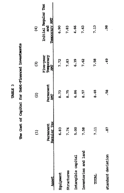
_{on the ANT presents a significant impediment.} Column (2) of table 3 shows the cost of capital for debt-financed

investments permanently subject to the ANT. The cost of capital for equipment and structures

is

8.7 percent. The average cost of capital for all assets is 8.5 _percent.

This cost of capital is 36 percent higher than the cost of _{capital for ANT} firms using equity finance. Relative to regular tax firms, the ANT _{cost of capital} is higher for all assets, including intangible capital1 _{inventories, and land. A} firm permanently on the ANT required to borrow to finance investment _{will have a} significantly higher cost of capital than a firm on the regular tax

system.

4.2. case 3: Terorary Initial MIT Liability

The cost of capital for a firm initially subject to the ANT that later _returns to the regular tax system is presented in this section. The discussion below

examines investments financed with equity first, followed by debt finance.

A, Equity Finance

To help understand the multiple channels by which an extended duration _{on the} ANT affects the cost of capital, equity-financed investments in

inventories, land, and intangible capital are considered first. Because inventories and land _{are not} depreciable, there is no difference in the after-tax value of deductions taken under the ANT and no tax effect from the adjusted current earnings preference. _Income generated by these assets while the firm is subject to the ANT is taxed at a rate of 20 percent instead of 34 percent. The current tax savings on this _{income, however,} results in an equal reduction in the fin's ANT credit. The ANT credit _{generated by} investment in inventories and land is negative, and offsets the positive ANT credit from the firm's other activities. Because the ANT credit is claimed at a later date, the present value of taxes paid by the firm is lower. As the duration on the

ANT

_increases,

_{the cost of capital for these assets declines further. The}

longer the firm

is

_{subject to the ANT, the greater is the reduction in the present value of}

-21-taxes paid.

The effect of the ANT on equity-financed intangible capital follows the

analysis of expensing in section 3.3, summarized in table 1. It was shown that if the firm purchases an asset while subject to the parallel tax system and the firm later switches to the regular tax, the cost of capital is higher than if the firm were permanently subject to either tax

_regime.

The gain from the deferral of taxes on the investment's earnings is less than the loss from the deferral of a portion of the deduction for the cost of the investment, It is interesting to note that

investment in intangible capital can be deterred even though there is no explicit

penalty for such investments under the ANT for corporations.

The effect of finite initial periods on the ANT

for

investment in

equity-financed depreciable assets introduces more complications because, in addition to the difference in statutory tax rates in each regime, depreciation schedules differ and tax may result under the adjusted current earnings preference. The basic principles, however, are similar to those applying to inventories and intangible

investments.

Column (3) of table 2 shows the cost of capital of a firm that will be on the ANT for the first five years of a contemplated investment, after which the firm will

be subject to the regular tax

_system.

Equipment has a cost of capital of 7.4 percent, higher than if the firm

were

permanently subject to either tax system. Structures, on the other hand, have a cost of capital lower than under the regular tax system. Intangible capital has a cost of capital of 6.0 percent, 20 percent higher than if the firm were permanently subject to either tax system. Inventories and land have a cost of capital slightly

lower than permanent regular tax liability. The average cost of capital for all

assets is 7.4 percent.

B. Debt Finance

Debt-financed investments of firms initially subject to the ANT

bear

a

-22-uniformly higher cost of capital than for firms

_permanently

_{on the regular tax} system. The cost of capital is also higher than for equity-financed investments _of ANT firms. The disadvantage ef debt financing relative to

equity financing

increases with the length of time on the ANT. For initial durations of _{one or two} years the disadvantage is slight, as the after-tax cost of debt finance after

receipt of the ANT credit is nearly equal to that of equity finance. For longer spells, the discount rate over the initial periods approaches i(l-m).

The cost of capital for a firm subject to the ANT for the first five _{years of} an investment is shown in column (3) of table 3. A five-year spell on the ANT increases the firm's nominal after-tax discount rate from 9 percent to 9.7 percent in the first year. The discount rate declines steadily in the next four

years.

Compared with an identical firm using equity finance (column (3) of table 2), the cost of capital is only slightly higher with debt finance. The cost of capital of all assets is also higher than for a firm permanently subject to the _{regular tax}

sys tern.

4.3. Case 4: Te'orary Initial Itepular Tax Liability

The cost of capital for firms initially on the regular tax system that later experience a spell on the ANT is very different from the cost of capital found in the previous cases. In general, the effects on the cost of capital are dependent on the durations on each tax system. As an example of the possible effects, the cost of capital is calculated for a firm assumed to have an initial period of regular tax liability of three years, after which it experiences a five-year period of ANT liability. The firm then returns to the regular tax system. Equity-financed investment is examined first, followed by debt-financed investment.

A. Batty

Finance

In section 3.3 it was shown that fins that expense equity-financed investments while subject to the regular tax and that later switch to the ANT have a lower cost

-23-of capital than if they remained on the regular tax system. For depreciable assets it is clear that the same result can occur if depreciation deductions under the regular tax system are exhausted before the firm switches to the ANT with the lower statutory tax rate. (Additionally, the firm nay be eligible to receive further depreciation deductions under the ANT or

tax

reductions due to the adjusted current earnings preference). It may be surprising, however, that even after short periods of regular tax liability, a duration of ANT liability can result in a lower cost of

capital.

The cost of capital for equity-financed investments is shown in column (4) of table 2. All assets are shown to have a lower cost of capital in this case than if the firms were permanently subject to the regular tax system. The largest reduction in the cost of capital occurs for intangible capital. The cost of capital for this asset is 4.5 percent, or an effective tax rate of -11 percent.23 The average cost

of capital for all assets is 7.0 percent.

As noted earlier, Bernheim (1989) suggests that the reduced dispersion in the

cost of capital for firms permanently on the AlIT may help improve economic

efficiency. But for firms that first experience a period on the regular tax system before a later spell on the ANT, the variation in the cost of capital can be

greater. As shown in table 2, the standard deviation in the cost of capital in this case is higher than for firms permanently subject to the regular tax system. For

firms experiencing these types of spells, investment decisions may be more distorted

than under the regular tax system.

B. Debt Finance

The higher cost of finance for debt finance increases the cost of capital relative to equity finance. Column (6) of table 3 shows the cost of capital for this case. The cost of capital is higher for the aggregate categories of equipment, structures, and inventories and land than for permanent regular tax liability. The cost of capital for intangible capital, however, is lower.

As found above for equity finance, the variation in the cost of capital for firms with initial periods of regular tax liability is greater than for firms permanently subject to the regular tax system.

5. Conclusions

This paper has shown the potential for taxpayers to face widely varying investment incentives when they are subject to different statutory tax rates and depreciation systems over time. A tax system can provide neutral investment incentives for a taxpayer permanently subject to a single statutory rate, but very unequal investment incentives for other taxpayers.

Neutral parallel tax systems can be designed in several ways. Economic

depreciation on each parallel tax system provides neutrality only if all firms have discount rates associated with the use of debt finance. If discount rates of firms are different from that assumed in the case of debt finance and if economic

depreciation is of an exponential form, other relationships between the required depreciation allowances on each parallel tax system can be established. The most general solution which provides neutrality under any system of depreciation allowances, any source of finance, and any form of economic depreciation is a tax credit that increases in value at the after-tn discount rate of firms on the regular tax system. All that is required is that the tax credit be eventually

claimed.

With

_regard

to the ANT

it

was shown that firms

_subject

to the ANT _may have either a higher or lower cost of capital than firms permanently on the regular tax system. The cost of capital for firms experiencing a spell on the ANT is sensitive to the duration of the spell, the timing of the spell relative to the date the investment is acquired, and the source of financing.

Firms on the ANT for short durations are likely to have a higher cost of

capital for most equipment. On the other hand, a firm purchasing equipment or other assets while on the regular tax that later switches to the ANT is likely to have a

lower cost of capital. Investment for which no explicit ANT penalty exists, such as

intangible capital, may be affected by the ANT as m'.sch as depreciable capital.

Firms on the ANT financing investments with debt face a higher cost of capital than identical firms that use equity financing. The disadvantage to debt finance

increases with the duration the firm is subject to the ANT.

-26-1. _{Because the formula derives the cost of capital for a small,}

marginal investment, these dates are assumed not to change if the marginal investment

occurs.

Auerbach (1986) examines the effect of inframarginal investment _{on the probability} that a firm will have tax losses. In his model, however, capital lasts

only one period. Dworin (1987a) studies the effect of inframarginal investment on ANT liability, but does not examine the differential incentives faced by a firm in

years

it is subject to the ANT.

2. _{Auerbach and Poterba (1987) use such a procedure to calculate effective} tax rates for firms with tax losses and an uncertain date at which the tax loss

carryforward will be fully utilized.

3. _{Under this arbitrage assumption, an individual saver, subject to}

possibly different rates of tax on the return to debt and equity,

may receive different after-tax rates of return from each source of finance. An alternative

arbitrage assumption is that individual investors arbitrage between debt and equity so that after-tax returns at the individual level are equated. As noted by Fullerton

(1987), under this alternative assumption, a project financed by equity must earn a higher pretax return than if the identical project were financed by debt.

4.

In discrete time, the discount rate r for a firm returning to the regular tax system in one period and receiving the tax credit at the end of the second period may be derived by finding the discount rate that equates the present value of payments of interest and principal, less interest deductions and tax credits, with

the proceeds of the loan. The current one period discount rate r for the firm is given by

l+i(l-jn) _-

i(u-m)

,

or

rd —

i(l-m)

+

i(u-m)

1+r

(1+r)(l+i(l-u)) (l+i(l-u))

Discount rates for longer periods under the parallel tax system may be solved recursively as shown in Appendix A. For a firm that will remain permanently on the parallel tax system (T2 —

—). the

tax credit is never claimed and the nominal after-tax discount rate for debt finance is 4—i(l-m) for all t.

S. It can be shown that a firm with the ability to carry back losses to offset taxes on the regular tax system faces the same incentives as a firm which is subject to the regular tax system.

6. _{Firms with large tax credits may be unable to utilize all of them}

immediately. For example, the law provides that the ANT credit may not be used to reduce regular tax liability below minimum tax liability. For a firm with excess ANT credits, the firm's regular tax liability is equal to its ANT liability. The firm is essentially still subject to the ANT: an additional dollar of earnings will increase its current tax liability by 20 cents (m) and decrease its ANT credit by 14 cents (u-rn). Time T2 should therefore be interpreted as the date the firm exhausts all ANT credits. Provided it is assumed that all AN? credits from the marginal investment are used at time 12. no further adjustments to the equation are necessary.

-27-7. In the U.S., there is no limit on the number of years the ANT credit may be carried forward. Tax losses, however, may be carried forward a maximum of 15 years. To reflect this, T1 in equation (5) should be replaced by T - 15 if T2 - > 15.

8. computations of the cost of capital under the ANT presented in section 4

include this adjustment, referred to as the "adjusted current earnings" preference.

9. Samuelson (1964), p. 605.

10. In the presence of inflation, required depreciation is equal to the nominal change in the value of the asset. That is, assuming exponential economic

depreciation, the depreciation allowance at time t is (6 -

n)e6

-

r)t

on an asset with an original value of $1. The cost of capital in this case is c —

i

-

it + 6,

which is independent of the tax rate.

11. Note that economic depreciation also satisfies the other condition for full neutrality stated in section one. The pretax return (i.e., the cost of capital net

of depreciation. c -

6)

of assets with different rates of economic depreciation is

the same for a given taxpayer.

12. If m —

_0,

as with the case of loss firms, invariant valuation can be achieved for only a single cost of capital on the regular tax system

(c —

i(l

-

_u)

.

it + 6).

Thus if an effective tax rate other than zero is desired on

the regular tax system, and the parallel tax system has a statutory tax rate of

zero, then valuation will not be invariant.

13. This nay be derived in a manner similar to the derivation for equal discount rates shown in Appendix B.

14. The equality of discount rates if debt finance is used can be shown as follows. Footnote 4, which deriveè the debt-financed discount rate r for a firm returning to the regular tax system in one period and receiving the tkx credit at the end of the second period, is modified to account for the fact that the credit is

now increased by ifl-u):

I — 1 + i(l-m) -

i(u.mfll+i(1-u)1

1 + r _{(1+r )(l+i(l-u))}

or rd —

i(l-u).

By iteration, it can be shown that r' —

i(l-u)

independent of the len$h of time the firm is on the parallel tax system

15. Note that while any pair of depreciation allowances will achieve invariant valuation, the second condition for full investment neutrality may not be met. This condition requires that different assets equally valued by a single taxpayer should have the same pretax return. If this condition is met for a taxpayer permanently subject to the regular tax system, then an interest bearing tax credit will also

satisfy the condition for taxpayers who switch between parallel tax systems.

16. It may be seen that this solution of identical depreciation deductions under both tax systems is a special case of the depreciation allowance proportional to

economic depreciation given by eq. (12). substituting 6*6+i-w and c—i+6-r into eq.

(12) shows that the solution for 6' is 6'—6+i-w.

17. Additionally, as noted by Graetz and Sunley and Bernheim. economic efficiency can be impaired by differences in the cost of capital faced by ANT firms relative to those faced by regular tax fins.

-28-18. _{Barton (1987) reports the effect of the ANT on leasing at major}

corporations.

An executive at MCI Corporation explained one leasing transaction as follows: _"This is a tax-oriented transaction that we'd rather not discuss. It's not

something we'll put in our annual report because we don't want the Internal Revenue Service

jumping all over us... [Wjhat we do with taxes is nobody's business unless we're

required to disclose it in our financial statements."

19. _{This adjustment does not become effective under the 1986 Tax Reform Act}

until

1990. The model assumes the adjustment is presently in effect. The _adjusted current earnings preference is symmetric. That is, a negative value for this adjustment can reduce ANT liability, provided the reduction does not exceed the increase in ANT liability in previous years that have resulted from this _preference. 20. _{As a result of this modification, the term ACEd1 is added to the}

numerator of eq. (6). where ACE —

_(.75)mfZ

_{(T ,T) -}

Z(T,T)];

_and t -

f

_r,.dr

Z (t

,t )

— I

D (t) e

_{dt, where} SL 1 2

J

St

ti

D5(t)

is the allowable depreciation deduction under straight-line depreciation used for adjusted current earnings for the calendar year including t.

Additionally,

because extra taxes paid under the adjusted current earnings preference are creditable against regular tax liability, the term V in eq. (5) is modified to T2 _T2 V —u S B Ct) - m S D (t)

+ (.75)m

_{S (D (t)} -

D(tfl.

T1 R T1 A

21.

Capital stock weights for R&D and advertising and for the composite of total corporate capital are from Fullerton and Lyon (1988). Weights within the categories of equipment and structures are derived by the author based on unpublished

Department of Commerce data.

22. _{Fullerton and Lyon (1988) examine the tax treatment of intangible capital in} more detail. No account is made in the present paper of the incremental tax credit for qualifying R&D activities under the regular tax system. (This credit may not be used against ANT liability.) The effective tax rate for R&D should therefore be considered as appropriate only for R&D activities not eligible for the credit. 23. _{For shorter durations on the regular tax and longer durations on the ANT,} The cost of capital for intangible investments can be negative! That is, the output from this investment discounted at a real interest rate of _{is less than its cost.}

-29-References

Auerbach,

Alan 3. (1986). "The Dynamic Effects of Tax Law Asymmetries.' Review of

Economic Studies 53:205-225.

Auerbach, Alan 3. and James M. Poterba (1987). "Tax Loss Carryforwards and Investment Incentives." In The Effects of Taxation on CaDital Accumulation, ed. Martin Feldstein. Chicago: University of Chicago Press.

Bernheim, B. Douglas (1988). "Incentive Effects of the Corporate Alternative Minimum Tax." In Tax Policy and the Economy, vol. 3, ed. Lawrence 11. Summers. Cambridge: MIT Press.

Berton, Lee (1987). "Firms Expect Leasing to Save Them Millions Under New Tax Law."

Wall Street Journal (March 11), p. 1, 33.

Bradford, David (1981). "Issues in the Design of Savings and Investment Incentives." In Demreciation. Inflation, and the Taxation of Income from Canital, ed. Charles R. Hulten, Washington, D. C.: The Urban Institute. Bradford, David and Don Fullerton (1981). "Pitfalls in the Construction and Use of

Effective Tax Rates." In Deyreciption. Inflation, and the Taxation of Income from CaDital, ed. Charles R. Hulten, Washington, D.C.: The Urban Institute. Dworin, Lowell (l9Sla). "Impact of the Corporate Alternative Minimum Tax: A Monte

Carlo Simulation Study." In Comnendlum of Tax Research. 1987, Washington, D.C.: U.S. G.P.O.

Dworin,

Lowell (1987b).

"Impact of the Corporate Alternative Minimum Tax." National

Tax Journal 40:505-513.

Fullerton,

Don (1987). "The Indexation of Interest, Depreciation, and Capital Gains and Tax Reform in the United States." Journal of Public Economics 32:25-51. Fullerton, Don and Andrew B. Lyon (1988). "Tax Neutrality and Intangible Capital."

In Tax Policy and the Economy, vol. 2, ed. Lawrence H. Summers. Cambridge:

MIT Press.

Craetz, Michael J. and Emil M. Sunley (1988). "Minimum Taxes and Comprehensive Tax Reform." In Uneasy Commromise: Problems of a Hybrid Income-Consumption Tax, eds. Henry J. Aaron, Harvey Calper and Joseph A. Pechman. Washington. D. C.: The Brookings Institution.

Hall, Robert E. and Dale W. Jorgenson (1967). "Tax Policy and Investment Behavior." American Economic Review 57:391-414.

Hulten, Charles R. and Frank C. Wykoff (1981). "The Measurement of Economic

Depreciation." In Depreciation. Inflation, and the Taxation of Income from Capital, ed. Charles R. Hulten, Washington, D. C.: The Urban Institute.

-RI-King, Mervyn A. (1975). "Taxation, Corporate Financial Policy and the Cost of Capital." Journal of Public Economics 4:271-179.

Lyon, Andrew B, (1989). "Invariant Valuation when Tax Rates Change over Time." Working Paper 89-2, Dept. of Economics, University of Maryland, College Park, MD.

Samuelson, Paul A. (1964). "Tax Deductibility of Economic Depreciation to Insure Invariant Valuations." Journal of Political Economy 72:604-606.

-R2-Appendix A

This appendix shows how the after-tax discount rate for debt-financed investments of fins on the parallel tax system may be derived in discrete time. Discount rates are calculated from time T1 to T2. If 12 is finite and a tax credit is provided, these discount rates will be time dependent.

Let the one-period nominal pretax rate of interest be i. It is assumed that firms borrow at the beginning of each period, pay interest and receive a tax deduction at the end of each period, and receive the tax credit at the end of the first period the firm returns to the regular tax system.

The nominal after-tax discount rate of a firm on the parallel tax system for only one period may be calculated by finding the discount rate that equates the present value of payments of interest and principal, less

interest deductions and future tax credits, with the proceeds of the loan.

That is, r is defined such that

T2

A 1 1 — 1 + 1(l-m) i(u-m) (

1 + r -

(l+r

_)(1+i(l-u))

2 2

where u and m are the statutory tax rates under the regular tax system and

the parallel tax system, respectively.

Solving for r _yields (A.2) r -

i(l-m)

-1 _+1(1-u)

The discount rate for periods on the parallel tax system of more than one year may be solved in a similar manner. For example, the discount rate for the period preceding time T2 may be solved as

i(u-m)

(A.3) r —

i(l-m)

. ___________________

(l-t-r)(i+i(l-u))

In general, each period's discount rate may be derived iteratively using the formula

(A.4) r —

i(l-m)

-

i(u-m)

I

-j

i-i

2

_II

(l+r

_I

-t

))

(1-14(1-u))

t—o 2

Appendix B

This appendix derives the relationship between depreciation on the regular and parallel tax systems required for invariant valuation of

equity-financed investment.

Depreciation deductions on the regular tax system are D(t) —

s*e6)t

and 0(t) —

6,8NS1t•

The relationship between 6* and 8' is established below to be 6' —

_(c(m-u)

+ uE*)/m, for iii

0.

The cost of capital for a firm permanently on the regular tax system may be derived from eq. (1) for T1 —

•. Substituting

_{for Dt) yields}

(B 1) $1 —

c(l-u)

+ uS* r-r+8 r-t+6'

The cost of capital c of an equity-financed investment for a firm on both the regular tax system and a parallel tax system may be derived from eq.

(1), .±ter substituting for DR(t)

and

D(t):

-(r-w+6)T1 (B.2) $1 — c( (l-u)(l-e )

+

(lm)e7&)T1 ier+sflTzTj)

+

(lu)et)t21

+ (u6*)(l.e__11S)T1) + mo.e_(rR+o)T1

+5T2T1)

r-r+5 r-w+6

+

(to*)e

(r-r+6)T2

+

FC(mu)+U6*m89]erTze(ht&)T1 lefl(T2T1)

-w+6

Subtracting equation (B.2) from equation (B.l), assuming the cost of

capital in each equation is equal and dividing through by e'5T', yields

1e_S+flTz_Tt)

(TrTx) -(r-'r-&)(T2-T1)

(B.3) 0 —

_{[c(mu)+u6*ai6J(}

- e -e

-₂₁₊₆

The term in curly braces is positive for all T2 >

_T1,

_{so the equality in} equation (8.3) occurs only when 6' is defined as above.

As noted in the text, the tax credit given this 6* and 8' is zero. The tax credit is represented by the last term in equation (B.2). As can be seen, under the solution for 6' given by equation (3.3), the tax credit has a value of zero for all T1 and T2.

TABLE 1

Change

in

the Cost

of

Capital Relative to

Permanent Regular

Tax Liability

Permanent

Parallel Tax Liability: Equity

1. Economic Depreciation 4

2. Expensing, no interest deductions

—

Switch

from Initial Parallel Tax to Rerilar Tax:

1. Economic depreciation 4

2. Expensing, no interest deduction t t

Switch from Initial Re2ular Tax

to Parallel Tax:

1. Economic depreciation 4

2. Expensing, no interest deductions 4 4

Key:

—

— no change in cost of capital

4 —

lover

cost of capital

—

_higher

cost of capital

Assumes regular tax statutory tax rate u is greater than parallel tax statutory tax rate m.

—

ri N

ri

e1

fl

.-i

j N '0

U) II)

Q

O

19 td

r

.i

'6 I-I

-:

'o

in N

O

fl

'0 0

LU

fl

in N

N O N

N

.1

o in o in

_{0 N}

in

N

'

4-1 '0

in

'0 '0

I

ri

ri

N — '6

N.

1111

I

TABLE

3

The

t

of

capital

for

It—Finar

Invbits

(1)

(2)

(3)

(4)

Five—year

Initial

Psular

Tax

Penant

Taorazy

and

Aet

i1ar

Tax

- -

-

Pit?

Teicorarv

AMF

&juij*ient

6.83

8.73

7.72

6.90

Structures

7.74

8.75

7.83

7.83

Intargible

capital

5.00

6.86

6.39

4.66

Inventories

and

land

7.58

8.57

7.62

7.63

7.11

8.48

7.58

7.13

standard

deviation

.87

.58

.49

.98