A simplefoam tutorial

(1)

Project work:

A simpleFoam tutorial

Developed for OpenFOAM-1.7.x

Author:

Hamidreza

_Abedi

Peer reviewed by:

Sam Fredriksson

H˚

akan Nilsson

Disclaimer: This is a student project work, done as part of a course where OpenFOAM and some other OpenSource software are introduced to the students. Any reader should be aware that it might not be free of errors. Still, it might be useful for someone who would like learn some details

similar to the ones presented in the report and in the accompanying files.

(2)

Tutorial simpleFoam

1.1 Introduction

This tutorial explains how to implement a case comprising incompressible flow around a 2D-airfoil in order to compute the lift and drag coefficients during transition from laminar to turbulent flow. In that case, we define a modified turbulence model which be capable to distinct between lam-inar and turbulent zones. The transition location has been specified as a section cutting the 2D airfoil in an arbitrary distance from the airfoil nose. The grid is provided by a FORTRAN code generating a blockMeshDict file for a 2D airfoil section and is imported to the OpenFOAM (http://www-roc.inria.fr/MACS/spip.php?rubrique69). The proposed turbulence model is Spalart-Allmaras model. The simpleFoam solver (which is steady-state solver for incompressible, turbulent flow) is used for both laminar and turbulent zones. You can find it in

$WM_PROJECT_DIR/applications/solvers/incompressible/simpleFoam

Since we are interested to evaluate the transition condition, we divide our domain into two zones (laminar and turbulent) and use four different approaches to define turbulence model. Their details will be mentioned later.

1.2 Geometry

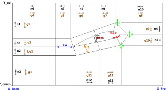
The geometry consists of a 2D airfoil created by a FORTRAN code. The airfoil coordinates are specified in an input file calledAirf oil.data. The mesh parameters can be selected in theinput.data

file. For running the FORTRAN code, you need to open a terminal and go to the directory of it, then type make to compile and finally type ./Airfoil. TheblockMeshDict file is generated and we can use it on OpenFoam to produce our geometry. All relevant parameters are shown in figure (1.1).

(3)

Figure 1.1: Geometry parameters.

1.3 Pre-processing

In this section, we describe the required setting up for four different cases which will be described later.

1.3.1 Getting Started

Copy the simpleFoam tutorial to the run directory.

cp -r $FOAM_TUTORIALS/incompressible/simpleFoam/airFoil2D $FOAM_RUN

cd $FOAM_RUN

The airfoil2D directory consists of different directories such as 0, constant, system where the required settings are done. Since we use different airfoil compared to the OpenFOAM tutorial, we need to remove all files in the /constant/polyMesh and put the blocMeshDict file generated by FORTRAN code on it. Running the BlockMesh command (when we are in the case directory) creates the geometry.

1.3.2 Mesh Generation

After running the FORTRAN code which creates the blockMeshDict file, we must modify the

blockMeshDict file since we would like to divide the computational domain into the two parts (laminar and turbulent), . The only changes we need to make on the blockMeshDict is to add the wordlaminarandturbulentto theblockspart as below. In the blockMeshDict file, vertices section, the order of the mesh points has been specified. Referring to the figure (1.1), the laminar and turbulent blocks are obvious.

(4)

blocks (

hex ( 20 21 29 28 54 55 63 62) turbulent (60 30 1) simpleGrading ( 0.05 25.00 1) hex ( 21 22 30 29 55 56 64 63) turbulent (25 30 1) simpleGrading ( 0.30 25.00 1) hex ( 22 25 31 30 56 59 65 64) turbulent (30 30 1) simpleGrading ( 4.00 25.00 1) hex ( 25 26 32 31 59 60 66 65) laminar (30 30 1) simpleGrading ( 0.20 25.00 1) hex ( 26 27 33 32 60 61 67 66) laminar (50 30 1) simpleGrading (15.00 25.00 1) hex ( 18 19 27 26 52 53 61 60) laminar (50 30 1) simpleGrading (15.00 3.00 1) hex ( 10 11 19 18 44 45 53 52) laminar (50 40 1) simpleGrading (15.00 0.40 1) hex ( 4 5 11 10 38 39 45 44) laminar (50 30 1) simpleGrading (15.00 0.03 1) hex ( 3 4 10 9 37 38 44 43) laminar (25 30 1) simpleGrading ( 0.20 0.03 1) hex ( 2 3 9 8 36 37 43 42) turbulent (25 30 1) simpleGrading ( 3.00 0.03 1) hex ( 1 2 8 7 35 36 42 41) turbulent (25 30 1) simpleGrading ( 0.30 0.03 1) hex ( 0 1 7 6 34 35 41 40) turbulent (60 30 1) simpleGrading ( 0.05 0.03 1) hex ( 6 7 13 12 40 41 47 46) turbulent (60 35 1) simpleGrading ( 0.05 0.10 1) hex ( 12 13 21 20 46 47 55 54) turbulent (60 35 1) simpleGrading ( 0.05 10.00 1) hex ( 13 14 22 21 47 48 56 55) turbulent (25 35 1) simpleGrading ( 0.30 10.00 1) hex ( 14 23 25 22 48 57 59 56) turbulent (30 35 1) simpleGrading ( 4.00 10.00 1) hex ( 23 24 26 25 57 58 60 59) laminar (30 35 1) simpleGrading ( 0.20 10.00 1) hex ( 17 18 26 24 51 52 60 58) laminar (35 30 1) simpleGrading (10.00 3.00 1) hex ( 16 10 18 17 50 44 52 51) laminar (35 40 1) simpleGrading (10.00 0.40 1) hex ( 9 10 16 15 43 44 50 49) laminar (25 35 1) simpleGrading ( 0.20 0.10 1) hex ( 8 9 15 14 42 43 49 48) turbulent (25 35 1) simpleGrading ( 3.00 0.10 1) hex ( 7 8 14 13 41 42 48 47) turbulent (25 35 1) simpleGrading ( 0.30 0.10 1) );

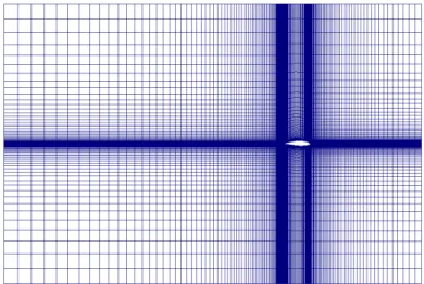
Now, we can runblockMeshto generate the mesh. Since we have determined the laminar and tur-bulent zones at theblockspart of theblockMeshDictfile as above, the mesh will have two different zones as figure (1.2). When we runblockMesh, it creates additional files in thepolyMeshdirectory

Figure 1.2: The laminar (black) and turbulent (white) zones.

ascellZonescomprisinglaminarandturbulentcell labels as well as an additional directory inside thepolymeshdirectory namedsetscomprisinglaminarandturbulentfiles defining cell numbers.

(5)

Figure 1.3: Generated mesh by blockMeshDict.

(6)

1.3.3 Boundary and initial conditions

Since our case is different to the standard OpenFOAM tutorial for airfoil2D, the boundary and initial conditions are changed as below. After running the blockMeshDict, the generated mesh consists of five parts which areinlet,outlet,top, bottomand wing. The free stream velocity and angle of attack are set to 75[m/s] and 5 degree, respectively. The pressure field is considered as relative freestream pressure, equal to zero. Since our turbulence model isSpalartAllmarasmodel and the solver issimpleFoam, we also need to defineνtand ˜νas initial conditions, similar to the value of the OpenFOAM tutorial. The freestream BC has the type inlet/outlet meaning that it looks locally (for every face of the patch) at the mass flow rate. If the flow is going outside the boundary will be locally zero gradient, if it is going inside the boundary will be locally fixedValue. The freestreampressure BC is a zeroGradient BC but it fixes the flux on the boundary.

Velocity dimensions [0 1 -1 0 0 0 0]; internalField uniform (-74.71 6.53 0); boundaryField { inlet { type freestream; freestreamValue uniform (-74.71 6.53 0); } outlet { type freestream; freestreamValue uniform (-74.71 6.53 0); } top { type freestream; freestreamValue uniform (-74.71 6.53 0); } bottom { type freestream; freestreamValue uniform (-74.71 6.53 0); } wing { type fixedValue; value uniform (0 0 0); } defaultFaces { type empty; }

(7)

Pressure dimensions [0 2 -2 0 0 0 0]; internalField uniform 0; boundaryField { inlet { type freestreamPressure; } outlet { type freestreamPressure; } top { type freestreamPressure; } bottom { type freestreamPressure; } wing { type zeroGradient; } defaultFaces { type empty; } } nut dimensions [0 2 -1 0 0 0 0]; internalField uniform 0.14; boundaryField { inlet { type freestream; freestreamValue uniform 0.14; }

(8)

outlet { type freestream; freestreamValue uniform 0.14; } bottom { type freestream; freestreamValue uniform 0.14; } top { type freestream; freestreamValue uniform 0.14; } wing { type nutSpalartAllmarasWallFunction; value uniform 0; } defaultFaces { type empty; } } nuTilda dimensions [0 2 -1 0 0 0 0]; internalField uniform 0.14; boundaryField { inlet { type freestream; freestreamValue uniform 0.14; } outlet { type freestream; freestreamValue uniform 0.14; } bottom { type freestream; freestreamValue uniform 0.14;

(9)

top { type freestream; freestreamValue uniform 0.14; } wing { type nutSpalartAllmarasWallFunction; value uniform 0; } defaultFaces { type empty; } }

1.3.4 Constant

In theconstantdirectory, we need to modifyRASPropertiesrelevant to our turbulence model. So, the originalRASProperties

RASModel SpalartAllmaras;

turbulence on;

printCoeffs on;

must be changed based on theRASModel. Since we are going to define four different turbulence model, then theRASModelmust be different for each case. Below is one example of theRASPropertiesfile:

RASModel mySpalartAllmaras;

turbulence on;

printCoeffs on;

1.3.5 System

To define the laminar and turbulent zones, we use two different approaches. The first approach is to use the color function (alpha1=0/1) and the other one is to use cellZone class which will be explained later. For the first approach, we need to copy the below command

cp -r $WM_PROJECT_DIR/tutorials/multiphase/interFoam/laminar/damBreak/system/setFieldsDict .

to thesystemdirectory of our case.

1.3.6 setFieldsDict

SetFieldsDict dictionary, located in the system directory, is a utility file which specifies a non-uniform initial condition. The originalsetFieldsDictfile reads as

defaultFieldValues (

(10)

); regions ( boxToCell { box (0 0 -1) (0.1461 0.292 1); fieldValues ( volScalarFieldValue alpha1 1 ); } );

We change the originalsetFieldsDictas below:

defaultFieldValues ( volScalarFieldValue alpha1 1 ); regions ( zoneToCell { name laminar; fieldValues ( volScalarFieldValue alpha1 0 ); } );

We definevolScalarFieldValue alpha1equal to1for the whole domain by

defaultFieldValues (

volScalarFieldValue alpha1 1 );

then we modify it its value tozerofor the laminar zone by

regions ( zoneToCell { name laminar; fieldValues ( volScalarFieldValue alpha1 0 ); } );

Please note that we only need thesetFieldsDictfile in thesystemdirectory for the case based on the color function.

(11)

ThecontrolDictdictionary sets input parameters essential for the creation of the database. In the

controlDict file, we need to modify some parameters related to our solution. Below, you can see thecontrolDictfile. The ”lib (”libmyIncompressibleRASModels.so”);” term is described later.

application simpleFoam; startFrom latestTime; startTime 0; stopAt endTime; endTime 2000; deltaT 0.5; writeControl timeStep; writeInterval 400; purgeWrite 0; writeFormat ascii; writePrecision 6; writeCompression uncompressed; timeFormat general; timePrecision 6; runTimeModifiable yes; libs ("libmyIncompressibleRASModels.so"); functions { forces { type forceCoeffs; functionObjectLibs ( "libforces.so" ); outputControl timeStep; outputInterval 1; patches ( wing ); pName p; UName U; rhoName rhoInf; log true; rhoInf 1; CofR ( 0 0 0 );

(12)

liftDir ( 0.087 0.996 0 ); dragDir ( -0.996 0.087 0 ); pitchAxis ( 0 0 1 ); magUInf 75.00; lRef 1; Aref 1; } }

1.4 Modified Turbulence Model

As mentioned before, we are interested to investigate the flow transition from laminar to turbulence on the airfoil. We can do it in four different ways.

1. Using color function (alpha1=0/1) for defining the laminar and turbulent zone and setting

νt= 0 (turbulent viscosity) for laminar zone.(mySpalartAllmaras case)

2. UsingcellZoneclass to distinct the laminar and turbulent zone and settingνt= 0 (turbulent viscosity) for laminar zone.(myZoneSpalartAllmaras)

3. Using color function (alpha1=0/1) for defining the laminar and turbulent zone and setting the

Pk_{= 0 (production term in ˜}_ν _{equation) for laminar zone.(myAlphaPdcSpalartAllmaras)} 4. Using cellZone class to distinct the laminar and turbulent zone and setting the Pk _{= 0}

(production term in ˜ν equation) for laminar zone.(myPdcSpalartAllmaras)

The turbulence model which is used in this tutorial is Spalart-Allmaras one-equation model with

fv3 term. It is defined as (http://turbmodels.larc.nasa.gov/spalart.html)

∂ν˜ ∂t +uj ∂ν˜ ∂xj =Cb1[1−ft2] ˜Sν˜+ 1 σ{∇ ·[(ν+ ˜ν)∇˜ν] +Cb2|∇ν| 2_{} −} Cw1fw− Cb1 κ2 ft2 ˜ ν d 2 +ft1∆U2 (1.1) with the following exceptions:

˜ S≡fv3Ω + ˜ ν κ2_d2fv2, fv2= 1 1 + χ cv2 3, fv3= (1 +χfv1) (1−fv2) χ , cv2= 5 (1.2)

For implementation of our own turbulence model, we need to copy the source of the turbulence model which we want to use. Here, we will create our own copy of the mySpalartAllmaras turbulence model.

cd $WM_PROJECT_DIR

cp -r --parents src/turbulenceModels/incompressible/RAS/SpalartAllmaras $WM_PROJECT_USER_DIR cd $WM_PROJECT_USER_DIR/src/turbulenceModels/incompressible/RAS/SpalartAllmaras

mv SpalartAllmaras mySpalartAllmaras cd mySpalartAllmaras

Since we need to modify our turbulence model in four different ways, we need to create four fold-ers in the mySpalartAllmaras folder. Those are mySpalartAllmaras, myZoneSpalartAllmaras,

myAlphaPdcSpalartAllmarasandmyPdcSpalartAllmaras. We also need Make/filesandMake/options. Create aMake directory:

mkdir Make

(13)

myZoneSpalartAllmaras/myZoneSpalartAllmaras.C

myAlphaPdcSpalartAllmaras/myAlphaPdcSpalartAllmaras.C myPdcSpalartAllmaras/myPdcSpalartAllmaras.C

LIB = $(FOAM_USER_LIBBIN)/libmyIncompressibleRASModels

Create/Make/optionsand add:

EXE_INC = \ -I$(LIB_SRC)/turbulenceModels \ -I$(LIB_SRC)/transportModels \ -I$(LIB_SRC)/finiteVolume/lnInclude \ -I$(LIB_SRC)/meshTools/lnInclude \ -I$(LIB_SRC)/turbulenceModels/incompressible/RAS/lnInclude LIB_LIBS =

(the last -I is needed since mySpalartAllmaras uses include-files in the original directory). We need to modify the file names of our new turbulence models.

rename SpalartAllmaras mySpalartAllmaras *

InmySpalartAllmaras.C,mySpalartAllmaras.H,myZoneSpalartAllmaras.Cand

myZoneSpalartAllmaras.H,myAlphaPdcSpalartAllmaras.C,myAlphaPdcSpalartAllmaras.H,

myPdcSpalartAllmaras.CandmyPdcSpalartAllmaras.H, we must change all occurances of Spalar-tAllmaras tomySpalartAllmaras,myZoneSpalartAllmaras,myAlphaPdcSpalartAllmarasand

myPdcSpalartAllmaras. So, we have four new classes name:

sed -i s/SpalartAllmaras/mySpalartAllmaras/g mySpalartAllmaras.C sed -i s/SpalartAllmaras/mySpalartAllmaras/g mySpalartAllmaras.H

sed -i s/SpalartAllmaras/myZoneSpalartAllmaras/g myZoneSpalartAllmaras.C sed -i s/SpalartAllmaras/myZoneSpalartAllmaras/g myZoneSpalartAllmaras.H

sed -i s/SpalartAllmaras/myAlphaPdcSpalartAllmaras/g myAlphaPdcSpalartAllmaras.C sed -i s/SpalartAllmaras/myAlphaPdcSpalartAllmaras/g myAlphaPdcSpalartAllmaras.H

sed -i s/SpalartAllmaras/myPdcSpalartAllmaras/g myPdcSpalartAllmaras.C sed -i s/SpalartAllmaras/myPdcSpalartAllmaras/g myPdcSpalartAllmaras.H

We can add the below line within the curly brackets of the constructor inmySpalartAllmaras.Cto ensure that our model is working.

Info << "Defining my own SpalartAllmaras model" << endl;

After the above changes, we must compile our new turbulence model:

wclean lib wmake libso

which will build a dynamic library. Finally, we must include our new library by adding a line to/system/controlDict:

libs ("libmyIncompressibleRASModels.so");

It is recommended to use wclean lib instead of wclean, since the wclean lib also cleans the

(14)

In our case, the turbulence model for the simpleFoam solver is SpalartAllmaras model. In order to use it for our cases which have been divided into the laminar and turbulent parts, we need to modify it. The idea which we applied for distinction of laminar and turbulent flow in our solution is based on the turbulent viscosity definition and turbulent production term. TheSpalartAllmaras

turbulence model is a one equation model solving a transport equation for a viscosity-like variable ˜ν. In the first approach, Sinceνt= ˜νfv1(whereνtandfv1denote turbulent viscosity and a coefficient,

respectively), we can say that for the laminar flow, νt = 0 and for turbulent flow, it is not zero. Therefore, we multiplyalpha1_.internalField()in the\nu_tequation in theConstructorspart of themySpalartAllmaras.C. In the second approach, we only set the turbulent production term,

Pk = 0, in the ˜ν equation for laminar zone.

In the$WM_PROJECT_USER_DIR/src/turbulenceModels/incompressible/RAS/mySpalartAllmaras

directory, we find four folders,mySpalartAllmaras,myZoneSpalartAllmaras,myAlphaPdcSpalartAllmaras

andmyPdcSpalartAllmaras. The color function (alpha1 = 0/1) is used in themySpalartAllmaras

andmyAlphaPdcSpalartAllmarasdirectory to distinct the laminar and turbulent zone while in the other approaches (myZoneSpalartAllmarasandmyPdcSpalartAllmarasdirectory) cellZone con-struction is used.

1.4.1 mySpalartAllmaras

In this directory, we have three files:

mySpalartAllmaras.C mySpalartAllmaras.dep mySpalartAllmaras.H

Since we use color function (alpha1=0for laminar zone andalpha1=1for turbulent zone), we need to define it. So, thealpha1_must be added into theConstructorssection of themySpalartAllmaras.C. So, we will have

nuTilda_ ( IOobject ( "nuTilda", runTime_.timeName(), mesh_, IOobject::MUST_READ, IOobject::AUTO_WRITE ), mesh_ ), alpha1_ ( IOobject ( "alpha1", runTime_.timeName(), mesh_, IOobject::MUST_READ, IOobject::AUTO_WRITE ), mesh_ ),

(15)

( IOobject ( "nut", runTime_.timeName(), mesh_, IOobject::MUST_READ, IOobject::AUTO_WRITE ), mesh_ ),

Please note that the orders of thenuTilda_, alpha1_andnut_in theConstructorssection of the

mySpalartAllmaras.Cmust be the same as their order in themySpalartAllmaras.Hfile, otherwise we will receivewarningduring compile of turbulence model. Also, we need to definealpha1_in the

mySpalartAllmaras.Hfile for declaration. Therefore, we modify the following items as

// Fields volScalarField nuTilda_; volScalarField alpha1_; volScalarField nut_; wallDist d_; and // Member Functions

//- Return the turbulence viscosity virtual tmp<volScalarField> nut() const {

return nut_; }

virtual tmp<volScalarField> alpha1() const {

return alpha1_; }

1.4.2 myZoneSpalartAllmaras

myZoneSpalartAllmaras.C myZoneSpalartAllmaras.dep myZoneSpalartAllmaras.H

Here, we do not use color function (alpha = 0/1). So, we need to find a way in which the tur-bulence model be capable to access the cell zones of the grid in order to use a suitable νt for distinction between the laminar and turbulent zones. The following lines must be added into the

Member Functionssection of themyZoneSpalartAllmaras.Cafter the definition ofnutilda_.internalField(), so we will have

(16)

forAll(mesh_.cellZones(), i) {

const cellZone& zone = mesh_.cellZones()[i];

if (zone.name()=="laminar") {

const labelList& cellLabels = mesh_.cellZones()[i];

Info<< " Found matching zone " << zone.name()

<< " with " << cellLabels.size() << " cells." << endl;

forAll(cellLabels, i) { nut_.internalField()[cellLabels[i]]=0.0; } } }

The above code can be applied in another way as below:

Info<< " Found matching zone " << zone.name() << " with " << zone.size() << " cells." << endl;

forAll(zone, i) {

nut_.internalField()[zone[i]]=0.0;

Info<<"We are in zone"<<zone.name()<<"and cell"<<i<<endl;

} } }

The possibility for doing this method is that thezonein thecellZone& zone = mesh_.cellZones()[i];

is an object of the classcellZone. Since thecellZoneis a list, then it can call functions that belongs to the list.

1.4.3 myAlphaPdcSpalartAllmaras

myAlphaPdcSpalartAllmaras.C myAlphaPdcSpalartAllmaras.dep myAlphaPdcSpalartAllmaras.H

Here , again we use color function (alpha=0/1) to define the laminar and turbulent region. Our turbulence model , SpalartAllmaras, solves the ˜ν equation. The production term in the ˜ν eqation

(17)

following codes show how we implement this method by using color function where alpha1 = 0 for laminar region and alpha1 = 1 for turbulent region. Please note that in this model, we also need to define alpha1 again in the same way as we did for mySpalartAllmaras model. In the

$WM_PROJECT_USER_DIR/src/turbulenceModels/incompressible/RAS/mySpalartAllmaras \ myAlphaPdcSpalartAllmarasdirectory, we modify the ˜ν eqation as below:

tmp<fvScalarMatrix> nuTildaEqn ( fvm::ddt(nuTilda_) + fvm::div(phi_, nuTilda_) - fvm::Sp(fvc::div(phi_), nuTilda_) - fvm::laplacian(DnuTildaEff(), nuTilda_) - Cb2_/sigmaNut_*magSqr(fvc::grad(nuTilda_)) == alpha1_*Cb1_*Stilda*nuTilda_ - fvm::Sp(Cw1_*fw(Stilda)*nuTilda_/sqr(d_), nuTilda_) );

1.4.4 myPdcSpalartAllmaras

myPdcSpalartAllmaras.C myPdcSpalartAllmaras.dep myPdcSpalartAllmaras.H

In this method, instead of using color function, we use thecellZonesclass to distinct between the laminar and turbulent zones. For the laminar flow, we set the production term in the ˜ν eqation (Pk =Cb1˜s˜ν) equal to zero whereas it is not zero for turbulent region.The following lines must be

added into the Member Functions section of the myPdcSpalartAllmaras.C after the definition of

volScalarField Stilda, so we will have

Info<< " Found matching zone " << zone.name() << " with " << zone.size() << " cells." << endl;

tmp<fvScalarMatrix> nuTildaEqn ( fvm::ddt(nuTilda_) + fvm::div(phi_, nuTilda_) - fvm::Sp(fvc::div(phi_), nuTilda_) - fvm::laplacian(DnuTildaEff(), nuTilda_) - Cb2_/sigmaNut_*magSqr(fvc::grad(nuTilda_)) == - fvm::Sp(Cw1_*fw(Stilda)*nuTilda_/sqr(d_), nuTilda_) ); nuTildaEqn().relax();

(18)

solve(nuTildaEqn);

bound(nuTilda_, dimensionedScalar("0", nuTilda_.dimensions(), 0.0)); nuTilda_.correctBoundaryConditions(); nut_.internalField() = fv1*nuTilda_.internalField(); nut_.correctBoundaryConditions(); } else { tmp<fvScalarMatrix> nuTildaEqn ( fvm::ddt(nuTilda_) + fvm::div(phi_, nuTilda_) - fvm::Sp(fvc::div(phi_), nuTilda_) - fvm::laplacian(DnuTildaEff(), nuTilda_) - Cb2_/sigmaNut_*magSqr(fvc::grad(nuTilda_)) == Cb1_*Stilda*nuTilda_ - fvm::Sp(Cw1_*fw(Stilda)*nuTilda_/sqr(d_), nuTilda_) ); nuTildaEqn().relax(); solve(nuTildaEqn);

bound(nuTilda_, dimensionedScalar("0", nuTilda_.dimensions(), 0.0)); nuTilda_.correctBoundaryConditions();

nut_.internalField() = fv1*nuTilda_.internalField();

nut_.correctBoundaryConditions();

}

1.5 Lift and Drag Forces Coefficient

In order to compute the lift and drag coefficients, we can useforceCoeffs functionObject. The

functionObjectsare general libraries that can be attached run-time to any solver, without having to re-compile the solver. TheforceCoeffs functionObjectis available on thesonicFoamsolver. We need to add the below part to thesystem/controlDict and modify the values relevant to our case. In this function, the liftDir and dragDir are defined based on the angle of attack. The

magUInfdenotes the magnitude of the freestream velocity. Please note that since the dimension of the pressure in the compressible flow has been set different to the dimension of the pressure in the incompressible flow, we need to definerhoNameasrhoInf. Therefore, we have

functions {

forces {

(19)

functionObjectLibs ( "libforces.so" ); outputControl timeStep; outputInterval 1; patches ( wing ); pName p; UName U; rhoName rhoInf; log true; rhoInf 1; CofR ( 0 0 0 ); liftDir ( 0.087 0.996 0 ); dragDir ( -0.996 0.087 0 ); pitchAxis ( 0 0 1 ); magUInf 75.00; lRef 1; Aref 1; } }

By adding the forceCoeffs functionObject into the system/controlDict, while running the case, a new directory namedforcesis created in the case directory writing theCL andCD in each run time.

1.5.1 Running the code

Now, we can run our cases as below. We have four different cases,

my_airfoil_alpha1_pdc my_airfoil_alpha1 my_airfoil_zone_pdc my_airfoil_zone

Therefore, for running the first case, we can do as below and for other cases we can do the same.

cd $FOAM_RUN/my_airfoil_alpha1 simpleFoam

1.6 Post-processing

When the case running is finished, we can see our results by using the paraView software as

cd $FOAM_RUN/my_airfoil_alpha1 paraFoam

Here are the results of four different transient cases compared to the non-transient case. 1. mySpalartAllmaras

2. myZoneSpalartAllmaras 3. myAlphaPdcSpalartAllmaras 4. myPdcSpalartAllmaras 5. Standard case (no transition)

(20)

Figure 1.5: Case No.1, Pressure field around the airfoil

(21)

Figure 1.7: Case No.1, Turbulent viscosity field around the airfoil

(22)

Figure 1.9: Case No.2, Velocity field around the airfoil

(23)

Figure 1.11: Case No.3, Pressure field around the airfoil

(24)

Figure 1.13: Case No.3, Turbulent viscosity field around the airfoil

(25)

Figure 1.15: Case No.4, Velocity field around the airfoil

(26)

Figure 1.17: Standard case, Pressure field around the airfoil

(27)

Figure 1.19: Standard case, Turbulent viscosity field around the airfoil

The computed lift and drag coefficients for different cases are shown below: Case Cl Cd 1 0.1117 0.0013 2 0.1117 0.0013 3 0.1005 0.0029 4 0.1005 0.0029 Standard 0.1003 0.0030