Supporting a Light-Weight Data Management Layer Over HDF5

Supporting a Light-Weight Data Management Layer

Over HDF5

Yi Wang Yu Su Gagan Agrawal

Department of Computer Science and Engineering The Ohio State University Columbus OH 43210

{wayi,su1,agrawal}@cse.ohio-state.edu Abstract—Scientific simulations are now being performed at finer

temporal and spatial scales, leading to an explosion of the output data, and challenges in storing, managing, disseminating, analyzing, and visualizing these datasets. Tools commonly used today for disseminating and visualizing such data have inherent limitations, making it extremely hard to deal with larger datasets.

We have developed a light-weight data management tool, which allows server-side subsetting and aggregation on scientific datasets stored in HDF5, one of the most popular scientific data formats. To support a variety of queries efficiently, our tool generates code for hyperslab selector and content-based filtering, and parallelizes selection and aggregation queries efficiently using novel algorithms. Additionally, our tool also supports certain most recent HDF5 features including dimension scale and compound datatype.

Through extensive evaluation, we show that our system is capable of efficiently supporting a variety of queries, scaling performance by parallelizing the queries, and reducing wide area data transfers through server-side data aggregation. We demonstrate that even for subsetting queries that are directly supported in OPeNDAP, a tool widely used by data dissemination portals, the sequential performance of our system is better.

I. INTRODUCTION

Many of the ‘big-data’ challenges today are arising from in-creasing computing ability, as data collected from simulations has become extremely valuable for a variety of scientific endeavors. With growing computational capabilities of parallel machines, scientific simulations are being performed at finer spatial and temporal scales, leading to data explosion.

Finer granularity of simulation data offers both an opportunity and a challenge. On one hand, it can allow understanding of underlying phenomenon and features in a way that would not be possible with coarser granularity. On the other hand, larger datasets are extremely difficult to store, manage, disseminate, analyze, and visualize. Neither the memory capacity of paral-lel machines, memory access speeds, nor disk bandwidths are increasing at the same rate as computing power, contributing to the difficulty in storing, managing, and analyzing these datasets. Simulation data is often disseminated widely, through portals like the Earth System Grid (ESG), and downloaded by researchers all over the world. Such dissemination efforts are hampered by dataset size growth, as wide area data transfer bandwidths are growing at a much slower pace. Finally, while visualizing datasets, human perception is inherently limited.

In the context of visualization, for almost all simulations, the dataset sizes have grown well past the point that it is infeasible for a scientist to look through all of the data [12]. In addition, because of growing dataset sizes, most of the time while performing data visualization and analysis is now spent in I/O routines, reducing the effectiveness of a visualization effort.

Despite much emphasis on large-scale visualization, the state-of-the-art in dealing with large-scale datasets is very limited. If we look at the current popular tools, like ParaView and VisIt, most subsetting operations are done through an in-memory interface, where all data is loaded at once. Then, either throughfiltering, i.e.,

applying data transformations, orselectioninterfaces, the data is subset. The memory footprint for this operation is the total size of the data plus the size of the data after subsetting operations. Clearly, with growing dataset sizes, this is a serious limitation. Therefore, we must look towards pushing data subsetting and querying operations in large-scale analysis tools to the I/O level (i.e. perform them prior to loading all the data in memory), to cope with the memory limitations. Similarly, while disseminating data, in many of the existing data dissemination portals (e.g., Earth System Grid (ESG)) data downloading is facilitated by OPeNDAP [8], which has only a very limited support for data subsetting, and no support for aggregation at the server side.

The key underlying reason for the limited state-of-the-art is that the management of scientific (array-based) data has received very limited attention over years. On one hand, while a typical database provides a high-level query language, it also requires all data to be loaded into the system, which is often extremely time-consuming. On the other hand, more ad-hoc solutions for data management, which do not require that data be reloaded in such a fashion, unfortunately involve format-specific coding and use of lower-level languages.

In this paper, we describe an approach which involves the best of both of the two approaches. On one hand, our approach does not require data to be loaded into a specific system or be reformatted. At the same time, we allow use of a high-level language for specification of processing, which is also independent of the data format. We present an implementation of this approach for HDF5, one of the most popular formats for storing scientific data. (The following documentation lists some of the major users of HDF51_{.) Our tool supports SQL select and}

aggregation queries specified over thevirtual relational table view of the data. Besides supporting selection overdimensions, which is directly supported by HDF5 API also, we also support queries involvingdimension scalesand those involvingdata values. For this, we generate code forhyperslab selectorandcontent-based filterin our system. We also effectively parallelize selection and aggregation queries using novel algorithms.

We have extensively evaluated our implementation with queries of different types, and have compared its performance and functionality against OPeNDAP. We demonstrate that even for subsetting queries that are directly supported in OPeNDAP, the sequential performance of our system is better by at least a factor of 3.9. For other types of queries, where OPeNDAP requires hyperslab selector and/or content-based filter code to be written manually, the performance difference is even larger. In addition, our system is capable of scaling performance by parallelizing the queries, and reducing wide area data transfers through server-side data aggregation. In terms of functionality, our system also supports certain state-of-the-art HDF5 features including dimension scale and compound datatype.

1_{http://www.hdfgroup.org/HDF5/users5.html}

II. BACKGROUND

This section provides background information on HDF5 data format and its high-level libraries.

A. HDF5

HDF5 [1] is a widely used data model, library, and file format for storing and managing data. It supports a variety of data types, and is designed for flexible and efficient I/O and for high volume and complex data. HDF5 is portable and extensible, and HDF5 files are organized in a hierarchical structure, with two primary structures: groups and datasets. A group contains instances of zero or more groups or datasets, and a dataset is essentially a multidimensional array of data elements, where both of them can have associated metadata.

Additionally, HDF5 is designed to support any data type, so, besides a limited number of atomic datatypes,compound datatype is also supported in HDF5. A compound datatype may have an arbitrary number of data members in any order, and the data members may be of any datatype, including compound. B. High-Level HDF5

The HDF5 high-level APIs [2] provide a set of functions built on top of the basic HDF5 Library. The purpose of the high-level API is two-fold: 1) to define functions that perform more complex operations in a single call, as compared to the basic HDF5 interface, and 2) to build sets of functions that provide standard entity definitions (like images or tables).

HDF5dimension scaleis one of important features here. An HDF5 dimension scale is an auxiliary dataset that is associated with a dimension of a primary dataset. It can serve as a coordinate system support for the primary dataset by constructing a mapping between values of dimension index and values of the dimensional scale dataset. A common example is a 2-dimensional array with spatial information, such as latitude and longitude, associated with it.

III. SYSTEMDESIGN

In this section, we discuss the design and implementation of our system.

A. Motivation

HDF5 dataset is stored in binary format. The advantage is that it supports self-describing, portable, and compact storage, as well as efficient I/O. At the same time, the disadvantage is that the API involves overly nitty-gritty details which make the data processing much harder, forcing scientists who are interested in data subsetting to have a very detailed understanding of the data layout before being able to extract the subset. In addition, they also have to get familiar with the HDF5 libraries in order to write an application that can extract the subset. For each different subsetting task, the scientists may need to write a separate program.

To address these problems, our solution involves three ideas. The first idea is that a virtual relational table view can be supported over HDF5 dataset, and standard SQL queries with SELECT,FROM, andWHEREclauses on such a view can provide a very convenient yet powerful way to specify the data subsetting. The second idea is that data aggregation and group-by, using the same abstractions, can be applied to extract data summaries, which can minimize data transfer costs. The third idea is that sequential subsetting of data can be prohibitively expensive with growing datasets, and therefore, it’s more desirable to exploit parallelism to accelerate data subsetting and aggregation queries. An HDF5 dataset consists of a set of multi-dimensional arrays. These arrays typically involve spatial and/or temporal dimensions and, in many cases, corresponding dimension scales as well. Scientists are usually interested in querying a subset of the data based on the either dimension indices or coordinate system

expressed by dimension scales. Hence, we can divide the queries into three categories: 1) Queries based on dimensional index value(s) - i.e. those related with the dataset physical layout; 2) Queries based on coordinate value(s) - Besides the dimension information, the scientists may also query data subsets based on spatial or temporal values, which are usually stored in dimension scales; 3) Queries based on data value(s) - The scientists could also query the target data value within a specific value range.

Similarly, we can also categorize all the query conditions into three types: index-based, coordinate-based, and content-based conditions. The goal of our system is to support any combination of the above three types of queries.

B. System Overview

Figure 1 gives an overview of the execution flow of processing a typical query using our system. The purpose of our system is to translate an SQL query into efficient data access code in HDF5 context and to complete the query by parallel access. After an SQL query passes through an SQL parser, the SQL parser extracts all the paths (from the FROM clause) of HDF5 files involved in that query, and then it sends this information to a metadata generator. Afterwards, the metadata generator accesses to all the required HDF5 files according to the paths retrieved by the SQL parser, and then it generates metadata at runtime. The detailed information about the metadata and the metadata generation strategy will be introduced in Section IV.

The SQL parser is used to generate a 2-dimensional query list. First, all the elementary queries in the sameANDclause will be organized in the same 1-dimensional query list. Second, all these 1-dimensional lists will be grouped in an OR-logic and hence organized in a 2-dimensional list. Our parser is implemented with certain modifications of the parser from SQLite [4].

64/ 4XHU\ 64/ 3DUVHU +') )LOHV '4XHU\ /LVW 0HWDGDWD *HQHUDWRU ,Q6LWX 0HWDGDWD +\SHUVODE 6HOHFWRU '4XHU\ /LVW 4XHU\ 3URFHVVRU &RQWHQW%DVHG )LOWHU

/RFDO 4XHU\ 5HVXOW

4XHU\ 3DUWLWLRQ

6XETXHU\

/RFDO 4XHU\ 5HVXOW /RFDO 4XHU\ 5HVXOW

4XHU\ &RPELQDWLRQ

*OREDO 4XHU\ 5HVXOW

6XETXHU\ 6XETXHU\ 6XETXHU\

Fig. 1. Execution Overview

The hyperslab selector module mainly performs three tasks: First, for all the coordinate values that appear in the queries, convert them into index values specific to the physical layout, by retrieving corresponding dimension scales from the metadata. Second, for each 1-dimensional query list organized in an AND-logic, combine all the elementary queries into a single compos-ite (and probably reduced) query. Third, with the data layout information provided by the metadata and the index value(s) provided in the query condition, each composite query can

generate a hyperslab on the hyperspace. As a result, a collection of hyperslabs are selected, and a final 1-dimensional query list is generated. The detailed information about the hyperslab selector will be discussed in Section V.

The query partition module is used to divide each query in the 1-dimensional query list into multiple subqueries. Each subquery is a query with the same content-based condition as the one in the original query, yet responsible for a disjoint subset of the original hyperslab. Thus, each process executes one subquery, and hence collective I/O can be used to achieve better performance compared with independent I/O. The detailed information about the query partition will be discussed in Section V.

With the hyperslab information generated during the previous phases, the query processor is used to invoke native HDF5 calls to perform data accesses. After query processing, each subquery retrieves the required data block, but all the content-based conditions, which are dependent on data values, still remain to be checked. Content-based filter then performs a full scan over the data block retrieved after query processing, to filter out the data elements which cannot satisfy the condition. However, since aggregation query also requires the same full scan, content-based filtering actually can be performed while processing aggregation queries. In this way, there will be always one full scan at most during the entire execution flow.

Finally, each process obtains a local query result. For aggrega-tion queries, a query combinaaggrega-tion is needed to generate the global query result. For non-aggregation queries, the combination is considerably expensive because it requires massive data transfer. Fortunately, most applications only require each process to output all local results in a specified order.

IV. METADATAGENERATIONSTRATEGY

In this section, we discuss the design and implementation of the metadata generation strategy.

For each input query, ametadata generatoris used to collect metadata at runtime, without requiring a loading process before-hand. The function of the metadata generator is to collect dataset physical storage information, datasetlogical layout information, and user metadata (i.e. intrinsic header metadata) stored in the header. The motivation for this design is three-fold: First, a large HDF5 dataset may be distributed among multiple files. Query processing requires dataset physical storage information from each of these files, and therefore, it is desirable to collect this information at one place. Second, certain dataset logical layout

information such as dataset dimensions and dimension scales

is often frequently required during query processing. Again, prefetching this information in advance is desirable, so we can avoid repeated I/O requests during query processing. Third, HDF5 datasets are organized in a hierarchical structure, so the user metadata may be dispersed in separate header blocks for each object. Therefore, collecting the scattered user metadata can also help reduce the header I/O overhead.

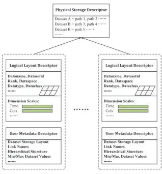
As Figure 2 shows, the metadata structure consists of three components: 1) Physical Storage Descriptor: It describes physical locations where each dataset is resident. All the paths of the required dataset files are specified in the FROM clause in an SQL query, thus by recording the datasets contained in these files, each dataset involved in the query can be mapped to a set of corresponding file paths. 2) Logical Layout Descriptor: It exposes the low-level dataset layouts, including datatypes, dataspaces, and dimension scales. Specifically, dimension scales, which are relatively quite small datasets, are fully loaded to support the queries that are based on coordinate values. 3) User Metadata Descriptor: It contains the descriptions about user metadata, which is optionally defined and provided by the users. Some user-provided information such as minimum/maximum dataset values can facilitate the later processing such like hyperslab selection.

‘‰‹…ƒŽƒ›‘—–‡•…”‹’–‘” 'DWDQDPH 'DWDVHWLG 5DQN 'DWDVSDFH 'DWDW\SH 'DWDFODVV ĂĂ 'LPHQVLRQ 6FDOHV 7LPH &ROV ĂĂ •‡”‡–ƒ†ƒ–ƒ‡•…”‹’–‘” 'DWDVHW 6WRUDJH /D\RXW /LQN 1DPHV +LHUDUFKLFDO 6WXUFWXUH 0LQ0D[ 'DWDVHW 9DOXHV ĂĂ ‘‰‹…ƒŽƒ›‘—–‡•…”‹’–‘” 'DWDQDPH 'DWDVHWLG 5DQN 'DWDVSDFH 'DWDW\SH 'DWDFODVV ĂĂ 'LPHQVLRQ 6FDOHV 7LPH &ROV ĂĂ •‡”‡–ƒ†ƒ–ƒ‡•…”‹’–‘” 'DWDVHW 6WRUDJH /D\RXW /LQN 1DPHV +LHUDUFKLFDO 6WXUFWXUH 0LQ0D[ 'DWDVHW 9DOXHV ĂĂ Š›•‹…ƒŽ–‘”ƒ‰‡‡•…”‹’–‘” 'DWDVHW $ SDWK SDWK ĂĂ 'DWDVHW % SDWK SDWK ĂĂ 'DWDVHW % SDWK ĂĂ ĂĂ

ĂĂ

Fig. 2. Metadata Structure

V. QUERYEXECUTION

In this section, we discuss our query execution methods, including hyperslab selection, content-based filtering, processing of aggregation queries, and parallelization of both selection and aggregation queries.

A. Hyperslab Selection and Content-Based Filtering

Recall that in Section III, we had identified three types of queries, which are queries based on dimensional index values, coordinate values, and data values, respectively. The standard HDF5 API can only support the first type of queries (based on dimensional index values). Even for these queries, one has to know the exact index range, which, in turn, requires a detailed understanding of the data layout. As the high-level HDF5 feature dimension scale becomes increasingly popular in real applica-tions, a growing number of queries involves subsetting on spatial and/or temporal attributes, which are queries based on coordinate values. Currently, for such queries, users have to first query the dimension scales, manually determine each index range based on these values, and then they can perform a subsetting query with the index range. This requires complex programming with detailed knowledge of HDF5 APIs and its programming models, and even the query execution time can be unnecessarily high.

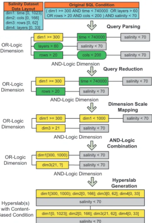
In our system, we use hyperslab selector combined with content-based filterto both improve efficiency and support higher-level operators. Figure 3 shows an example of how the

hyper-slab selector module works. In the example, we queried a

4-dimensional dataset calledsalinity, where 4 dimension scales

time, cols, rows and layersare associated with these 4 dimensions, respectively. In an SQL query, all the target dataset names are required to appear in theSELECTclause, and all the required HDF5 file names have to be specified in the FROM clause.

After the initial query parsing, the SQL parser generates a 2-dimensional query list based on the query condition. As we mentioned earlier in Section III, for a 2-dimensional query list, the lower dimension is an AND-logic dimension, and the higher dimension is an OR-logic dimension. Any original SQL condition can be broken into multiple elementary queries, each of which is organized in this fashion, and each elementary query corresponds to only one condition type. For instance, for the first row in

GLP! WLPH VDOLQLW\

OD\HUV ! VDOLQLW\

2ULJLQDO 64/ &RQGLWLRQ

GLP! $1' WLPH 25 OD\HUV ! 25 URZV ! $1' FROV $1' VDOLQLW\

URZV ! FROV 25/RJLF 'LPHQVLRQ $1'/RJLF 'LPHQVLRQ GLP! WLPH VDOLQLW\ URZV ! VDOLQLW\ 25/RJLF 'LPHQVLRQ $1'/RJLF 'LPHQVLRQ 4XHU\ 5HGXFWLRQ 'LPHQVLRQ 6FDOH 0DSSLQJ GLP! GLP VDOLQLW\ GLP ! VDOLQLW\ 25/RJLF 'LPHQVLRQ $1'/RJLF 'LPHQVLRQ $1'/RJLF &RPELQDWLRQ VDOLQLW\ +\SHUVODE *HQHUDWLRQ GLP> GLP> @ GLP> @ GLP> @ VDOLQLW\ 25/RJLF 'LPHQVLRQ 4XHU\ 3DUVLQJ +\SHUVODEV ZLWK &RQWHQW %DVHG &RQGLWLRQ GLP> @ GLP> @ GLP @ GLP> @ VDOLQLW\ GLP> VDOLQLW\ GLP "@ VDOLQLW\ $1'/RJLF 'LPHQVLRQ GLP WLPH > @ GLP FROV > @ GLP URZV > @ GLP OD\HUV > @ 6DOLQLW\ 'DWDVHW 'DWD /D\RXW

Fig. 3. Hyperslab Selector Module

the query list after query parsing, dim1 refers to the index value of first dimension so thatdim1>=300 is anindex-based condition,time<740000is acoordinate-basedcondition, and

salinity<70is acontent-basedcondition.

In the next step, query reductionis performed to reduce the number of elementary queries. The goal of this phase is to avoid unnecessary or redundant data accesses in the query processing. We perform the query reduction mainly based on the following three query reduction rules: 1) If an elementary query condition is unconditionally false, then the 1-dimensional query list where this query condition belongs can be nullified; 2) If an elementary query condition is unconditionally true, then this single query condition in this dimension can be nullified; and 3) For any two elementary conditions in the same AND-logic dimension, if either query range is entirely covered by the other, then the condition with the larger query range can be nullified. Since all the boundary values of indices and dimension scales have been stored in the metadata, we can apply the above rules without loading the dataset. In the example, since the maximum values oflayers

andcolsare 33 and 166 respectively, the second 1-dimensional query list which containslayers>60can be removed according to the first rule, andcols<200can also be removed from the last 1-dimensional query list because of the second rule. Specifically, the third rule is often applied after the later dimension scale mappingphase. Assume that the query conditiontime<740000

in the first 1-dimensional query list istime>740000 instead, since time is associated with the first dimension, this query condition is equivalent to the index-based conditiondim1>1000. Because this query range is entirely covered by another directly-specified query range dim1>=300 in the same query list, we can nullify the larger query range dim1>=300 based on the third rule. Additionally, since HDF5 library allows one dataset dimension to be associated with multiple dimension scales, a variance of the above case is a query condition involves two different dimension scales which yet correspond to the same dimension. Moreover, besides the boundary values of indices and dimension scales, if the minimum/maximum dataset values are provided in the original user metadata, then we can also apply

the above rules, in this case using these boundary dataset values which would have been stored as part of the metadata. As a result, certain content-based conditions can be nullified, and hence the workload of the later content-filteringcan be reduced.

During thedimension scale mappingphase, all the coordinate-based conditions are converted into index-based conditions. In the example, we can see that the coordinate value rows has been updated to its corresponding dimensional index value after this step. Followed by this mapping, anAND-logic combination is performed to combine any two joint query ranges in the same dimension into a single query range. As dim1>=300

anddim1<1000are combined together, only an intersection of multiple joint query ranges remains.

In the hyperslab generation phase, all the index boundary values are added to the existing query ranges. Consequently, the previous 2-dimensional query list is reduced into a 1-dimensional query list, which is essentially a collection of hyperslabs with content-based condition(s). With the generated hyperslabs, HDF5 APIs can be invoked to perform an initial subsetting.

Finally, for the content-based queries, acontent-based filteris designed to handle the remaining content-based condition(s). The filter will scan the data subsets that correspond to the generated hyperslabs and extract the data elements that meet the remaining query constraints.

B. Parallelization of Query Execution 64/ 4XHU\ )LOH

'DWDVHW 'DWDVHW 'DWDVHW 'DWDVHW 'DWDVHW

' 4XHU\ /LVW ' 4XHU\ /LVW ' 4XHU\ /LVW ' 4XHU\ /LVW ' 4XHU\ /LVW

)LOH

(a) High-Level Parallelism

' 4XHU\ /LVW

6XETXHU\6XETXHU\

3 3 3 3 3 3 3 3 3 3 3 3

6XETXHU\

/RFDO &RPELQDWLRQ /RFDO &RPELQDWLRQ /RFDO &RPELQDWLRQ

*OREDO &RPELQDWLRQ

(b) Low-Level Parallelism Fig. 4. Parallelism of Query Execution

As shown in Figure 4, we exploit the parallelism of query execution mainly at two levels. On one hand, the high-level parallelism is mainly explored based on the physical storage information provided by the metadata. For an SQL query, a FROM clause may provide multiple file paths, and a SELECT clause may provide multiple target dataset names as well. With the information retrieved from thephysical storage descriptorin the metadata, we identified all the target datasets in each file. After the hyperslab selection phase, as described earlier, a 1-dimensional query list is generated for each target dataset. Since collective I/O operation is supported by HDF5 library, a group of processes can perform one query instance collectively, over different disjoint data subsets of the same file.

On the other hand, the low-level parallelism is exploited via the query partition. For each 1-dimensional query list, we first break it into multiple subqueries where each corresponds to one hyperslab. Afterwards, query partition module works on

each individual subquery serially. According to the number of processes in the running environment, the hyperslab associated with each subquery is divided into the equal number of disjoint partitions, and then each partition is assigned to one processor so that the subquery can be processed in parallel.

Given that different partitioning strategies can result in vastly different I/O performance, we used an optimized partitioning strategy in the query partition. Generally, we perform partitioning based on the highest dimension as much as possible. In this way the original data contiguity can be protected to the largest extent, and hence more contiguous data accesses can lead to a better I/O performance.

After the partitioning, each processor invokes HDF5 APIs via the query processor to load the corresponding partition. If any content-based condition is attached to the subquery, then the content-based filterwill be launched during the partition loading. Followed by the partition loading and possible content-based filtering, if data aggregation is involved in the query, then a local combination will be performed to obtain the aggregation result from a subquery. Since all the subqueries are organized in an OR-logic, finally a global combination is performed to acquire the union set of all the local combination results.

C. Aggregation Queries

Currently, HDF5 libraries do not support data aggregation. However, in many user scenarios, this functionality is highly desirable. Scientists currently have to perform an aggregation by writing their own code, which can be quite challenging. Furthermore, the data volume before aggregation may be much larger than that after aggregation. Therefore, in a wide-area environment, the current approach often leads to a much higher volume of data transfer.

Our system addresses this problem by proposing two-phase data aggregations, i.e.,local aggregationandglobal aggregation. Our implementation works as follows. The master process first takes a query as input and check if this query has the data aggregation requirement. The input query is partitioned into a collection of subqueries which are then assigned to different slave processes. Each process executes a subquery and then stores the local aggregation results in a sequence of buckets. Finally, a global aggregationis performed by the master process.

Algorithm 1:localAggregation(hyperslab, content-basedCondition, groupbyIndex, aggregationT ype)

1: bucketN um←hyperslab.dimgroupbyIndex.length

2: allocate a 1-dimensional buffer forresultsbased onbucketN um

3: foreachindexV alinhyperslab.dimgroupbyIndexdo

4: count←0{countis used for computing the average}

5: foreachelementinaggregationGroupindexV al do

6: ifelementsatisfiescontent-basedConditionthen

7: count←count+ 1

8: ifaggregationT ype=SU M orAV Gthen

9: resultsindexV al.data←

resultsindexV al.data+element

10: {average is computed in the global aggregation phase}

11: else

12: code to process other aggregation types

13: end if

14: end if

15: end for

16: resultsindexV al.count←count

17:end for

18:returnresults

Algorithm 1 shows the pseudo-code of local aggregation. Each subquery comprises hyperslab, content-basedCondition, group-byIndex and aggregationType. Within each hyperslab, different aggregationGroupsare formed based on the different index values

in the group-by dimension. By calling different aggregation functions with respect to differentaggregationTypes, each slave process performs aggregation over all the aggregationGroups within the correspondinghyperslab serially. In the meanwhile, content-based filteringis also launched during the same iteration according to the content-basedCondition associated with each subquery. Consequently, each partial aggregation result will be stored in a corresponding bucket inresults.

After the local aggregation, each slave process will send the partial aggregation results to the master process, which then will perform a global aggregation. Additional merge information is needed for the global aggregation, and this information is generated by the query partition module before dispatching all the subqueries.

VI. EXPERIMENTALRESULTS

In this section, we evaluate the functionality and scalability of our system on a cluster of multi-core machines. We designed the experiments with the following goals: 1) to compare the functionality and performance of our system with OPeNDAP, a scientific data management system widely used to support data dissemination for environmental and oceanographic datasets [8], 2) to evaluate the parallel scalability of our system, for which we measure the speedups obtained with different number of nodes and for different types of queries, and 3) to demonstrate how data aggregation queries reduce the data transfer cost.

Our experimental datasets were generated from a real database available to the scientific community, the Mediterranean Oceanic Data Base (MODB)2_{. The MODB data mainly consists of two}

separate datasets,salinityandtemperature, which were generated from a simulation for a 34-layer space in the Mediter-ranean sea. A sample data file available for download is modeled by 167 columns and 63 rows3_{. Because we did not have the}

access to the real database, we extrapolated this data by extending atimedimension to create larger datasets. To demonstrate that our system can also support compound datatype, we created a compound datasetcell, which comprises bothsalinityand

temperature in the same simulation space. HDF5 version 1.8.7 was used for all our experiments.

A. Sequential Comparison with OPeNDAP

OPeNDAP provides data virtualization through a data access protocol and data translation mechanism. OPeNDAP supports data retrieval in various formats, including ASCII, DODS binary objects, and various other common formats. Specifically, one componentHDF5-OPeNDAP data handlerwas developed so that general HDF5 data can be served via the OPeNDAP software framework and hence be used for our comparisons.

OPeNDAP has several limitations. First, in order to hide the data formats and data processing details, OPeNDAP requires to translate the original data format into a standard OPeNDAP data format, which leads to undesirable overheads. Besides, neither relational constraint expressions (query based on dimension scales or data values) nor data aggregation is supported in OPeNDAP. Note that our system can execute data queries in parallel, whereas OPeNDAP can only support sequential query execution. To make a fair comparison, we experimented with a sequential version of our system. The comparison between OPeNDAP and our sequential system was performed on a machine with 8 GB of memory, with Intel(R) Core(TM) i7-2600K 3.40 GHz CPU. The size of each data file was 4 GB.

As we mentioned in Section III, there are three different types of queries: queries based on dimensional index values (type 1), queries based on coordinate values (type 2), and queries based on data values (type 3). Since OPeNDAP can only support queries based on dimensional index values forarraysandgrids(i.e. the

2_{http://modb.oce.ulg.ac.be/}

type 1 queries), we designed separate experiments for type 1 queries and type 2 and 3 queries.

ϴϬ ϭϬϬ ϭϮϬ ϭϰϬ ϭϲϬ ϭϴϬ ϮϬϬ ĐƵƚ ŝŽ Ŷ dŝ ŵĞƐ ;ƐĞĐͿ ĂƐĞůŝŶĞ ^ĞƋƵĞŶƚŝĂů KWĞEW Ϭ ϮϬ ϰϬ ϲϬ фϮϬй ϮϬйͲϰϬй ϰϬйͲϲϬй ϲϬйͲϴϬй хϴϬй dž ĞĐ YƵĞƌLJŽǀĞƌĂŐĞ

Fig. 5. Performance Comparison for Type 1 Queries

In the first experiment, we only considered type 1 queries and compared our system with OPeNDAP. We generated 100 type 1 queries, which included subsetting based on different dimensions. As Figure 5 shows, the results were classified into 5 groups based on different proportions(<20%, 20%-40%, 40%-60%, 60%-80%, >80%) of data subset coverage.

The first bar in each group shows the execution time of intrinsic HDF5 query function, without any additional data processing time. The second bar shows the total execution time of our sequential system. For type 1 query, since there is no dimension scale mapping or content-based filtering cost, the extra processing overhead is mainly brought by SQL parsing, metadata generation, and hyperslab selection, where these overheads are all quite small. We can see that the total sequential processing time for type 1 query is not distinguishable from the baseline or the intrinsic HDF5 query function. The third bar shows the total execution time of OPeNDAP. We can see that OpenDAP is consistently much slower, and moreover, scales poorly as more data has to be output, mainly due to the additional data translation overhead.

The next experiment involved type 2 and type 3 queries. Since OPeNDAP is unable to support relational constraint expressions forarraysandgrids, user client has to download the entire data from the server first and then write its own filter to generate data subset results. Thus, we implemented a client-side filter for OPeNDAP and then used this modified version to compare with our system. In this experiment, we generated 100 queries, including the ones that combine type 2 and type 3 queries. Table I presents several examples of type 2 and type 3 queries.

TABLE I

TYPE2ANDTYPE3 QUERYEXAMPLES

ID Query Example

SQL1 SELECT salinity FROM MODB WHERE time>589530 AND time<995760 AND salinity>32.4;

SQL2 SELECT temperature FROM MODB WHERE layers<=20 OR layers>=30 AND temperature<10.0;

SQL3 SELECT salinity, temperature FROM MODB WHERE (rows_{OR rows<50) AND (cols<120 OR cols>=40);} >=15 SQL4 SELECT cell FROM MODB WHERE time<589530;

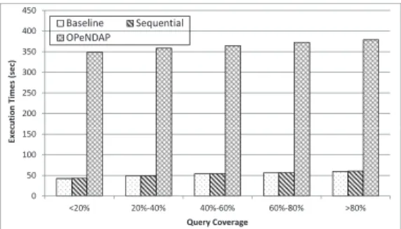
Figure 6 shows the execution time over different queries. The first bar in each group is the baseline of our current experiment, which contains two sub-parts, execution time of the intrinsic HDF5 query function, and the content-based filtering time. Since HDF5 library does not support subsetting based on data values, content-based filtering requires a full scan over the hyperslabs selected by the hyperslab selector. This baseline execution time is proportional to the amount of data subset. The second bar represents the execution time of our system. For type 2 and type 3 queries, we can see that it takes almost the same amount of

ϮϬϬ ϮϱϬ ϯϬϬ ϯϱϬ ϰϬϬ ϰϱϬ ĐƵƚ ŝŽ Ŷ dŝ ŵĞƐ ;ƐĞĐͿ ĂƐĞůŝŶĞ ^ĞƋƵĞŶƚŝĂů KWĞEW Ϭ ϱϬ ϭϬϬ ϭϱϬ фϮϬй ϮϬйͲϰϬй ϰϬйͲϲϬй ϲϬйͲϴϬй хϴϬй dž ĞĐ YƵĞƌLJŽǀĞƌĂŐĞ

Fig. 6. Performance Comparison for Type 2 and Type 3 Queries

time to perform hyperslab selection compared with the baseline, because the overhead of the additional dimension scale mapping is still quite trivial. The third bar shows the execution time of OPeNDAP. Without hyperslab selection support for subsetting, OPeNDAP has to scan the entire dataset to perform content-based filtering. Thus, both the data query cost and the data filtering cost are much higher than our system.

B. Parallelization of Subsetting Queries

As we have stated earlier, besides better performance and expressibility of our system over OPeNDAP, one of our advan-tages is the support for parallelization. In this subsection, we evaluate the performance improvements through parallelization of data subsetting operations. Our experiments were conducted on a cluster of multi-core machines. The system uses AMD Opteron(TM) Processor 8218 with 4 dual-core CPUs (8 cores in all). The clock frequency of each core is 2.6 GHz, and the system has a 12 GB memory. We have used up to 128 cores (16 nodes) for our study.

ϭϱϬ ϮϬϬ ϮϱϬ ϯϬϬ ĐƵƚŝ ŽŶ dŝŵ ĞƐ ;Ɛ ĞĐͿ ϭŶŽĚĞ ϮŶŽĚĞƐ ϰŶŽĚĞƐ ϴŶŽĚĞƐ ϭϲŶŽĚĞƐ Ϭ ϱϬ ϭϬϬ ϰ' ϴ' ϭϲ' ϯϮ' dž ĞĐ ĂƚĂƐĞƚ^ŝnjĞƐ

Fig. 7. Parallel Query Processing Times with Different Dataset Sizes

The first experiment evaluates the performance of parallel subsetting with different dataset sizes. In this experiment, the input queries simply fully scan the datasets. The experimental data sizes vary from 4 GB to 32 GB, while the number of nodes used for parallel subsetting varies from 1 to 16. Figure 7 shows the results as we scale the number of nodes. We can see that our system is capable of scaling the performance of processing such queries.

In the second experiment, we evaluated the performance of parallel subsetting. With different 3 types of query conditions, we generated 300 queries which cover different proportions of the dataset based on different dimensions. Figure 8 presents the results, which are divided into 5 coverage proportion groups. The experimental data sizes were 16 GB, and the number of nodes used for parallel subsetting varied from 1 to 16. We can see that with our optimized partitioning approach, which leads to a better data contiguity of partitions, the parallelization time for different

ϭϬϬ ϭϱϬ ϮϬϬ ϮϱϬ ĐƵƚŝŽŶ dŝŵĞ Ɛ; ƐĞ ĐͿ ϭŶŽĚĞ ϮŶŽĚĞƐ ϰŶŽĚĞƐ ϴŶŽĚĞƐ ϭϲŶŽĚĞƐ Ϭ ϱϬ ϭϬϬ фϮϬй ϮϬйͲϰϬй ϰϬйͲϲϬй ϲϬйͲϴϬй хϴϬй dž ĞĐ YƵĞƌLJŽǀĞƌĂŐĞ

Fig. 8. Parallel Query Processing Times with Different Queries

queries is approximately proportional to the amount of subsetting data.

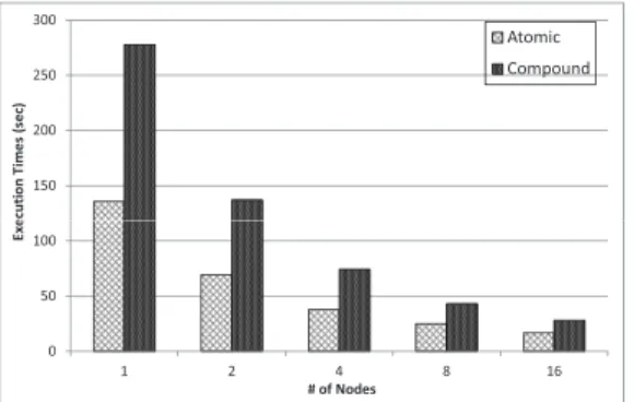
Since the pervious experiments didn’t involve any type 3 query on compound dataset, we conducted the third experiment to compare the performance of content-filtering over atomic datasets against compound datasets. In order to highlight the performance gap between the type 3 queries on atomic datasets and on compound dataset, we generated 100 queries which perform a pure content-filtering over the compound datasetcell. Figure 9 presented the results as we scaled the number of nodes from 1 to 16 for 16 GB datasets. We can see that the overhead of content-filtering over compound datasets is approximately as twice high as the one over atomic dataset. This is because that, although content-filtering is performed based on the value of a single data member within a compound data element, the entire compound data element has to be loaded first. By contrast, the content-filtering over atomic datasets can avoid the cost of loading the query-unrelated data (i.e. other data member(s) within a compound data element), since different atomic data is stored in separate datasets. The reason why the overhead ratio is close to 2 is that, in our scenario, the size of the experimental compound datatype is accidentally as twice large as either experimental atomic datatype. We believe that if the compound datatype consists of more data members, or the data member sizes become larger, the performance gap might become huger accordingly.

ϭϱϬ ϮϬϬ ϮϱϬ ϯϬϬ ĞĐ Ƶƚ ŝŽ Ŷdŝ ŵ ĞƐ; ƐĞ ĐͿ ƚŽŵŝĐ ŽŵƉŽƵŶĚ Ϭ ϱϬ ϭϬϬ ϭ Ϯ ϰ ϴ ϭϲ dž Ğ ηŽĨEŽĚĞƐ

Fig. 9. Performance Comparison of Content-Filtering over Atomic Datasets and Compound Datasets

C. Sequential and Parallel Performance of Aggregation Queries This subsection is designed to compare both the data transfer cost and the data aggregation performance between OPeNDAP and our system, by performing different types of data aggregation. Recall that OPeNDAP does not support data aggregation. Thus, to perform data aggregations with OPeNDAP, users have to first download all the data from the server side and then develop its

TABLE II

AGGREGATIONQUERYEXAMPLES Type Query Example

AG1 SELECT AVG(temperature), AVG(salinity) FROM MODB; AG2 SELECT COUNT(temperature) FROM MODB GROUP BY time

HAVING time>=319288;

AG3 SELECT MAX(temperature), MIN(temperature), MAX(salinity),_{MIN(salinity) FROM MODB GROUP BY layer;}

TABLE III

DATATRANSFERVOLUMECOMPARISON AGAINSTOPENDAP Aggregation Type Avg. Data Transfer Volume (byte)

OPeNDAP Our System

AG1 15,979,863,952 64

AG2 15,979,863,952 188

AG3 15,979,863,952 2040

own code to perform the aggregation at the client side. In contrast, our system supports parallel server-side data aggregation which can lead to a much smaller cost for both data transfer and data aggregation.

Table II shows aggregation types and examples used in our evaluation. We generated 100 aggregation queries and categorized them into three types: 1) AG1: query only includes aggregations; 2) AG2: query includes both aggregations and groupby with havingsubsetting; and 3) AG3: query includes both aggregations andgroupbywithouthavingsubsetting. To highlight the efficiency improvement of parallel data aggregation, we didn’t involve any WHEREclause in the queries in this experiment. The sizes of the experimental datasets were 16 GB.

One advantage of our parallel server-side data aggregation is the significant reduction in data transfer volume. This advantage is very likely to bring about considerable performance improve-ments when the server and the client need to communicate over the wide area network. Table III compares the total data volume that is transferred over the network between OPeNDAP and our system. We can see that, regardless of aggregation type, the entire dataset has to be transferred over the network before OPeNDAP performs data aggregation. On the other hand, in our system, AG1 has the smallest data transfer cost. This is because as noGROUP BYclause is involved, only a grand aggregation result is required to be transferred. Moreover, AG2 has smaller data transfer volume than AG3, because AG2 involvesHAVINGclause that will reduce the number of aggregation groups, and hence a smaller number of aggregation results are transferred. To conclude, for all the three aggregation types, our system demonstrated a tremendously smaller data transfer cost than OPeNDAP.

ϲϬ ϴϬ ϭϬϬ ϭϮϬ ϭϰϬ ĐƵƚŝ ŽŶ dŝŵ ĞƐ ;Ɛ ĞĐͿ KWĞEW ϮŶŽĚĞƐ ϰŶŽĚĞƐ ϴŶŽĚĞƐ ϭϲŶŽĚĞƐ Ϭ ϮϬ ϰϬ '/ '// '/// dž ĞĐ ŐŐƌĞŐĂƚŝŽŶdLJƉĞƐ

Fig. 10. Comparison of Data Aggregation Times

Besides the performance improvement in data transfer, our method can lead to a much smaller data aggregation cost. Our last experiment compared the data aggregation performance of

OPeN-DAP with our parallel system. We used up to 16 nodes to perform different types of aggregation queries over 16 GB datasets. The results presented in Figure 10 demonstrated a good speedup of our parallel aggregation approach against the OPeNDAP’s sequential aggregation, and a good scalability as the number of nodes increases. The relative speedups are demonstrated up to 8.13, 7.35 and 6.55, for the three types of aggregation queries, respectively.

VII. RELATEDWORK

The topics of scientific data management have attracted a lot of attention in recent years. Because of the large volume of work in this area, we concentrate on work specific to the tools or approaches that can be used with scientific data formats like HDF5, and then we provide a brief overview of the most significant other work.

OPeNDAP [8] supports data virtualization via a data access protocol and data representation. We have conducted extensive comparison of functionality and performance between our system and OPeNDAP. Barrodale Computing Services (BCS) [6] has developed a plug-in called the Universal File Interface (UFI) [5], which establishes a virtual table interface to allow Informix DBMS to transparently access HDF5 files as they were relational tables. However, it can support neither data aggregation nor par-allel query processing. The NetCDF Operator (NCO) library [3] and its parallel implementation [18] have been extended to support parallel query processing over NetCDF files. The queries supported by this tool have to be expressed in very specialized scripting languages, which unfortunately severely undermines their ease-of-use. MLOC [9] can optimize the storage layout of scientific data and hence facilitate queries based on coordinates, data values and even precision. However, it requires aforehand data transformation which may be prohibitively expensive, while our approach can directly manipulate on the original dataset. SciHadoop [7] and SciMATE [19] have integrated map-reduce and its variant with scientific library to enable map-reduce tasks over scientific data. While map-reduce can be used to implement selection and aggregation queries, SQL queries are simpler to write.

On the other hand, besides subsetting and aggregation, more well-known database techniques have been applied to scientific data management. Scientific Data Manager (SDM) employs the Meta-data Management System (MDMS) [14] and provides a high-level, user-friendly interface which interacts with database, to hide low-level parallel I/O operations for complex scientific processing. In comparison, our approach is more light-weight, and it can serve more HDF5 features such as dimension scale, compound datatype, and user metadata. FastQuery [11] utilizes parallel bitmap indexing to accelerate searches on scientific data files. By contrast, we focus on supporting various types of queries over scientific dataset with a standard high-level interface. In the future, we will extend our work by incorporating more database techniques such as indexing.

Scientific data management has drawn much attention lately. Several groups have articulated the requirements in this area [10], [13]. Recently, there has been a significant interest in extending (relational) database technology to support the need of (extreme-scale) scientific data [17], leading to multiple Extreme Scale Databases Workshops (XLDB). The requirements arising have been summarized in a position paper by Stonebraker [15], and now, an initial version of SciDB is available. While our approach focuses on providing database-like support to the users (i.e. user-defined subsetting and aggregations), the key difference in our approach is that the data is kept in its native form (e.g. flat-files, HDF5, or NetCDF), completely eliminating the need for loading the dataset into a database system. Our approach also provides a light-weight solution, which can be made available to different application domains more easily. The work presented in this paper can be viewed as an implementation of the more general data

virtualization approach introduced in our earlier work [20]. More recently, we reported a similar implementation for NetCDF [16]. The specific contributions of this work are in handling HDF5 features, like the more distributed metadata and the notion of hyberslabs. The design reported in this paper can optimize more complex queries also.

VIII. CONCLUSIONS

This paper describes implementation of a light-weight data management approach for scientific datasets stored in HDF5, which is one of the most popular scientific data formats. Our tool supports parallel data subsetting and aggregation in avirtual data viewthat is specified by SQL. Besides supporting selection over dimensions, which is also directly supported by HDF5 API, our system also supports queries based ondimension scales and/or data values. We have extensively evaluated our implementation and compared its performance and functionality against OPeN-DAP. We demonstrate that even for the queries that are directly supported in OPeNDAP, the sequential performance of our system is better. In addition, our system is capable of supporting a larger variety of queries, scaling performance by parallelizing the queries, and reducing wide area data transfers through server-side data aggregation.

REFERENCES [1] HDF5. http:// hdf.ncsa.uiuc.edu/HDF5/.

[2] HDF5 High-level APIs. http://www.hdfgroup.org/HDF5/doc/HL/. [3] NetCDF Operator (NCO). http://nco.sourceforge.net/.

[4] SQLite. http://wwww.sqlite.org.

[5] Universal File Interface (UFI). http://www.barrodale.com/bcs/universal-file-interface-ufi/.

[6] Barrodale Computing Services. http://www.barrodale.com/, 2010. [7] J. B. Buck, N. Watkins, J. LeFevre, K. Ioannidou, C. Maltzahn, N. Polyzotis,

and S. Brandt. SciHadoop: Array-based Query Processing in Hadoop. In

Proceedings of SC, 2011.

[8] P. Cornillon, J. Gallagher, and T. Sgouros. OPeNDAP: Accessing Data in a Distributed, Heterogeneous Environment.Data Science Journal, 2(0):164– 174, 2003.

[9] Z. Gong, T. Rogers, J. Jenkins, H. Kolla, S. Ethier, J. Chen, R. Ross, S. Klasky, and N. F. Samatova. MLOC: Multi-level Layout Optimization Framework for Compressed Scientific Data Exploration with Heterogeneous Access Patterns. InProceedings of ICPP, September 2012.

[10] J. Gray, D. T. Liu, M. Nieto-Santisteban, A. Szalay, D. J. DeWitt, and G. Heber. Scientific data management in the coming decade. SIGMOD Rec., 34:34–41, December 2005.

[11] C. Jerry, W. Kesheng, and Prabhat. FastQuery: A Parallel Indexing System for Scientific Data. InCLUSTER, pages 455–464. IEEE, 2011. [12] C. Johnson and R. Ross. Visualization and knowledge discovery: Report

from the DOE/ASCR workshop on visual analysis and data exploration at extreme scale. Technical report, Department of Energy Office of Science ASCR, Oct. 2007.

[13] R. Musick and T. Critchlow. Practical lessons in supporting large-scale computational science.SIGMOD Rec., 28:49–57, December 1999. [14] J. No, R. Thakur, and A. Choudhary. Integrating Parallel File I/O and

Database Support for High-Performance Scientific Data Management, 2000. [15] M. Stonebraker, J. Becla, D. Dewitt, K.-T. Lim, D. Maier, O. Ratzesberger, and S. Zdonik. Requirements for Science Data Bases and SciDB. In

Conference on Innovative Data Systems Research (CIDR), Jan. 2009. [16] Y. Su and G. Agrawal. Supporting User-Defined Subsetting and Aggregation

over Parallel NetCDF Datasets. InProceedings of CCGRID, pages 212–219, may 2012.

[17] A. S. Szalay, P. Z. Kunszt, A. Thakar, J. Gray, D. Slutz, and R. J. Brunner. Designing and mining multi-terabyte astronomy archives: the Sloan Digital Sky Survey. InProceedings of the 2000 ACM SIGMOD international conference on Management of data, pages 451–462, New York, NY, USA, 2000. ACM.

[18] D. Wang, C. Zender, and S. Jenks. Clustered Workflow Execution of Retargeted Data Analysis Scripts. InProceedings of CCGRID, pages 449– 458, Washington, DC, USA, may 2008. IEEE Computer Society. [19] Y. Wang, W. Jiang, and G. Agrawal. SciMATE: A Novel

MapReduce-Like Framework for Multiple Scientific Data Formats. InProceedings of CCGRID, pages 443–450, may 2012.

[20] L. Weng, G. Agrawal, U. Catalyurek, T. Kurc, S. Narayanan, and J. Saltz. An Approach for Automatic Data Virtualization. InProceedings of HPDC, pages 24–33, Washington, DC, USA, 2004. IEEE Computer Society.