A Skew-Normal Copula-Driven Generalized Linear Mixed Model for Longitudinal Data

(1)

Model for Longitudinal Data

Mohamad Elmasri

Department of Mathematics and Statistics

Concordia University

Montreal, QC

Presented in Partial Fulfillment of the Requirement for the Degree of

Master of Science in Mathematics

April 2012

c

(2)

This is to certify that the thesis prepared

By: Mohamad Elmasri

Entitled: A Skew-Normal Copula-Driven Generalized Linear Mixed

Model For Longitudinal Data

and submitted in partial fulfillment of the requirements for the degree of

Master of Science in Mathematics

complies with the regulations of the University and meets the accepted

standards with respect to originality and quality.

Signed by the final examining committee:

Examiner Dr. C. Hyndman Examiner Dr. Y. P. Chaubey Thesis Supervisor Dr. A. Sen Approved by

Chair of Department or Graduate Program Director

Dean of Faculty

(3)

A Skew-Normal Copula-Driven Generalized Linear Mixed

Model for Longitudinal Data

Mohamad Elmasri

Using the advancements ofArellano-Valle et al. [2005], which charac-terize the likelihood function of a linear mixed model (LMM) under a

skew-normal distribution for the random effects, this thesis attempt to

construct a copula-driven generalized linear mixed model (GLMM).

Assuming a multivariate distribution from the exponential family for

the response variable and a skew-normal copula, we drive a complete

characterization of the general likelihood function. For estimation, we

apply a Monte Carlo expectation maximization (MC-EM) algorithm.

Some special cases are discussed, in particular, the exponential and

gamma distributions. Simulations with multiple link functions are

shown alongside a real data example from the Framingham Heart

(4)

I would like to thank Professor Kalyan Das, Department of Statistics,

University of Calcutta for the proposition of the model, and my

super-visor, professor Arusharka Sen, for his patience explaining the model,

and his general guidance and knowledge that have aided me greatly

throughout my undergraduate and graduate studies. I am grateful to

Professor Yogendra Chaubey for his guidance and support during my

graduate studies and for reviewing this work. I am also grateful to

Professor Lea Popovic for all the discussions that guided me generally

and for the countless reference letters she wrote for me.

I am very grateful to all the friends I have, for the unconditional

sup-port, for all the good times we have spent together, for the cheers and

laughs we shared, and for baring with me during the hard times. Here

I must mention a few; Santiago, for the endless hours we spent in the

lab during my studies; Catherine and Maryam, for their warmth and

smiles, and for putting up with me during the hard times. Without

exception, I am fortunate to have your friendship.

Special thanks to my uncle Ghassan and his wife Racha, for their

(5)

(6)

Contents vi

List of Tables ix

List of Figures x

1 Introduction 1

1.1 The linear mixed model . . . 1

1.2 The skew-normal distribution . . . 4

1.2.1 Univariate skew-normal distribution . . . 5

1.2.2 Multivariate skew-normal distribution . . . 6

2 Modeling the joint distribution via a skew-normal copula 12 2.1 The model . . . 12

2.2 Skew-normal copula . . . 13

2.3 Autoregressive correlation matrix . . . 17

2.4 GLM framework for response variable and the maximum likelihood 20 2.4.1 Exponential family of distributions . . . 20

(7)

2.4.3 Response variable as a gamma distribution . . . 22

2.5 Graphical examples . . . 22

2.6 Likelihood function . . . 24

3 Numerical computation with EM-algorithm 27 3.1 Monte Carlo based EM algorithm . . . 27

3.2 Applying the MC E-step . . . 30

3.3 Applying the M-step . . . 34

3.4 Algorithm . . . 35

3.5 Special cases of EM algorithm . . . 36

3.5.1 Exponential marginal density with link η(x) =ex _{. . . . .} ₃₆

3.5.2 Exponential marginal density with link η(x) =x2 _{. . . . .} ₃₇

3.5.3 Exponential marginal density with link η(x) =x−1 _{. . . .} ₃₈

3.5.4 Gamma marginal density with link η(x) = ex . . . 40

3.5.5 Gamma marginal density with link η(x) = x2 . . . 41

3.5.6 Gamma marginal density with link η(x) = x−1 _{. . . .} ₄₂

4 Simulation and application 44 4.1 Simulation design . . . 44

4.1.1 Univariate model . . . 45

4.1.2 Bivariate model . . . 45

4.2 Simulation under special cases of link and distribution function . . 46

4.2.1 Exponential marginal density . . . 46

4.2.2 Gamma marginal density . . . 48

(8)

5 Conclusion and final remarks 54

Appendix A 55

.1 MCEM algorithm diagram . . . 55

(9)

4.1 Univariate model under and exponential distribution such that

E[Yi] = µi =eXiβ+bi and a variance-covariance matrix Σi(φ) with

φi = 0.15, ∀i . . . 47

4.2 Multivariate model under and exponential distribution such that

E[Yi] = µi =eXiβ+bi and a variance-covariance matrix Σi(φ) with

φi = 0.15, ∀i . . . 48 4.3 Multivariate model under a gamma distribution such thatE[Yi] =

µi =eXiβ+bi, where k is the shape parameter and is fixed to 3. A variance-covariance matrix Σi(φ) withφi = 0.15, ∀i . . . 49

4.4 Fitting of Framingham Heart Study cholesterol data with model

(4.3.2) using an exponential link and gamma distribution function,

the shape parameter k= 3. . . 52

4.5 Fitting of Framingham Heart Study cholesterol data comparison

(10)

2.1 Contour of a bivariate gamma distribution using the proposed

cop-ula method in (2.2) and (2.2.5) with shape parameter k = (2,3)T_, scale α= (1,1)T _{and different values of correlation coefficient}_ρ_{. .} ₂₃ 2.2 Contour of a bivariate gamma distribution using the proposed

cop-ula method in (2.2) and (2.2.5) with shape parameter k = (2,5)T, scale α= (1,1)T and different values of correlation coefficientρ. . 23

2.3 Contour of a bivariate gamma distribution using the proposed

cop-ula method in (2.2) and (2.2.5) with shape parameter k = (5,5)T_, scale α= (1,1)T _{and different value of correlation coefficient}_ρ_{. . .} ₂₄ 4.1 A univariate model with an exponential link and distribution

func-tion, where the log density ofY versus log(η(.)) are plotted on the x-axis; in bold and dotted lines respectively. (4.1a) compares a

sin-gle replication of the estimated model versus the real model, while

(11)

4.2 A multivariate model with an exponential link and distribution

function, where the log density of Y versus log(η(.)) are plotted on the x-axis; in bold and dotted lines respectively. (4.2a)

com-pares a single replication of the estimated model versus the real

model, while (4.2b) is a 100 Monte Carlo replications versus the

real model. . . 48

4.3 A multivariate model with an exponential link and gamma

distri-bution function, where the log density of Y versus log(η(.)) are plotted on the x-axis; in bold and dotted lines respectively. (4.3a)

compares a single replication of the estimated model versus the

real model, while (4.3b) is a 100 Monte Carlo replications versus

the real model. The shape parameter k = 3. . . 49

4.4 Fitting of Framingham Heart Study cholesterol data with model

(4.3.2) using an exponential link and gamma distribution function,

the shape parameter k = 3. The solid lines are the fitted model, while the histogram shows the frequency distribution of cholesterol

(12)

Introduction

1.1

The linear mixed model

The key component driving the development of linear mixed models is the ability

of such models to handle data with non-independent observations; a data

struc-ture where predictor/response variables are measured at more than one level.

Such structure is common with repeated observations, notably longitudinal data

in medical studies where patient characteristics are measured over varying times.

Because of the imposed dependence between observations from the same source,

the presumed independence of errors in linear models is in turn violated and the

Ordinary Least Square method fails to capture the characteristics of coefficients.

The first improvement on the linear model to accommodate hierarchical data

was proposed byFisher[1918], discussing the correlation between relatives through Mendelian inheritance. Fisher proposed the addition of the random effects term

to the linear model, which in turn relaxed the homoscedastic condition on error.

(13)

fixed effects and best linear prediction (BLUP).

To characterize the linear mixed model, define the different measurement

lev-els as units, and let Yi be an (ni×1) of observed response variable for sample unit i, i= 1, ...., m. Then Yi is defined as

Yi =Xiβ+Zibi+i, i= 1, . . . , m (1.1.1)

where Xi of dimension (ni×p) is the design matrix corresponding to the fixed effects β of dimension (p×1), Zi of dimension (ni×q) is the design matrix that incorporates the hierarchical variables as random effects, bi is the random effects

regression coefficients of dimension (q×1) and i of dimension (ni ×1) is the vector of random errors. Note that the terms in Zi represent a non-time variant

or categorical variables that constitute the hierarchical structure of the data.

Inferences from this model become slightly more tedious by the addition of

the random coefficient bi to the known error terms i. A general approach to

manage such complexity is by assuming independence between bi andi as follow

bi iid

∼ Nq(0, D), i

ind

∼ Nni(0, ψi) (1.1.2)

where D = D(α), ψi = ψi(γ), for all i = 1, . . . , m are associated dispersion

matrices depending on reduced parameters α and γ with possible variability

among -and within- individuals. Putting aside the independence assumption

between random effects and residual, the extra restrictiveness associated with

distribution function characteristics and structure of both bi and i is deemed to be unnecessary in many literature reviews. Although Butler and Louis [1992] have recently shown that the normality assumption has little effect on the fixed

(14)

effects estimates, this assumptions’ effect on the random effects estimates has

not been investigated until Verbeke and Lesaffre [1996]. They demonstrated

the use of a mixture of normals in estimating the random effects coefficients

by iterative means using the EM algorithm. Although their method has widely

expanded the boundaries of model estimation the drawbacks are more apparent

when observations depart from the normality assumption.

On the other hand,Zhang and Davidian [2001] adopted another approach us-ing the semi-parametric form in estimatus-ing random effects by extendus-ing Gallant and Nychka [1987] development of maximum likelihood semi-parametric

estima-tion procedures. Another iterative technique was demonstrated by Tao et al.

[1999], where they extended the work of Magder and Zeger[1996] by a predictive technique, they also compared non-parametric maximum likelihood (NPMLE)

and smoothed non-parametric maximum likelihood(SNPMLE) to Newton and

Zhang [1999] predictive recursion algorithm (PR). Finally, Arellano-Valle et al.

[2005], expanded the boundaries of the normally distributed random effects coeffi-cients and error to a skew-normal distribution, where the skew-normal

character-istics enhance the presumed distributions to include any slight departures caused

by skewness. Arellano-Valle et al. [2005]’s work was facilitated by the work of

Azzalini [1985], which constructed the distribution of a univariate skew-normal via an additive mixture of normal and half normal distributions. Arellano-Valle et al. [2005] expands on such concepts to deal with multivariate situations, where they have explicitly characterized the likelihood function and used a constrained

expectation maximization algorithm (CEM) to systematically produce coefficient

(15)

butions. In particular, given response variables Yij, i = 1, . . . n, j = 1, . . . , ni, we assume that Yi follows ni-variate distribution with a predefined mean and variance-covariance matrix. We will model such distribution by using ani-variate skew-normal copulaSNni(.) and integrating the random effects in the mean

struc-ture of the copula. Furthermore, we chose the variance-covariance matrix Σi to

be of an autoregressive structure in order to include the time-variant parameters.

Formally,

Yi|bi ∼M V(η(Xiβ+bi),Σi(φi, ti)) (1.1.3) where bi is the unit specific unobserved random effect, φi is the dispersion au-toregressive time-variant parameter and η(.) is a link function.

The thesis is organized as follow; Chapter 2 discusses the formation of the

univariate and multivariate skew-normal distribution. Chapter 3 introduces the

model and constructs the likelihood using a skew-normal copula within a GLM

framework. Chapter 4 discusses the use of numerical Monte Carlo EM-algorithm

to estimate parameters of the established model. Chapter 5 presents numerical

simulations and a real data example using the proposed model.

1.2

The skew-normal distribution

This thesis uses the following notations; φn(.|µ,Σ) and Φn(.|µ,Σ) to represent a n-variate normal probability density and distribution functions respectively, with location vector µ and scale (n×n) variance-covariance matrix Σ. Hence,

for µ = 0 and Σ = In the previous notations would simplify to an n-variate

standard normal probability density and distribution functions φn(.) and Φn(.) respectively. In addition, letSNn(.|µ,Σ, λ) andsnn(.|µ,Σ, λ) be an-variate

(16)

skew-normal distribution and density functions respectively, with skewness vector λ. Similarly, a n-variate standard skew-normal distribution and density functions

are represented by SNn(.|λ) and snn(.|λ) respectively. Finally, letHN(.) be the half normal distribution function.

The following two sections summarize previous work and advancements in

modeling a univariate and multivariate skew-normal distributions.

1.2.1

Univariate skew-normal distribution

Following Azzalini [1985], a random variable X has a skew-normal distribution with skewness parameter λ if density function is represented as

sn1(x|λ) = 2φ1(x)Φ1(λx) (−∞< x < ∞) (1.2.1) similarly by sn1(x|µ, σ2, λ) = 2φ1(x|µ, σ2)Φ1(λ x−µ σ ) (1.2.2) (−∞< x <∞), µ, σ ∈ <, µ <∞,0< σ <∞

Note that if λ = 0 then the density of X in (1.2.2) reduces to a normal

distribution. The proof that equation (1.2.1) is a true density function comes

from the following lemma

Lemma 1.2.1 Azzalini[1985] Letf be a symmetric density function with respect to 0, G an absolutely continuous distribution function such that G0 is symmetric with respect to 0, then

(17)

is a density function for any real λ.

Proof Let Y and X be independent random variables with density f and G0, respectively. Then

1/2 =P{X−λY <0}=EY(P{X < λy|Y =y}) =

Z ∞

−∞

G(λy)f(y) dy (1.2.4) Another characterization of the skew-normal is as follow

Proposition 1.2.1 Azzalini and Dalle-Valle[1996] IfY0 and Y1 are independent

N(0,1) variables and ξ∈(−1,1) Then

Z =ξ|Y0|+ p 1 +ξ2_Y 1 f ollows SN1(λ(ξ)) (1.2.5) where ξ= √λ 1+λ2.

1.2.2

Multivariate skew-normal distribution

Extensions to the univariate skew-normal distribution in equation (1.2.1) was

first proposed by Azzalini [1985] and expanded further by Azzalini and Dalle-Valle [1996]. Later on, many authors have worked on generalizing such findings to include a family of multivariate and skew-elliptical distributions. This

sec-tion states some relevant results in chronological order, and concludes with two

advancements and their proof.

Azzalini and Capitanio[1999] defined a multivariate skew-distribution by the following non-unique notation

(18)

wherefk(.) is the density corresponding to a l-dimensional elliptical distribution, defined in Definition (1.2.1), and Qis a skewing function such thatQ(z)≥0 and

Q(−z) = 1−Q(z), ∀z ∈ <k_{. Note that} _Q₍_._{) could equally be represented by}

Q(z) = ν(u(z)), for some function u : <k _{→ <} _{and some non-negative function}

ν :< → <, such thatu(−z) =−u(z), ∀z ∈ <k_{, and}_ν₍₋_u_{) = 1}₋_ν₍_u₎_, _∀_u_{∈ <}_. Also note, equation (1.2.6) is a generalization to (1.2.1).

Definition 1.2.1 Owen and Rabinovitch[1983] A random vectorX = (X1, . . . , Xp) is said to have a p-elliptical distribution if it has a density function fX(x) say, then fX(x) can be expressed in the form of

FX(x) = k|Ω|−1g

(x−µ)TΩ−1(x−µ)

for some function g(.)mapping from non-negative reals to non-negative reals, and

g(.)is independent ofk. Ωis a positive definite matrix , and µis the mean vector. Thus fX(x) is only a function of the quadratic form (x−µ)TΩ−1(x−µ), which is positive by definition.

Some advancements are represented in the work ofArellano-Valle et al.[2002], where they generalized the previous findings in (1.2.6) to a class of skew-symmetric

distributions starting with a family of special C-class symmetric distribution,

where C represents the class of all symmetric random vectors X with P(X =

(19)

inde-pendent, and sign(X)∼Um d

= uniform on {−1,1}m_{, such that}

Wi =      +1 if Xi >0 −1 if Xi ≤0 i= 1, . . . , m, , Um ∼ uniform on {−1,1}m. (1.2.7)

Hence to obtain a density of any arbitrary skew distribution, the following

notations hold

f(z|am) =Km−1fk(z)Qm(z), ∀z ∈ <k (1.2.8) where

Km =P(X >0) and Qm(z) = P(X >0|Z =z) (1.2.9)

for some random vectorsX andZ with dimensionsm×1 and k×1 respectively,

and with joint distribution, in which that Z has marginal density fk. Note that if X is a C-random vector thenKm =P(X >0) = 2−m which transforms (1.2.8) to

f(z|am) = 2mfk(z)Qm(z), ∀z ∈ <k (1.2.10) Finally, for convenience the following results are used in the later sections. A

modified version of Arellano-Valle and Genton[2005] states that

Definition 1.2.2 An n-dimensional random vectorX follows a skew-normal dis-tribution with location vectorµ∈ <n_{, dispersion matrix}_Σ_(a_n_×_n_{positive definite} matrix) and a skewness vector λ ∈ <n_{, if its pdf is given by}

snn(x|µ,Σ, λ) = 2φn(x|µ,Σ)Φ1(λTΣ−1/2(x−µ)), x∈ <n. (1.2.11) Remark 1.2.1 Note that since the condition that Φ1(−w) = 1−Φ1(w) for all

(20)

w ∈ < satisfies requirement (1.2.6) and hence is sufficient to guarantee that (1.2.11) is a pdf.

Azzalini and Dalle-Valle [1996] proposed a simplified parametrization to Φ1(.) in

(1.2.11) ofλ in terms of an arbitraryn×n positive definite matrix ∆. Let us say ∆ = Σ or ∆ =In , such thatδT∆−1δ <1 for some δ∈ <n then,

λ= ∆

1/2_δ

√

1−δT_∆−1_δ (1.2.12)

Arellano-Valle and Genton [2005] representation of the multivariate skew-normal distribution is basically a modification to (1.2.5) in Proposition (1.2.1),

combined with (1.2.12) yielding

Proposition 1.2.2 Arellano-Valle et al. [2005] Let W ∼SNn(λ) . Then

W =d δ|X0|+ (In−δδT)1/2X1, where δ =

λ

√

1 +λT_λ (1.2.13)

X0 ∼N1(0,1)independent of X1 ∼Nn(0,1)

Before proving the previous proposition the following lemma is needed.

Lemma 1.2.2 Arellano-Valle et al. [2005] Let Y ∼Np(µ,Σ) and X ∼Nq(ν,Ω) Then

φp(y|µ+Ax,Σ)φq(x|ν,Ω) =φp(y|µ+Aν,Σ +AΩAT)

×φq(x|ν+ ΛATΣ−1(y−µ−Aν),Λ)

(1.2.14)

(21)

Proof of Lemma (1.2.2) By letting z = y−µ−Aν and w = x−ν, we have after some standard algebraic operations

(z−Aw)TΣ−1(z−Aw) +wTΩ−1w=z(Σ +AΩAT)−1z

+ (w−ΛATΣ−1z)TΛ−1(w−ΛATΣ−1z),

Noting that |Σ +AΩAT_||_Λ_|₌_|_Σ_||_Ω_|_.

Proof of Proposition (1.2.2) Let W = δ|X0| + (In − δδT)1/2X1. Since

W||X0| ∼ Nn(δ|X0|, In−δδT) where |X0| ∼ HN(0,1) then by Lemma (1.2.2) it

follows that fW(w) = Z ∞ 0 2φn(w|δt, In−δδT)φ1(t)dt = Z ∞ 0 2φn(w|0, In)φ1(t|δTw,1−δTδ)dt = 2φn(w)Φ1( δT_w √ 1−δT_δ) Then W ∼SNn(λ) withλ= √ δ 1−δT_δ.

The following is another needed and useful proposition.

Proposition 1.2.3 Arellano-Valle et al. [2005] Suppose that Y|T =t∼Nn(µ+

dt,Ψ) and T ∼ HN1(0,1) (a standardized half-normal distribution). Let Σ =

Ψ +ddT. Then the joint distribution of (YT, T)T can be written as

fY,T(y, t|θ, λ) = 2φn(y|µ,Σ)φ1(t|ν, τ2)I{t >0} (1.2.15) where ν= d T_Ψ−1₍_y₋_µ₎ 1 +dT_Ψ−1_d and τ 2 ₌ 1 1 +dT_Ψ−1_d (1.2.16)

(22)

Proof The proof for Proposition (1.2.3) follows directly from knowing that the joint density of Y and T is

fY,T(y, t|θ, λ) = 2φn(y|µ+dt,Ψ)φ1(t)I{t >0}

and from algebraic manipulation by integrating t out we have

φn(y|µ+dt,Ψ) =φn(y|µ,Σ)Φ1(t|ν, τ2)

which concludes the proof. Consequently, the marginal distribution of Y of

(1.2.15) is given by

fY(y|θ, λ) = 2φn(y|µ,Σ)Φ1(

ν τ)

So far, the literature have presented multiple useful versions of constructing an

n-variate skew-normal distribution. Hence, to complete the set of findings and to draw some useful characteristic of this distribution, the following corollary gives

the expectation and variance ofSNn(.) and follows directly from previous results.

Corollary 1.2.1 Arellano-Valle et al. [2005] Let Y =d µ+ Σ1/2W, where, W ∼

SNn(λ). Then Y ∼SNN(µ,Σ, λ). Moreover, E[Y] =µ+ r 2 πΣ 1/2_{δ and V ar}_[_Y_{] = Σ}₋ 2 πΣ 1/2_δδT_Σ1/2_.

(23)

Modeling the joint distribution

via a skew-normal copula

2.1

The model

Instead of building an additive model similar to one presented in (1.1.1) one can

consider a general multivariate distribution(MV) of the form

Yi|bi ∼M V(η(Xiβ+bi),Σi(φi, ti)) (2.1.1) where Yi|bi is the response variable of the ith unit at time ti = (ti1, . . . , tini),

i = 1, . . . , m, j = 1, . . . , ni, the longitudinal data available for unit i is then

Yi = (Yi1, . . . , Yij, . . . , Yini)

T_. _Further, _x

i is a (ni × p) vector of explanatory variables for unit iat timeti,bi is the unobserved unit specific random effect and

β is a (p×1) vector of regression coefficients to be estimated.

(24)

via the same link function η(.). Therefore, let FYij(yij|xij, tij, bi, β) denote the

conditional marginal distribution function of the response variable Yij|bi, and

fYij(yij|xij, tij, bi, β) denote its density. We may assume for the sake of simplicity

that xij does not depend on ti or bi. Further, let Fb(bi|σb2) ∼ N1(0, σ2b) be the distribution of the unit specific random effect with density fb(.|σb2).

2.2

Skew-normal copula

After characterizing the joint and marginal conditional distributions ofYi|bi in the previous section, this section defines the general properties of a copula and more

specifically construct a skew-normal copula with the given marginal distributions

Yij|bi.

Definition 2.2.1 Nelsen [1999] C : [0,1]d → [0,1] is a d-dimensional copula if

C is a joint cumulative distribution function of a d-dimensional random vector on the unit cube [0,1]d _{with uniform marginals.}

For example, in a bivariate case C : [0,1]×[0,1] → [0,1] is a bivariate copula if C(0, u) = C(u,0) = 0, C(1, u) = C(u,1) = u and C(y1, y2) −C(x1, y2)−

C(y1, x2) +C(x1, x2)≥0 for all [x1, y1]×[x2, y2]⊆[0,1]×[0,1].

Definition 2.2.2 Dodge [2003] Suppose that a random variable X has a contin-uous distribution for which the cumulative distribution function is FX. Then the random variable W defined as

(25)

Considering definitions (2.2.1) and (2.2.2), a skew-normal copula specifies the

joint distribution ofYi|bi with specified marginal distributionsFYij(yij|.) as follow,

let

Zij ∼SN1(bi,1, λij) at time tij for unit i, then

Zi = (zi1, . . . , zij, . . . , zini)

T _∼_SN

ni(bi1,Σi, λi)

where Σi is a correlation matrix, which has all its diagonal elements equal to 1,

and 1 = (1, . . . ,1)T_{. For modeling the contribution of} _Y

i|bi, the results obtained in (1.2.11) allow us to utilize the standard formation of a copula in Definition

(2.2.1) and define a multivariate skew-normal copula as

Cbi i =C bi i (ui1, . . . , uni) =SNni(SN −1 1 (ui1), . . . , SN1−1(uini)|bi1,Σi, λi) (2.2.1) where uij ∼uniform(0,1).

From Definition (2.2.2) we have FYij(yij|.) ∼ uij similarly SN1(zij|.) ∼ uij,

therefore we can write

Yij =FY−ij1(uij|.) = F

−1

Yij(SN1(zij)|.)

Zij =SN1−1(uij) =SN1−1(FYij(yij|.))

(26)

The corresponding skew-normal copula density function conditioned on bi is

where zij =SN1−1(FYij(yij|.)|b1,1, λij), the density function becomes

fYi(yi1, . . . , yini|xi, β, bi,Σi,) = snni(z1i, . . . , zini|bi1,Σi, λi) ni Y j=1 fYij(yij|xij, β, bi) sn1(zij|bi,1, λij) (2.2.5)

The unconditional skew-normal copula density function is

fYi(yi1, . . . , yini|xi, β,Σi) = Z fYi(yi1, . . . , yini|xi, β, bi,Σi)fbi(0, σ 2 b)dbi (2.2.6) where fb(0, σb2)∼N1(0, σb2).

Note that the joint distribution of the response vectorYi|bihas not yet been ex-plicitly defined, all what is required so far is to exex-plicitly define that the marginal

(27)

cop-ula representing the joint distribution function of any multivariate distribution

by having all the marginals distribution functions specified. For this thesis we

define the marginals as as a member of the exponential family distributions, as

explained later in section (2.4). The next section proposes a modification to the

correlation matrix Σi to include the time dependence variable. Later we propose

a GLM framework for the response variable.

To conclude this section, the following summarize our model. Fori= 1, . . . , m

and j = 1, . . . , ni our model is of the form

Yi|bi ∼FYi(.|xi, β, bi, ti,Σi), Yij|bi ∼FYij(.|xij, β, bi, tij)

FYi(.|xi, β, bi, ti) =SNni(Zi|bi1,Σi, λi),where Zi = (Zi1, . . . , Zini)

T

Zij ∼SN1(bi,1, λij), Yij =Fij−1(SN1(zij|bi,1, λij)|xi, β, bi, ti,Σi), bi ∼N1(.|σb2) To facilitate comparison to other similar models, the model ofArellano-Valle et al. [2005] is stated as Yi =Xiβ+Zibi+i (2.2.7) bi iid ∼ SNq(0, D, λb), i iid ∼SNni(0, ψi, λei), i= 1, . . . , m

where bi is independent of i and,

Yi|bi ind

(28)

2.3

Autoregressive correlation matrix

To produce a more plausible model one needs to take into account the different

sources of random variation within observations. Such random variations could

be generally specified by the following.

(i) Random effects: by sampling at random from a population, multiple aspects of behavior could persist stochastically. Such is the case when the

average level of the response variable varies widely between different time

intervals. At some moments there could be a very low response, others could

have a higher response. Such behaviors could produce some bias within the

error.

(ii) Serial correlation: different observations from the same variable sam-pled at different time intervals could be highly correlated. For example, a

patient’s blood pressure measure repeatedly over time in a medical study.

Therefore, one needs to take into account a regressive correlation structure

of the error.

(iii) Measurement error: a general random error could be accounted for

be-tween observations. When two measurements are taken simultaneously from

a source, there could be a slight variation between them which causes a

ran-dom error.

Note that the random effect source of variation is already accounted for within

(29)

covariance matrix Σi presented in (2.1.1) could be modeled as a function of time

and a dispersion variable φi as

Σi = Σi(φi, ti) (2.3.1)

As a result, assuming an additive decomposition of the above sources in the

variance-covariance structure letting

Yij =Wi(yi1, . . . , yi(j−1), tij) +ij (2.3.2) whereWi(.) is a linear function composing the source of variation generated from the serial correlation to previous observations. Here, letij

iid

∼N(0, σ2_i) be sample

of ni independent copies of a stationary Gaussian process with mean zero and

variance σ2

i that represents the measurement error.

Since the response variables is of the formYi|bi = (Yi1, Yi2, . . . , Yini), define,Hi

as ni×ni matrix with (j, k)th element hijk=ρi(|tij −tik|),hijk is the correlation betweenYij andYikrepresented in the functionWi(.) above. Also, letIibeni×ni identity matrix. Since the marginal distribution of Yi|bi in (2.2.2) are assumed to have the same distribution family, the variance-covariance matrix ofYi|bi is easily constructed as

(30)

Now, σ_i2 is the variance of eachyij and the correlations amongst the Yi’s are determined by the autocorrelation function ρi(.) as

Cov(Yij, Yik) =σi2ρi(|tij −tik|) (2.3.4) The simplest form to express the serial correlation above is to assume an

explicit dependence of the currentYij on predecessorsYi(j−1), . . . , Yi1, which could

be modeled usingnthorder autoregressive model. For example, considering a first order autoregressive model as

yij =αiyi(j−1)+ij (2.3.5)

where ij as defined in (2.3.2)

Note that it would be difficult to give a closed interpretation of the α pa-rameter if the measurements are not equally spaced in time or when times of

measurements are not common to all units. One way of solving this issue to

implement an exponential autocorrelation function ρ(.), where

Cov(Yij, Yik) = σ2ie

−φi|tij−tik| _(2.3.6)

Furthermore, the correlation between two response variable becomes

Corr(Yij, Yik) =e−φi|tij−tik| (2.3.7) This correlation structure would later be used to construct a correlation

(31)

marginal response variables Yij|bi, henceforth, implemented in the copula struc-ture.

2.4

GLM framework for response variable and

the maximum likelihood

We have already defined implicitly the joint distribution of the response variable

Yi|bi. Moreover, we have modeled such joint distribution using a skew-normal copula by implementing a fist order autoregressive correlation structure using an

exponential autocorrelation function. For the sake of completeness and rigor, at

this stage we need to explicitly characterize the expression of the distribution

of Yi|bi defined in (2.1.1). To allow flexibility, this thesis establishes a general expression for the distribution being a member of the exponential family of

dis-tributions. Later on, both the exponential and gamma distributions are used in

modeling and simulation with different non-linear link functions.

2.4.1

Exponential family of distributions

Consider an over-dispersed exponential family of distributions, which is a

gener-alization of the exponential family and exponential dispersion model of

distribu-tions. It includes those probability distributions parameterized byθandτ, whose density functions can be expressed in the form

fY(y|θ, τ) = exp b(θ)T_T₍_y₎₋_A₍_θ₎ d(τ) +B(y, τ) (2.4.1)

(32)

where T(.), b(.), d(.), A(.) and B(.) are known functions and θ is the parameter relating to the mean of the model, τ is the dispersion parameter.

Furthermore, we consider a link function η(.) that relates to the mean of the model by

E(Y|bi) =η(Xβ+bi)

The above general distribution structure include many known distributions;

for example, Exponential, Gamma, Pareto, and Poisson distribution.

2.4.2

Response variable as an exponential distribution

By assuming the marginals of the response vector Yi|bi follow an exponential distribution as

fYij(yij|λ) = exp{−λyij + log(λ)}, yij ≥0

A(.) = log(λ) B(.) = 0 E(Yij) =µ= 1 λ =η(xijβ+bi) yij ≥0⇒µ=η(xijβ+bi)≥0 (2.4.2) then fYij(yij|xij, bi, β) = exp{ −yij η(xijβ+bi) −log(η(xijβ+bi))}, yij ≥0 (2.4.3) where log is the natural logarithm.

(33)

2.4.3

Response variable as a gamma distribution

Similarly, by assuming the marginals of the response vector Yi|bi follow gamma distribution as fYij(yij|α, k) = exp{− yij α −A(α, k) +B(yij, k)} yij ≥0 B(yij) = (k−1) log(yij) A(α, k) = klog(α) + log(Γ(k)) Γ(k) = (k−1)! k ≥0 E(Yij) = µ=kα=η(xijβ+bi) yij ≥0, k≥0⇒µ=η(xijβ+bi)≥0 (2.4.4) then fYij(yij|xij, bi, β) = exp − kyij η(xijβ+bi) −klog η(xijβ+bi) k −log(Γ(k)) + (k−1) log(yij) (2.4.5)

2.5

Graphical examples

This section presents a variety of bivariate contour plots to compare the

ap-proximation of the method proposed in section (2.2). Mainly, a gamma density

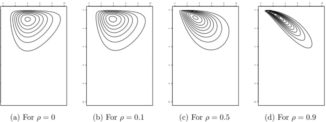
function is used under multiple configuration of shape parameter k and correla-tion ρ. In figures (2.1), (2.2) and (2.3) when ρ= 0, the contour plot is generated using two independent gamma densities; when theρ6= 0 the contour is generated using the copula method in (2.2) and (2.2.5).

(34)

0 2 4 6 8 10 0 2 4 6 8 10 (a) Forρ= 0 0 2 4 6 8 10 0 2 4 6 8 10 (b) Forρ= 0.1 0 2 4 6 8 10 0 2 4 6 8 10 (c) Forρ= 0.5 0 2 4 6 8 10 0 2 4 6 8 10 (d) Forρ= 0.9

Figure 2.1: Contour of a bivariate gamma distribution using the proposed copula method in (2.2) and (2.2.5) with shape parameterk = (2,3)T_{, scale} _α _{= (1}_,₁₎T and different values of correlation coefficient ρ.

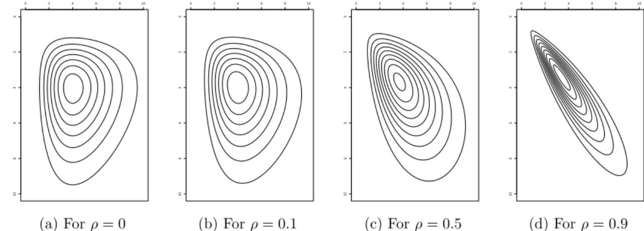
Figure 2.2: Contour of a bivariate gamma distribution using the proposed copula method in (2.2) and (2.2.5) with shape parameterk = (2,5)T, scale α = (1,1)T and different values of correlation coefficient ρ.

(35)

Figure 2.3: Contour of a bivariate gamma distribution using the proposed copula method in (2.2) and (2.2.5) with shape parameterk = (5,5)T_{, scale} _α _{= (1}_,₁₎T and different value of correlation coefficient ρ.

The similarities between figures produced using the two methods are very

apparent. Moreover, the application of copulas allows more flexibility, where any

correlation structure could easily be modeled even when the joint distribution is

not explicitly defined.

2.6

Likelihood function

The setting of longitudinal data over several units with repeated observations has

an additive characteristic of the log-likelihood across units. In particular, givenm

(36)

likelihood function as L(β,Σ) = m Y i=1 Z fYi(yi1, . . . , yini|xi, β,Σi, λi, bi)fbi(0, σ 2 b)dbi = Z m Y i=1 fYi(yi1, . . . , yini|xi, β,Σi, λi, bi) fbi(0, σ 2 b)dbi = Z m Y i=1 snni(z1i, . . . , zini|bi1,Σi, λi) ni Y j=1 fYij(yij|xij, β, bi) sn1(zij|bi,1, λij) fbi(0, σ 2 b)dbi = Z m Y i=1 Li(β, λi, σb,Σi|bi)fbi(0, σ 2 b)dbi (2.6.1)

where Li(β, λi, σb,Σi|bi) is the conditional likelihood. The exchangeability of the product and the integral comes as a result of the independent assumption between

units, similar to the independent assumption of errors in cross-sectional data.

The complete conditional log-likelihood transforms to

(37)

where from (2.2.5) we have

`i(β, λi,Σi, σbi|bi) = log(fYi(yi1, . . . yini|xi, β,Σi, λi, bi))

+ log(fbi(0, σb)) = log(snni(zi1, . . . , zini|bi1,Σi, λi)) + ni X j=1 log(fYij(yij|bi, β, xij)) − ni X j=1 log(sn1(zij|bi,1, λij)) + log(fbi(0, σb)) (2.6.3)

Note that we have delayed characterizing completely the log-likelihood

func-tion above to Chapter (3), where we introduce the MC-EM algorithm. Chapter

(3) also specifies the exact form of skew-normal density functions implemented

(38)

Numerical computation with

EM-algorithm

3.1

Monte Carlo based EM algorithm

The expectation-maximization algorithm is an iterative method for maximizing

the likelihood function. It consists of two steps from which the naming is derived;

an expectation (E-step) and a maximization step (M-step). The E-step computes

the expectation of the log-likelihood function over the given set of parameters

θ ∈ Θ and an unobserved parameter u with assumed density function g(u|x, θ). The M-step computes a new set of parameters that maximize the expected value

of the log-likelihood function found earlier in the E-step. Those two procedures

alternate on the path to find a set of parameters that maximize the likelihood

function. Furthermore, let θ donate the model parameters when complete-data

is available; hence,`(θ), θ∈Θ donates the complete-data log-likelihood function and Q(θ|θ0) the expected complete-data log-likelihood. Therefore both steps are

(39)

as follow

• E-step: Computes Q(θ|θ(r)) =E_u|θ(r)[`(θ)|θ(r)] as a function of θ. • M-step: Find θ(r+1) _{such that} _Q₍_θ(r+1)_|_θ(r)_{) =}_max

θ∈ΘQ(θ|θ(r)).

Theoretically, the log-likelihood function `(.) under the found parameter set θ(r)

should converge to a local or global maximum.

The EM-algorithm has been used widely in literature under different naming

conventions. Nevertheless, one of the earliest explanations of such method was

published by Dempster et al. [1977], where they generalized earlier attempts and sketched a convergence analysis for a wider class of problems. Since then,

numerous uses of such method have been unified under the name of EM-algorithm.

An advancement ofMeng and Rubin[1993] studies computational difficulties encountered while computing the M-step, where they proposed smaller

maximiza-tion steps over the parameter space. They argued that instead of maximizing the

whole set of parameters one can maximize in a sequential manner a subset of

parameters independently, while the other subset is held fixed. Such

modifica-tion is called a constrained maximizamodifica-tion step (CM). Theoretically, as long as

the maximization is applied on the whole set of parameters the algorithm should

reach convergence. This modification is referred to as an ECM-algorithm.

A second important advancement to the EM-algorithm was proposed by Wei

(40)

where u is the unobserved variable and R is relatively a large sample size. It is important to mention the work of Wu [1983] which studied the conver-gence properties of the EM algorithm. Wu [1983]’s work elaborates on Dempster et al. [1977] by clearly indicating a set of conditions that govern the convergence of EM-algorithm to a stationary point, whether a global or a local maximum.

Some of those conditions are; insuring that Q(θ|θ0) defined (3.1.1) is continuous on both θ and θ0; the set of parameters to be estimated θ0 belong to a compact space, let’s say Ω0; and the log-likelihood is bounded. The bound condition of

the proposed log-likelihood depends severely on the initial starting point of the

EM-algorithm, where it involves terms like log(|Σi|) → −∞ for very small |Σi|, shown later in equation (3.2.13), where |.| is the determinant. Heuristic method of initiating the algorithm from different starting points was successfully used by

Arellano-Valle et al.[2005], and considering the similarity of our model to theirs, a similar approach has been used here. Nevertheless, more analytical research

has to be undergone in order to prove theoretically the compactness of Ω0 and

the continuity of Q(θ|θ0), especially for the dispersion parameter φi in (2.3.1), since it is shown to be convoluted in the term |Σi|. This thesis would mainly focus on implementing the EM-algorithm heuristically with hope to show more

(41)

the proposed model above.

3.2

Applying the MC E-step

Let θ(r) _{= (}_β(r)_,_Σ(r)

i , σ

(r)

b , λ

(r)

i ) be the parameters of the rth EM iteration, then the E-step for unit i at (r+ 1) EM iteration is

whereb(_ij)is thejth_{sample generated from the distribution of}_b

i|zi, θ(r),Ridonates the number of replication on the ith _{unit. Hence,}

Q(θ|θ(r)) = m

X

i=1

Qi(θ|θ(r)) (3.2.2)

So far we haven’t explicitly defined the distribution of bi|Zi. Nevertheless, we have mapped the response variablesYi|bi to a skew-normal copula in Section (2.2) using a standard skew-normal marginal distributions as in equation (2.2.1) via

the link in (2.2.2). Similarly, we can use a conditional skew-normal distributional

asZij|bi ∼SN1(bi,1, λij), which byAzzalini[1985] and definition (1.2.2), for each

j, has its pdf in the following form

(42)

Alternatively, by Proposition (1.2.3), we can write for any given vi Zij|vi, bi ∼N1(bi+δijvi,1−δij2) (3.2.4) vi ∼HN1(0,1) bi ∼N1(0, σb2) where δij = λij q 1 +λ2 ij

Similarly, in a multivariate case, take Zi|bi ∼ SNni(biI,Σi, λi), where Σi has

all its diagonal elements as 1, we have

fZi|bi(zi, bi|,Σi, λi) = 2φni(zi|bi1,Σi)Φ1(λ

T_Σ−1/2

i (zi−bi1)) (3.2.5)

and arguing as earlier, we write

Zi|vi, bi ∼Nni(bi1 + Σ 1/2 i δ ∗ ivi,Σ 1/2 i (I−δ ∗ iδ ∗ i T )Σ1_i/2) (3.2.6) vi ∼HN1(0,1), bi ∼N1(0, σb2) where Σ1_i/2δ_i∗ = _p λi 1 +λT i λi

Proposition 3.2.1 given the settings in (3.2.6)then the conditional density func-tion of bi|zi, vi is specified by

(43)

where τ_i2 = ( 1 σ2 b + 1TΨ−_i 11)−1, Ψi = Σ 1/2 i (I−δ ∗ iδ ∗t i )Σ 1/2 i

Proof Algebraic manipulation with conditional densities yields

now by the assumption of independence between bi and vi, and noting that

fzi|vi = Z fzi|bi,vifbidbi = Z Nzi ni(bi1 + Σ 1/2 i δ ∗ ivi,Ψi)N1bi(0, σ 2 b)dbi By Lemma (1.2.2) = Z Nzi ni(Σ 1/2 i δ ∗ ivi,Ψi+ 1σb21 T )Nbi 1 (τ 2 i1 T Ψ−_i 1(zi−Σ1i/2δ ∗ ivi), τ 2 i)dbi =Nzi ni(Σ 1/2 i δ ∗ ivi,Ψi+ 1σb21 T₎ (3.2.9)

we have by (3.2.8) and (3.2.9) and Lemma (1.2.2)

fbi|zi,vi = Nzi ni(bi1 + Σ 1/2 i δ ∗ ivi,Ψi)N1bi(0, σb2) fzi|vi = N zi ni(Σ 1/2 i δi∗vi,Ψi+ 1σ2b1T)N bi 1 (τi21TΨ −1 i (zi−Σi1/2δi∗vi), τi2) fzi|vi = fzi|vi×N bi 1 (τi21TΨ −1 i (zi−Σ 1/2 i δ ∗ ivi), τi2) fzi|vi =Nbi 1 (τ 2 i 1 T_Ψ−1 i (zi−Σ 1/2 i δ ∗ ivi), τi2) (3.2.10)

Moreover, by applying algebraic manipulation to equation (3.2.7), and using

the proof results of Proposition (1.2.3), we have

bi|zi ∼SN1 τ_i21TΨ−_i 1zi, τi2 1 +τ_i2(1TΨ−_i 1Σ1_i/2δ∗_i)2 , λbi (3.2.11)

(44)

where τ2

i and Ψi as defined in (3.2.7) ,and λbi =−τi1

T_Ψ−1 i Σ 1/2 i δ ∗ i.

For clarity, after the modification proposed in (3.2.3) and (3.2.5), the

log-likelihood function in (2.6.3) is now defined as

`i(β, λi,Σi, σbi|yi, xi, bi) = log(snni(zi1, . . . , zini|Σi, λi, bi)) + ni X j=1 log(fYij(yij|bi, β, xij)) − ni X j=1 log(sn1(zij|bi, λij)) + log(fbi(0, σb)) (3.2.12)

By the characterization in (3.2.4) and (3.2.6) that are found through Proposition

(1.2.3), we can introduce a dummy variable vi ∼ HN(0,1) and rewrite the log-likelihood as `i(β, λi,Σi, σbi|yi, xi, bi) = log(Nni(zi1, . . . , zini|bi1 + Σ 1/2 i δ ∗ ivi,Ψi)) + ni X j=1 log(fYij(yij|bi, β, xij)) − ni X j=1 log(N1(zij|bi+δijvi,1−δij2)) + log(fbi(0, σb)) ∝ −1 2log|Σi| − 1 2(zi−bi1−Σ 1/2 i δ ∗ ivi)TΨ−i 1(zi−bi1−Σ 1/2 i δ ∗ ivi) + ni X j=1 log(fYij(yij|bi, β, xij)) − 1 2 ni X j=1 log(1−δ_ij2)−1 2 ni X j=1 (zij −bi−δijvi)2 (1−δ2 ij) − 1 2log(σb)− 1 2 b2 i σ2 b (3.2.13) whereδij = λij √ 1+λ2 ij

, and|Σi|represents the determinant. Ψi = Σ

1/2 i (I−δ ∗ iδ ∗t i )Σ 1/2 i and Σ1_i/2δ∗_i = √ λi 1+λT_iλi .

(45)

3.3

Applying the M-step

This step maximizes Q(θ|θ(r)) to produce an update estimate θ(r+1). Consider the score function

∂ ∂θQ(θ|θ (r)_{) =} ∂ ∂θ m X i=1 Qi(θ|θ(r)) = m X i=1 Ri X j=1 1 Ri ∂ ∂θ`i(θ|xi, yi, b (j) i ) (3.3.1)

Following the results obtained in equation (2.6.3), and by settingθ = (β, σb,Σi, λi) we have partial derivatives as:

∂ ∂σb Q(θ|θ(r)) = m X i=1 Ri X j=1 1 Ri − 1 2σb +b 2(j) i σ3_b (3.3.2)

maximizing over the domain by setting the above equation to zero yields

ˆ σ2 b = 2 m m X i=1 Ri X j=1 b2(_i j) Ri (3.3.3) Moreover, ∂2 ∂σ2 b Q(θ|θ(r)) = m X i=1 Ri X j=1 1 Ri 1 2σ2 b − 3b 2(j) i σ4 b (3.3.4) I(σb) = −E ∂2 ∂σ2 b Q(θ|θ(r)) = m5 2σ2 b (3.3.5)

where I(.) is the Fisher information coefficient, and,

∂2

∂σb∂β

(46)

∂2

∂β∂σb

Q(θ|θ(r)) = 0 (3.3.7)

Moreover, since the term involving the parameter φi in the log-likelihood is sep-arate from terms involving β and σb, we have

∂2 ∂φ∂βQ(θ|.) = ∂2 ∂φ∂σb Q(θ|.) = ∂ 2 ∂σb∂φ Q(θ|.) = ∂ 2 ∂β∂φQ(θ|.) = 0 (3.3.8)

Form (3.3.4), (3.3.6), (3.3.7) and (3.3.8), the Hessian matrix is

The subsections of section (3.5) present a closed form of the parameterβ max-imization scheme. Moreover, since the partial derivatives of the other parameters

are not quite trivial, a grid search algorithm is applied to maximize the likelihood

over the parameter space.

3.4

Algorithm

The algorithm consists of the following steps

(i) Obtain an initial estimate of θ(0) _{from the complete likelihood case and set}

b(0)_i = 0.

(ii) At the (r+ 1)-th iteration, obtain MC sample onbi.

(47)

plete data optimization technique as

θ(r+1) = arg max θ(r) Q(θ|θ

(r)₎

(iv) Continue steps (ii) & (iii) until convergence.

For more details see algorithm (1) in appendix (.1).

3.5

Special cases of EM algorithm

This section presents a compete E-step and M-step for the distributions

consid-ered in section (3.2) and (3.3) under different link functionsη(.) by following the GLM framework that is proposed in section (2.4). In each section an explicit

marginal density function of Yi|bi is stated along with the log-likelihood charac-terized in (3.2.13) and some partial derivatives. fYij(yij|.) represents the marginal

density of uniti, observationj of the joint densityYi|bi,D(.) is a diagonal matrix and I(.) is the Fisher information coefficient.

3.5.1

Exponential marginal density with link

η(x) =

e

x

fYij(yij|xij, bi, β) = exp{

−yij

η(xijβ+bi)

(48)

`i(β, λi,Σi, σbi|yi, xi, bi)∝ − 1 2log|Σi| − 1 2(zi−bi1−Σ 1/2 i δ ∗ ivi)TΨ−i 1(zi−bi1−Σ 1/2 i δ ∗ ivi) − 1 2 ni X j=1 log(1−δ_ij2)−1 2 ni X j=1 (zij −bi−δijvi)2 (1−δ2 ij) + ni X j=1 {−yije−xijβ−bi−xijβ−bi} − 1 2log(σb)− 1 2 b2 i σ2 b (3.5.2) whereδij = √λij 1+λ2 ij

, and|Σi|represents the determinant. Ψi = Σ1_i/2(I−δ∗_iδ_i∗t)Σ1_i/2 and Σ1_i/2δ∗_i = √ λi

1+λT iλi

Therefore, the marginal partial derivatives defined in (3.3.1) become

∂ ∂βì(β, λi,Σi, σbi|yi, xi, bi) = ni X j=1 xij{yije−xijβ−bi−1} (3.5.3) ∂2 ∂β2ì(β, λi,Σi, σbi|yi, xi, bi) = ni X j=1 −x2_ijyije−xijβ−bi (3.5.4) I(β) = m X i=1 −E ∂2 ∂β2ì(β, λi,Σi, σbi|yi, xi, bi) = m X i=1 ni X j=1 x2_ij (3.5.5) ˆ β =−(XTX)−1XT(log(D−1(Y)1) +bI) (3.5.6) where 1 = (1,1, . . . ,1)T_.

3.5.2

Exponential marginal density with link

η(x) =

x

2

−yij

η(xijβ+bi)

(49)

`i(β, λi,Σi, σb|yi, xi, bi)∝ − 1 2log|Σi| − 1 2(zi−bi1−Σ 1/2 i δ ∗ ivi)TΨ−i 1(zi−bi1−Σ 1/2 i δ ∗ ivi) − 1 2 ni X j=1 log(1−δ_ij2)− 1 2 ni X j=1 (zij −bi−δijvi)2 (1−δ2 ij) + ni X j=1 {−yij(xijβ+bi)−2 −2 log (xijβ+bi)} − 1 2log(σb)− 1 2 b2 i σ2 b (3.5.8) whereδij = λij √ 1+λ2 ij

1/2 i (I−δ∗iδi∗t)Σ 1/2 i and Σ1_i/2δ∗_i = √ λi 1+λT iλi

Therefore, the marginal partial derivatives defined in (3.3.1) becomes

∂ ∂βì(β, λi,Σi, σb|yi, xi, bi) =− ni X j=1 2xij{ yij (xijβ+bi)3 − 1 xijβ+bi } (3.5.9) ∂2 ∂β2ì(β, λi,Σi, σb|yi, xi, bi) =− ni X j=1 2x2_ij{ 3yij (xijβ+bi)4 − 1 (xijβ+bi)2 } (3.5.10) I(β) = m X i=1 −E ∂2 ∂β2ì(β, λi,Σi, σb|yi, xi, bi) = m X i=1 ni X j=1 4x2 ij (xijβ+bi)2 (3.5.11)

3.5.3

Exponential marginal density with link

η(x) =

x

−1

−yij

η(xijβ+bi)

(50)

`i(β, λi,Σi, σbi|yi, xi, bi)∝ − 1 2log|Σi| − 1 2(zi−bi1−Σ 1/2 i δ ∗ ivi)TΨ−i 1(zi−bi1−Σ 1/2 i δ ∗ ivi) − 1 2 ni X j=1 log(1−δ_ij2)−1 2 ni X j=1 (zij −bi−δijvi)2 (1−δ2 ij) + ni X j=1 {−yij(xijβ+bi) + log (xijβ+bi)} − 1 2log(σb)− 1 2 b2 i σ2 b (3.5.13) whereδij = √λij 1+λ2 ij

, and|Σi|represents the determinant. Ψi = Σ1_i/2(I−δ∗_iδ_i∗t)Σ1_i/2 and Σ1_i/2δ∗_i = √ λi

1+λT iλi

∂ ∂βì(β, λi,Σi, σbi|yi, xi, bi) =− ni X j=1 xij{yij − 1 xijβ+bi } (3.5.14) ∂2 ∂β2ì(β, λi,Σi, σbi|yi, xi, bi) = − ni X j=1 x2_ij (xijβ+bi)2 (3.5.15) I(β) = m X i=1 −E ∂2 ∂β2ì(β, λi,Σi, σbi|yi, xi, bi) = m X i=1 ni X j=1 x2_ij (xijβ+bi)2 (3.5.16) ˆ β = (XTX)−1XT(D−1(Y)1−b1) (3.5.17) where 1 = (1,1, . . . ,1)T_.

(51)

3.5.4

Gamma marginal density with link

η(x) =

e

x

Similar to the above, using equation (2.4.4), we have

fYij(yij|xij, bi, β) = exp{ −ke

(−xijβ−bi)_y

ij −k(xijβ+bi) +klog(k)

−log(Γ(k)) + (k−1) log(yij)}

(3.5.18)

and the unit i specific marginal log-likelihood defined in (2.6.3) becomes,

`i(β, λi,Σi, σbi|yi, xi, bi)∝ − 1 2log|Σi| − 1 2(zi−bi1−Σ 1/2 i δ ∗ ivi)TΨ−i 1(zi−bi1−Σ 1/2 i δ ∗ ivi) − 1 2 ni X j=1 log(1−δ_ij2)−1 2 ni X j=1 (zij −bi−δijvi)2 (1−δ2 ij) + ni X j=1 {−ke(−xijβ−bi)_y ij −k(xijβ+bi) +klog(k) −log(Γ(k)) + (k−1) log(yij)} − 1 2log(σb)− 1 2 b2 i σ2 b (3.5.19) whereδij = λij √ 1+λ2 ij

1/2 i (I−δ ∗ iδ ∗t i )Σ 1/2 i and Σ1_i/2δ∗_i = √ λi 1+λT iλi

∂ ∂β`i(β, λi,Σi, σbi|yi, xi, bi) = ni X j=1 kxij{yije−xijβ−bi −1} (3.5.20) I(β) = m X i=1 −E ∂2 ∂β2`i(β, λi,Σi, σbi|yi, xi, bi) = m X i=1 ni X j=1 kx2_ij (3.5.21)

(52)

ˆ

β =−(XTX)−1XT(log(D−1(Y)1) +bI) (3.5.22) where 1 = (1,1, . . . ,1)T

3.5.5

Gamma marginal density with link

η(x) =

x

2

fYij(yij|xij, bi, β) = exp{ −k(xijβ+bi)

−2_y

ij + 2klog(xijβ+bi) +klog(k)−log(Γ(k)) + (k−1) log(yij)}

(3.5.23)

`i(β, λi,Σi, σbi|yi, xi, bi)∝ − 1 2log|Σi| − 1 2(zi−bi1−Σ 1/2 i δ ∗ ivi)TΨ−i 1(zi−bi1−Σ1i/2δ ∗ ivi) − 1 2 ni X j=1 log(1−δ_ij2)−1 2 ni X j=1 (zij −bi−δijvi)2 (1−δ2 ij) + ni X j=1 {−k(xijβ+bi)−2yij + 2klog(xijβ+bi) +klog(k) −log(Γ(k)) + (k−1) log(yij)} − 1 2log(σb)− 1 2 b2 i σ2 b (3.5.24) whereδij = λij √ 1+λ2 ij

∂ ∂β`i(β, λi,Σi, σb|yi, xi, bi) = ni X j=1 2kxij{ yij (xijβ+bi)3 + 1 xijβ+bi } (3.5.25) I(β) = m X −E ∂2 `(β, λ,Σ, σ |y, x, b ) = m X ni X 4kx2_ij (3.5.26)

(53)

3.5.6

Gamma marginal density with link

η(x) =

x

−1

Similar to the above, using equation (2.4.4), we have

fYij(yij|xij, bi, β) = exp{ −k(xijβ+bi)yij +klog(xijβ+bi)+

klog(k)−log(Γ(k)) + (k−1) log(yij)}

(3.5.27)

`i(β, λi,Σi, σbi|yi, xi, bi)∝ − 1 2log|Σi| − 1 2(zi−bi1−Σ 1/2 i δ ∗ ivi)TΨ−i 1(zi−bi1−Σ 1/2 i δ ∗ ivi) − 1 2 ni X j=1 log(1−δ_ij2)−1 2 ni X j=1 (zij −bi−δijvi)2 (1−δ2 ij) + ni X j=1 {−k(xijβ+bi)yij +klog(xijβ+bi)+

klog(k)−log(Γ(k)) + (k−1) log(yij)}

− 1 2log(σb)− 1 2 b2 i σ2 b (3.5.28) whereδij = λij √ 1+λ2 ij

∂ ∂β`i(β, λi,Σi, σbi|yi, xi, bi) = ni X j=1 kxij{−yij + 1 xijβ+bi } (3.5.29) I(β) = m X i=1 −E ∂2 ∂β2`i(β, λi,Σi, σbi|yi, xi, bi) = m X i=1 ni X j=1 kx2 ij (xijβ+bi)2 (3.5.30) and similarly ˆ β = (XTX)−1XT(D−1(Y)1−b1) (3.5.31)

(54)

(55)

Simulation and application

4.1

Simulation design

To assess the efficiency of the proposed likelihood and model above multiple

key statistics are needed. Two different model setting are chosen for inference

and assessment, a univariate model and a bivariate model. A unified simulation

structure is selected as the number of units to be fixed to 5, such thati= 1, . . . ,5, and under each simulation the number of observation is chosen randomly from

uniform distributionni ∼U(50,250). Once the number of units and observations per unit are decided, the per unit variance-covariance matrix is constructed as a

first order autoregressive model as in (2.3.6), with a choice ofφi = 0.15 ∀i. Note that in the case of φi = 0 the autoregressive structure reduces to an independent multivariate distribution. Finally, σb = 2.

(56)

4.1.1

Univariate model

Xi is generated from Nni(0, Ini×ni),φi = 0.15 ∀i,β = 3, and bi ∼N1(0, σb = 2).

Moreover, the time difference per observation within each unit is set to a unit

difference, i.e, in (2.3.6), e−φi|tij−tik| _{would reduce to}

e−φi|tij−tik|₌      e−φi _if _|_j₋_k_|_{= 1} 1 if j =k (4.1.1)

Therefore the response variable is generated from

Yi ∼M V(η(Xiβ+bi),Σi(φi)) (4.1.2)

with a chosen multivariate distribution and link function as in section (3.5).

4.1.2

Bivariate model

This model investigates the convergence under an extra binary variabletij, which in some cases could represent a measurement deviation under th existence of

certain events. Here tij = 1 for j ≤ 150 and tij = 0 for all j > 150. Similarly as above Xi is generated from Nni(0, Ini×ni), φi = 0.15 ∀i, β = (3,2)

T_{, and}

bi ∼ N1(0, σb = 2). Moreover, the time difference per observation within each unit is set to a unit difference. The response variable is then is generated from

Yi ∼M V(η([Xi, ti]β+bi),Σi(φi)) =M V(η(3Xi+ 2ti+bi),Σi(φi)) (4.1.3) The original correlation matrix Σi is used alongside original values ofλiandbi

(57)

to simulate a set of random variablesZi|bi defined in (3.2.5). Using those random variables and the inverse transformation method introduced in (2.2.2) along with

the desired marginal densities and link function to generate Yi|bi. Finally to initialize each simulation we set the initial vectors to β(0) _{= 0,} _λ(0)

i = 0, σb2(0) = 1

and φ(0)_i = 0.5. In each iteration, the Monte Carlo sampling from b(k)_|_Z _{is set to}

300 and gradually increases while algorithm (1) is run until convergence.

4.2

Simulation under special cases of link and

distribution function

Similar to section (3.5) and the special cases presented, this simulation presents

both models, a univariate and a bivariate, under an exponential link function

η(x) = ex_.

Note that all tables in this section represent a simulation of 100 Monte Carlo

data sets, where MC Mean and MC SD represent the Monte Carlo mean and

standard deviation. MSE represents the average standard error between Monte

Carlo simulation and the true value of the parameter. EC represents the

empir-ical coverage probability computed using Fisher information matrix assuming a

95% confidence interval. True values are shown in parentheses (.) next to the parameter symbol, i.e, β(3) implies original β parameter is set to 3.

4.2.1

Exponential marginal density

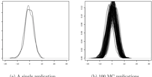
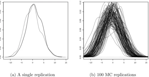
Before jumping to a complete simulation analysis, figure (4.1) below depict the

(58)

sim-ulated data set, using a univariate model with an exponential link and distribution

function. In addition, (4.2) depicts similar analysis under a multivariate model.

−20 −10 0 10 20 30 0.00 0.02 0.04 0.06 0.08 0.10 0.12

(a) A single replication

−20 −10 0 10 20 30 0.00 0.02 0.04 0.06 0.08 0.10 0.12 (b) 100 MC replications

Figure 4.1: A univariate model with an exponential link and distribution function, where the log density of Y versus log(η(.)) are plotted on the x-axis; in bold and dotted lines respectively. (4.1a) compares a single replication of the estimated model versus the real model, while (4.1b) is a 100 Monte Carlo replications versus the real model.

Moreover, table (4.1) and (4.2) represent the parameter estimation under the

univariate and multivariate model respectively.

Table 4.1: Univariate model under and exponential distribution such thatE[Yi] =

µi =eXiβ+bi and a variance-covariance matrix Σi(φ) withφi = 0.15, ∀i

Parameters MC Mean MC SD MSE EC

β(3) 2.91 0.02 0.01 0.54

E[b](0) 0.08 0.18 -

-σb(2) 2.15 0.41 0.19 0.99

(59)

−20 −10 0 10 20 30 0.00 0.02 0.04 0.06 0.08 0.10 0.12

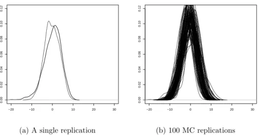
Figure 4.2: A multivariate model with an exponential link and distribution func-tion, where the log density of Y versus log(η(.)) are plotted on the x-axis; in bold and dotted lines respectively. (4.2a) compares a single replication of the estimated model versus the real model, while (4.2b) is a 100 Monte Carlo replications versus the real model.

Table 4.2: Multivariate model under and exponential distribution such that

E[Yi] = µi = eXiβ+bi and a variance-covariance matrix Σi(φ) with φi = 0.15,

∀i

β1(3) 3.03 0.16 0.002 0.99

β2(2) 1.53 0.64 0.63 0.20

E[b](0) -0.04 0.09 -

-σb(2) 1.99 0.43 0.18 0.93

φ(0.15) 0.38 0.19 0.09

-4.2.2

Gamma marginal density

Similar to the earlier subsection, this section offers a graphical example of a

single simulation under an exponential link function and a gamma in figure (4.3)

(60)

a multivariate model are shown. −10 −5 0 5 10 15 0.00 0.02 0.04 0.06 0.08 0.10 0.12

Figure 4.3: A multivariate model with an exponential link and gamma distri-bution function, where the log density of Y versus log(η(.)) are plotted on the x-axis; in bold and dotted lines respectively. (4.3a) compares a single replication of the estimated model versus the real model, while (4.3b) is a 100 Monte Carlo replications versus the real model. The shape parameter k= 3.

Table 4.3: Multivariate model under a gamma distribution such thatE[Yi] =µi =

eXiβ+bi_{, where} _k _{is the shape parameter and is fixed to 3. A variance-covariance}

matrix Σi(φ) with φi = 0.15, ∀i

β1(3) 2.97 0.06 0.003 0.92 β2(2) 1.15 1.14 2.01 0.1 E[b](0) 0.11 0.11 - -σb(2) 2.37 0.45 0.42 0.96 φ(0.15) 0.33 0.27 0.11

-4.3

An application

(61)

ham Heart Study, which consists of longitudinal data for a wide set of cohorts.

Zhang and Davidian [2001] used a linear mixed model approach to study the change of cholesterol levels over time within patients. The set includes 200

ran-domly selected participants along with their gender, age and cholesterol levels,

where the cholesterol levels are measured at the beginning of the study and every

two years for the total of 10 years. The model they used is

Yij =β0+β1sexi +β2agei+β3tij +b0i+b1itij +ij (4.3.1) Here Yij is the cholesterol level divided by 100 at the jth time for unit i and tij is time₁₀−5, with time measured in years from baseline. ij

iid

∼N1(0, σ2); agei is age at baseline; sexi is a gender indicator(0 = female,1 = male). β = (β1, β2) are

the fixed effects coefficients, and bi = (b0i, b1i) are the unit specific random effects coefficient.

Since the modeling approach proposed in chapter (2), takes into account the

tij variable as a part of the variance-covariance matrix Σi then using similar variables proposed in previous paragraph the modified model would be

Yi ∼M V(β1agei+β2sexi+bi,Σi(φi, tij)) (4.3.2)

bi here is the unit specific random effect proposed first in equation (3.2.4); tij is as in previous paragraph time₁₀−5, and the correlation coefficients are defined as

Corr(Yij, Yik) = e−φitij (4.3.3)

(62)

func-tion as in subsecfunc-tion (3.5.4).

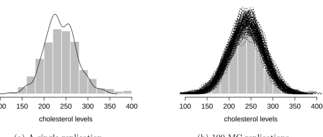
Figure (4.4a)represents a histogram of cholesterol levels of the 200 randomly

selected patients with the solid line as the fitted model under the proposed

set-tings. Moreover, figure (4.4b) shows the same histogram versus a 100 MC

repli-cations of bi.

cholesterol levels

100 150 200 250 300 350 400

cholesterol levels

100 150 200 250 300 350 400

(b) 100 MC replications

Figure 4.4: Fitting of Framingham Heart Study cholesterol data with model (4.3.2) using an exponential link and gamma distribution function, the shape parameter k= 3. The solid lines are the fitted model, while the histogram shows the frequency distribution of cholesterol levels.

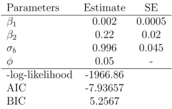
Similar to the simulation section above, table (4.4) presents the parameter

estimates and standard errors which are calculated as SE(θMLE) = √ 1

I(θMLE)

,

where I is the Fisher Information coefficient of the maximum likelihood estimate of parameter θ.

(63)

Table 4.4: Fitting of Framingham Heart Study cholesterol data with model (4.3.2) using an exponential link and gamma distribution function, the shape parameter

k = 3. Parameters Estimate SE β1 0.002 0.0005 β2 0.22 0.02 σb 0.996 0.045 φ 0.05 --log-likelihood -1966.86 AIC -7.93657 BIC 5.2567

Intuitively, one seeks comparison results with different models. As mentioned

earlier,Arellano-Valle et al.[2005] has fitted the Framingham Heart Study choles-terol data under a mixture of Gaussian and skew-normal distribution for the

random effects and residuals. The additive structure of the model is shown in

equation (4.3.1) with a bivariate random effect, while the presented model in

(4.3.2) uses one. For this reason, table (4.5) presents a numerical comparison

of average mean square error (Ave MSE) of two of Arellano-Valle et al. [2005]’s models to the presented copula-driven model, where the average is taken over

10000 runs.

A.V Model 1 A model with independent multivariate normal distribution for errors and multivariate skew-normal distribution for random effects with

λb = (λb1, λb2)

T_.

A.V Model 2 A model with independent multivariate skew-normal distribution for errors with common shape parameter between groups and multivariate

symmetric normal distribution for the random effects.

(64)

It is clear that the average MSE ofArellano-Valle et al.[2005] surpasses the fit of the proposed model; keep in mind, thatArellano-Valle et al.[2005] model have an extra random effect and parameters to estimate. Nevertheless, this is the first

step to estimate mixed models via a skew-normal copula, and future research is

inevitable for better fits, and most importantly, for the integration of a random

effects design matrix.

Table 4.5: Fitting of Framingham Heart Study cholesterol data comparison table with Arellano-Valle et al. [2005]

Factor A.V Model 1 A.V Model 2 Copula Driven-Model

(65)

Conclusion and final remarks

After characterizing the univariate and multivariate skew-normal distributions in

Chapter (1), we were able to use such findings to construct a skew-normal copula.

Chapter (2) works out all the details needed to simulate a general multivariate

distribution. Later chapters apply these findings to the exponential family

distri-bution, and present a complete derivation of the likelihood for a gamma and an

exponential distribution under different link functions. The numerical

approxi-mations and results in chapter (4.1) confirm the premise of this paper.

In future research, one can investigate different prior distribution functions

for thebi parameter in equation (3.2.4). For example, considering a skew-normal distribution for the random effects. Another possibility is to consider different

distributions for bi between units in longitudinal data, the possibility of such s