Negative Examples for Sequential Importance Sampling of
Binary Contingency Tables
Ivona Bez´akov´a∗ Alistair Sinclair† Daniel ˇStefankoviˇc‡ Eric Vigoda§
April 2, 2006
Keywords: Sequential Monte Carlo; Markov chain Monte Carlo; Graphs with prescribed degree sequence; Zero-one table
Abstract
The sequential importance sampling (SIS) algorithm has gained considerable popularity for its empirical success. One of its noted applications is to the binary contingency tables problem, an important problem in statistics, where the goal is to estimate the number of 0/1 matrices with prescribed row and column sums. We give a family of examples in which the SIS procedure, if run for any subexponential number of trials, will underestimate the number of tables by an exponential factor. This result holds for any of the usual design choices in the SIS algorithm, namely the ordering of the columns and rows. These are apparently the first theoretical results on the efficiency of the SIS algorithm for binary contingency tables. Finally, we present experimental evidence that the SIS algorithm is efficient for row and column sums that are regular. Our work is a first step in determining the class of inputs for which SIS is effective.
∗
Department of Computer Science, University of Chicago, Chicago, IL 60637. Email: [email protected].
†
Computer Science Division, University of California, Berkeley, CA 94720. Email: [email protected]. Supported by NSF grant CCR-0121555.
‡Department of Computer Science, University of Rochester, Rochester, NY 14627. Email: [email protected].
§College of Computing, Georgia Institute of Technology, Atlanta, GA 30332. Email:
[email protected]. Supported by NSF grant CCR-0455666.
1
Introduction
Sequential importance sampling is a widely-used approach for randomly sampling from complex distributions. It has been applied in a variety of fields, such as protein folding [6], population genetics [3], and signal processing [5]. Binary contingency tables is an application where the virtues of sequential importance sampling have been especially highlighted; see Chen et al. [2]. This is the subject of this note. Given a set of non-negative row sums r= (r1, . . . , rm) and column sums
c= (c1, . . . , cn), let Ω = Ωr,c denote the set ofm×n0/1 tables with row sums rand column sums
c. Our focus is on algorithms for sampling (almost) uniformly at random from Ω, or estimating|Ω|. Sequential importance sampling (SIS) has several purported advantages over the more classical Markov chain Monte Carlo (MCMC) method, such as:
Speed: Chen et al. [2] claim that SIS is faster than MCMC algorithms. However, we present a simple example where SIS requires exponential (in n, m) time. In contrast, a MCMC algorithm was presented in [4, 1] which is guaranteed to require at most time polynomial in n, m for every input.
Convergence Diagnostic: One of the difficulties in MCMC algorithms is determining when the Markov chain of interest has reached the stationary distribution, in the absence of analytical bounds on the mixing time. SIS seemingly avoids such complications since its output is guar-anteed to be an unbiased estimator of |Ω|. Unfortunately, it is unclear how many estimates from SIS are needed before we have a guaranteed close approximation of|Ω|. In our example for which SIS requires exponential time, the estimator appears to converge, but it converges to a quantity that is off from|Ω|by an exponential factor.
Before formally stating our results, we detail the sequential importance sampling approach for con-tingency tables, following [2]. The general importance sampling paradigm involves sampling from an ‘easy’ distribution µ over Ω that is, ideally, close to the uniform distribution. At every round, the algorithm outputs a tableT along withµ(T). Since for any µwhose support is Ω we have
we take many trials of the algorithm and output the average of 1/µ(T) as our estimate of|Ω|. More precisely, let T1, . . . ,Tt denote the outputs from ttrials of the SIS algorithm. Our final estimate is
Xt= 1 t X i 1 µ(Ti) . (1)
One typically uses a heuristic to determine how many trials t are needed until the estimator has converged to the desired quantity.
The sequential importance sampling algorithm of Chen et al. [2] constructs the table T in a column-by-column manner. It is not clear how to order the columns optimally, but this will not concern us as our negative results will hold for any ordering of the columns. Suppose the procedure is assigning column j. Let r0
1, . . . , rm0 denote the residual row sums after taking into account the
assignments in the firstj−1 columns.
The procedure of Chen et al. chooses column j from the correct probability distribution con-ditional on cj, r01, . . . , r0m and the number of columns remaining (but ignoring the column sums
cj+1, . . . , cn). This distribution is easy to describe in closed form. We assign column j the vector
(t1, . . . , tm)∈ {0,1}m,wherePiti =cj, with probability proportional to
Y i r0i n0−r0 i ti , (2)
where n0 = n−j+ 1. If no valid assignment is possible for the j-th column, then the procedure restarts from the beginning with the first column (and sets 1/µ(Ti) = 0 in (1) for this trial).
Sampling from the above distribution over assignments for column j can be done efficiently by dynamic programming.
Remark 1. Chen et al. devised a more subtle procedure which guarantees that there will always be a suitable assignment of every column. We do not describe this interesting modification of the procedure, as the two procedures are equivalent for the input instances which we discuss in this paper.
We now state our negative result. This is a simple family of examples where the SIS algorithm will grossly underestimate|Ω|unless the number of trials tis exponentially large. Our examples will have the form (1,1, . . . ,1, dr) for row sums and (1,1, . . . ,1, dc) for column sums, where the number
of rows is m+ 1, the number of columns isn+ 1, and we require that m+dr =n+dc.
Theorem 2. Let β > 0, γ ∈ (0,1) be constants satisfying β 6= γ and consider the input instances
r= (1,1, . . . ,1,bβmc), c = (1,1, . . . ,1,bγmc) withm+ 1 rows. Fix any order of columns (or rows, if sequential importance sampling constructs tables row-by-row) and let Xt be the random variable
representing the estimate of the SIS procedure after t trials of the algorithm. There exist constants
s1∈(0,1) and s2 >1 such that for every sufficiently large m and for any t≤sm2 ,
Pr Xt≥ |Ωr,c| sm 2 ≤3sm1 .
In contrast, note that there are MCMC algorithms which provably run in time polynomial in n and m for any row/column sums. In particular, the algorithm of Jerrum, Sinclair, and Vigoda [4] for the permanent of a non-negative matrix yields as a corollary a polynomial time algorithm for any row/column sums. More recently, Bez´akov´a, Bhatnagar and Vigoda [1] have presented a related sim-ulated annealing algorithm that works directly with binary contingency tables and has an improved polynomial running time. We note that, in addition to being formally asymptotically faster than any exponential time algorithm, a polynomial time algorithm has additional theoretical significance in that it (and its analysis) implies non-trivial insight into the the structure of the problem.
Some caveats are in order here. Firstly, the above results imply only that MCMC outperforms SIS asymptotically in the worst case; for many inputs, SIS may well be much more efficient. Secondly, the rigorous worst case upper bounds on the running time of the above MCMC algorithms are still far from practical. Chen et al. [2] showed several examples where SIS outperforms MCMC methods. We present a more systematic experimental study of the performance of SIS, focusing on examples where all the row and column sums are identical as well as on the “bad” examples from Theorem 2. Our experiments suggest that SIS is extremely fast on the balanced examples, while its performance on the bad examples confirms our theoretical analysis.
We begin in Section 2 by presenting a few basic lemmas that are used in the analysis of our negative example. In Section 3 we present our main example where SIS is off by an exponential factor, thus proving Theorem 2. Finally, in Section 4 we present some experimental results for SIS that support our theoretical analysis.
2
Preliminaries
We will continue to letµ(T) denote the probability that a tableT∈Ωr,c is generated by sequential importance sampling algorithm. We let π(T) denote the uniform distribution over Ω, which is the desired distribution.
Before beginning our main proofs we present two straightforward technical lemmas which are used at the end of the proof of the main theorem. The first lemma claims that if a large set of binary contingency tables gets a very small probability under SIS, then SIS is likely to output an estimate which is not much bigger than the size of the complement of this set, and hence very small. Let A= Ωr,c\A.
Lemma 3. Let p≤1/2and let A⊆Ωr,c be such that µ(A)≤p. Then for any a >1, and any t, we
have
Pr Xt≤aπ(A)|Ωr,c|
≥1−2pt−1/a.
Proof. The probability that all tSIS trials are not inA is at least
(1−p)t>exp(−2pt)≥1−2pt,
where the first inequality follows from ln(1−x) > −2x, valid for 0 < x ≤ 1/2, and the second inequality is the standard exp(−x)≥1−x forx≥0.
Let T1, . . . ,Tt be the t tables constructed by SIS. Then, with probability > 1−2pt, we have
Ti ∈A for all i. Notice that for a tableT constructed by SIS fromA, we have
E 1 µ(T) |T∈A =|A|.
LetF denote the event that Ti∈A for alli, 1≤i≤t; hence,
E(Xt| F) =|A|.
We can use Markov’s inequality to estimate the probability that SIS returns an answer which is more than a factor of a worse than the expected value, conditioned on the fact that no SIS trial is
from A:
Pr X > a|A| | F ≤ 1
a. Finally, removing the conditioning we get:
Pr(X≤a|A|) ≥ Pr X ≤a|A| | F Pr(F) ≥ 1− 1 a (1−2pt) ≥ 1−2pt−1 a.
The second technical lemma shows that if in a row with large sum (linear in m) there exists a large number of columns (again linear in m) for which the SIS probability of placing a 1 at the corresponding position differs significantly from the correct probability, then in any subexponential number of trials the SIS estimator will very likely exponentially underestimate the correct answer. Lemma 4. Let α < β be positive constants. Consider a class of instances of the binary contingency tables problem, parameterized by m, with m+ 1 row sums, the last of which is bβmc. LetAi denote
the set of all valid assignments of 0/1 to columns 1, . . . , i. Suppose that there exist constants f < g
and a setI of cardinality bαmc such that one of the following statements is true: (i) for every i∈I and any A∈ Ai−1,
π(Am+1,i = 1 |A)≤f < g≤µ(Am+1,i = 1 |A),
(ii) for every i∈I and any A∈ Ai−1,
µ(Am+1,i = 1 |A)≤f < g≤π(Am+1,i = 1 |A).
Then there exists a constantb1 ∈(0,1) such that for any constant 1< b2 <1/b1 and any sufficiently
large m, for any t≤bm
2 , Pr Xt≥ |Ωr,c| bm 2 ≤3(b1b2)m.
In words, in bm2 trials of sequential importance sampling, with probability at least 1−3(b1b2)m
the output is a number which is at most ab−2m fraction of the total number of corresponding binary contingency tables.
Proof. We will analyze case (i); the other case follows from analogous arguments. Consider indicator random variables Ui representing the event that the uniform distribution places 1 in the last row of
the i-th column. Similarly, let Vi be the corresponding indicator variable for the SIS. The random
variable Ui is dependent on Uj for j < i and Vi is dependent on Vj for j < i. However, each Ui
is stochastically dominated by U0
i which has value 1 with probability f, and each Vi stochastically
dominates the random variable V0
i which takes value 1 with probabilityg. Moreover, theUi0 andVi0
are respectively i.i.d.
Now we may use the Chernoff bound. Let k=bαmc. Then
Pr X i∈I Ui0−kf ≥ g−f 2 k ! <exp(−(g−f)2k/8) and Pr kg−X i∈I Vi0 ≥ g−f 2 k ! <exp(−(g−f)2k/8).
LetS be the set of all tables which have less thankf+ (g−f)k/2 =kg−(g−f)k/2 ones in the last row of the columns in I. Letb1 := exp(−(g−f)2α/16)∈(0,1). Then exp(−(g−f)2k/8)≤bm1 for
m≥1/α. Thus, by the first inequality, under uniform distribution over all binary contingency tables the probability of the set S is at least 1−bm
1 . However, by the second inequality, SIS constructs a
table from the setS with probability at mostbm
1 .
We are ready to use Lemma 3 with A = S and p = bm
1. Since under uniform distribution the
probability of S is at least 1−bm
1 , we have that |A| ≥ (1−bm1 )|Ωr,c|. Let b2 ∈ (1,1/b1) be any constant and consider t≤bm
2 SIS trials. Leta= (b1b2)−m. Then, by Lemma 3, with probability at
least 1−2pt−1/a≥1−3(b1b2)m the SIS procedure outputs a value which is at most anabm1 =b−2m
3
Proof of Main Theorem
In this section we prove Theorem 2. Before we analyze the input instances from Theorem 2, we first consider the following simpler class of inputs.
3.1 Row sums (1,1, . . . ,1, d) and column sums (1,1, . . . ,1)
The row sums are (1, . . . ,1, d) and the number of rows ism+ 1. The column sums are (1, . . . ,1) and the number of columns is n= m+d. We assume that sequential importance sampling constructs the tables column-by-column. Note that if SIS constructed the tables row-by-row, starting with the row with sum d, then it would in fact output the correct number of tables exactly. However, in the next subsection we will use this simplified case as a tool in our analysis of the input instances (1, . . . ,1, dr), (1, . . . ,1, dc), for which SIS must necessarily fail regardless of whether it works
row-by-row or column-by-column, and regardless of the order it chooses.
Lemma 5. Let β > 0, and consider an input of the form (1, . . . ,1,bβmc),(1, . . . ,1) with m+ 1
rows. Then there exist constants s1 ∈(0,1) and s2 >1, such that for any sufficiently large m, with
probability at least 1−3sm
1 , column-wise sequential importance sampling with sm2 trials outputs an
estimate which is at most a s−2m fraction of the total number of corresponding binary contingency tables. Formally, for any t≤sm
2 , Pr Xt≥ |Ωr,c| sm 2 ≤3sm1 .
The idea for the proof of the lemma is straightforward. By the symmetry of the column sums, for large m and d and α ∈ (0,1) a uniform random table will have about αd ones in the first αn cells of the last row, with high probability. We will show that for some α ∈ (0,1) and d = βm, sequential importance sampling is very unlikely to put this many ones in the firstαn columns of the last row. Therefore, since with high probability sequential importance sampling will not construct any table from a set that is a large fraction of all legal tables, it will likely drastically underestimate the number of tables.
distribution over all binary contingency tables with the SIS distributions. We refer to the column distributions induced by the uniform distribution over all tables as the truedistributions. The true probability of 1 in the first column and last row can be computed as the number of tables with 1 at this position divided by the total number of tables. For this particular sequence, the total number of tables is Z(m, d) = nd
m! = md+d
m!, since a table is uniquely specified by the positions of ones in the last row and the permutation matrix in the remaining rows and corresponding columns. Therefore, π(Am+1,1 = 1) = Z(m, d−1) Z(m, d) = m+d−1 d−1 m! m+d d m! = d m+d.
On the other hand, by the definition of sequential importance sampling, Pr(Ai,1= 1)∝ri/(n−ri),
whereri is the row sum in thei-th row. Therefore,
µ(Am+1,1 = 1) = d n−d d n−d+m 1 n−1 = d(m+d−1) d(m+d−1) +m2.
Observe that if d≈βm for some constant β >0, then for sufficiently largem we have
µ(Am+1,1= 1)> π(Am+1,1 = 1).
As we will see, this will be true for a linear number of columns, which turns out to be enough to prove that in polynomial time sequential importance sampling exponentially underestimates the total number of binary contingency tables with high probability.
Proof of Lemma 5. We will find a constant α such that for every column i < αm we will be able to derive an upper bound on the true probability and a lower bound on the SIS probability of 1 appearing at the (m+ 1, i) position.
For a partially filled table with columns 1, . . . , i−1 assigned, let di be the remaining sum in
the last row and let mi be the number of other rows with remaining row sum 1. Then the true
probability of 1 in thei-th column and last row can be bounded as
π(Am+1,i = 1 |A(m+1)×(i−1)) =
di
mi+di
≤ d
while the probability under SIS can be bounded as µ(Am+1,i= 1 |A(m+1)×(i−1)) = di(mi+di−1) di(mi+di−1) +m2i ≥ (d−i)(m+d−i−1) d(m+d−1) +m2 =:g(d, m, i).
Observe that for fixed m, d, the function f is increasing and the function g is decreasing in i, for i < d.
Recall that we are considering a family of input instances parameterized by m with d=dβme, for a fixedβ >0. We will consider i < αm for someα∈(0, β). Let
f∞(α, β) := lim m→∞f(d, m, αm) = β 1 +β−α; (3) g∞(α, β) := lim m→∞g(d, m, αm) = (β−α)(1 +β−α) β(1 +β) + 1 ; (4) 4β :=g∞(0, β)−f∞(0, β) = β2 (1 +β)(β(1 +β) + 1) >0, (5) and recall that for fixed β, f∞ is increasing in α and g∞ is decreasing in α, for α < β. Let α < β be such thatg∞(α, β)−f∞(α, β) =4
β/2. Such anα exists by continuity and the fact that
g∞(β, β) < f∞(β, β).
By the above, for any >0 and sufficiently largem, and for anyi < αm, the true probability is upper-bounded by f∞(α, β) +and the SIS probability is lower-bounded by g∞(α, β)−. For our purposes it is enough to fix = 4β/8. Now we can use Lemma 4 with α and β defined as above,
f = f∞(α, β) + and g = g∞(α, β)− (notice that all these constants depend only on β), and I ={1, . . . ,bαmc}. This finishes the proof of the lemma with s1=b1b2 and s2=b2.
Remark 6. Notice that every contingency table with row sums (1,1, . . . ,1, d) and column sums
(1,1, . . . ,1) is binary. Thus, this instance proves that the column-based SIS procedure for general (non-binary) contingency tables has the same flaw as the binary SIS procedure. We expect that the negative example used for Theorem 2 also extends to general (i. e., non-binary) contingency tables, but the analysis becomes more cumbersome.
3.2 Proof of Theorem 2
Recall that we are working with row sums (1,1, . . . ,1, dr), where the number of rows is m+ 1, and
column sums (1,1, . . . ,1, dc), where the number of columns is n+ 1 = m+ 1 +dr−dc. We will
eventually fixdr=bβmc anddc=bγmc, but to simplify our expressions we work withdr anddc for
now.
The theorem claims that the SIS procedure fails for an arbitrary order of columns with high probability. We first analyze the case when the SIS procedure starts with columns of sum 1; we shall address the issue of arbitrary column order later. As before, under the assumption that the first column has sum 1, we compute the probabilities of 1 being in the last row for uniform random tables and for SIS respectively. For the true probability, the total number of tables can be computed as
m dc n dr (m−dc)! + dcm−1 n dr−1
(m−dc+ 1)!, since a table is uniquely determined by the positions
of ones in the dc column anddr row and a permutation matrix on the remaining rows and columns.
Thus we have π(A(m+1),1) = m dc n−1 dr−1 (m−dc)! + dcm−1 n−1 dr−2 (m−dc+ 1)! m dc n dr (m−dc)! + dcm−1 n dr−1 (m−dc+ 1)! = dr(n−dr+ 1) +dcdr(dr−1) n(n−dr+ 1) +ndcdr =:f2(m, dr, dc); µ(A(m+1),1) = dr n−dr dr n−dr +m 1 n−1 = dr(n−1) dr(n−1) +m(n−dr) =:g2(m, dr, dc).
Letdr=bβmcanddc =bγmcfor some constantsβ >0, γ ∈(0,1) (notice that this choice guarantees
thatn≥dr and m≥dc, as required). Then, asm tends to infinity,f2 approaches
f2∞(β, γ) := β 1 +β−γ, and g2 approaches g2∞(β, γ) := β(1 +β−γ) β(1 +β−γ) + 1−γ. Notice that f∞
2 (β, γ) = g2∞(β, γ) if and only if β = γ. Suppose that f2∞(β, γ) < g∞2 (β, γ) (the
of Lemma 5, we can defineαsuch that if the importance sampling does not choose the column with sum dc in its first αm choices, then in any subexponential number of trials it will exponentially
underestimate the total number of tables with high probability. Formally, we derive an upper bound on the true probability of 1 being in the last row of thei-th column, and a lower bound on the SIS probability of the same event (both conditioned on the fact that the dc column is not among the
firsticolumns assigned). Let d(ri) be the current residual sum in the last row,mi be the number of
rows with sum 1, andni the remaining number of columns with sum 1. Notice thatni =n−i+ 1,
m≥mi≥m−i+ 1, anddr≥d(ri) ≥dr−i+ 1. Then π(A(m+1),i |A(m+1)×(i−1)) = d(ri)(ni−d(ri)+ 1) +dcd(ri)(d(ri)−1) ni(ni−dr(i)+ 1) +nidcd(ri) ≤ dr(n−dr+ 1) +dcd 2 r (n−i)(n−i−dr) + (n−i)dc(dr−i) =:f3(m, dr, dc, i); µ(A(m+1),i |A(m+1)×(i−1)) = d (i) r (ni−1) d(ri)(ni−1) +mi(ni−d(ri)) ≥ (dr−i)(n−i) drn+m(n−dr) =:g3(m, dr, dc, i).
As before, notice that if we fix m, dr, dc >0 satisfying dc < m and dr< n, then f3 is an increasing
function andg3 is a decreasing function in i, fori < min{n−dr, dr}. Recall that n−dr =m−dc.
Suppose that i ≤ αm < min{m−dc, dr} for some α which we specify shortly. Thus, the upper
bound onf3 in this range ofiis f3(m, dr, dc, αm) and the lower bound on g3 isg3(m, dr, dc, αm). If
dr =bβmc anddc =bγmc, then the upper bound on f3 converges to
f3∞(α, β, γ) := lim
m→∞f3(m, dr, dc, αm) =
β2
(1 +β−γ −α)(β−α) and the lower bound on g3 converges to
g∞3 (α, β, γ) := lim
m→∞g3(m, dr, dc, αm) =
(β−α)(1 +β−γ−α) β(1 +β−γ) + 1−γ
Let
4β,γ :=g3∞(0, β, γ)−f3∞(0, β, γ) =g2∞(β, γ)−f2∞(β, γ)>0.
We setα to satisfyg∞
3 (α, β, γ)−f3∞(α, β, γ) ≥ 4β,γ/2 andα <min{1−γ, β}. Now we can conclude
this part of the proof identically to the last paragraph of the proof of Lemma 5.
It remains to deal with the case when sequential importance sampling picks thedc column within
the first bαmc columns. Suppose dc appears as the k-th column. In this case we focus on the
subtable consisting of the lastn+ 1−kcolumns with sum 1, m0 rows with sum 1, and one row with sumd0, an instance of the form (1,1, . . . ,1, d0),(1, . . . ,1). We will use arguments similar to the proof of Lemma 5.
First we express d0 as a function ofm0. We have the bounds (1−α)m≤m0 ≤m and d−αm≤ d0 ≤dwhere d=bβmc ≥βm−1. Let d0 =β0m0. Thus,β−α−1/m≤β0 ≤β/(1−α).
Now we findα0 such that for anyi≤α0m0 we will be able to derive an upper bound on the true probability and a lower bound on the SIS probability of 1 appearing at position (m0 + 1, i) of the (n+ 1−k)×m0 subtable, no matter how the firstk columns were assigned. In order to do this, we might need to decrease α – recall that we are free to do so as long as α is a constant independent of m. By the derivation in the proof of Lemma 5 (see expressions (3) and (4)), as m0 (and thus also m) tends to infinity, the upper bound on the true probability approaches
f∞(α0, β0) = lim m→∞ β0 1 +β0−α0 ≤mlim→∞ β 1−α 1 +β−α−m1 −α0 = β 1−α 1 +β−α−α0 =:f ∞ 4 (α, β, α0)
and the lower bound on the SIS probability approaches
g∞(α0, β0) = lim m→∞ (β0−α0)(1 +β0−α0) β0(1 +β0) + 1 ≥mlim→∞ (β−α−m1 −α0)(1 +β−α− 1 m −α 0) β 1−α(1 + β 1−α) + 1 = (β−α−α 0)(1 +β−α−α0) β 1−α(1 + β 1−α) + 1 ≥ (β−α−α 0)(1 +β−α−α0) β 1−α(1−1α + β 1−α) +(1−1α)2 =:g4∞(α, β, α0), where the last inequality holds as long asα <1. Notice that for fixedα, β satisfying α <min{1, β}, the function f∞
4 is increasing and g∞4 is decreasing in α0, forα0 < β−α. Similarly, for fixed α0, β
satisfying α0 < β, the function f∞
Therefore, if we takeα=α0 <min{1, β/2}, we will have the bounds
f4∞(x, β, y)≤f4∞(α, β, α) and g4∞(x, β, y)≥g4∞(α, β, α) for any x, y≤α.
Recall that 4β = g∞(0, β) −f∞(0, β) = g4∞(0, β,0)−f4∞(0, β,0) > 0. If we choose α so that
g∞
4 (α, β, α) −f4∞(α, β, α) ≥ 4β/2, then in similar fashion to the last paragraph of the proof of
Lemma 5, we may conclude that the SIS procedure likely fails. More precisely, let:=4β/8 and let
f := f∞
4 (α, β, α) + and g := g4∞(α, β, α)−be the upper bound (for sufficiently large m) on the
true probability and the lower bound on the SIS probability of 1 appearing at the position (m+ 1, i) for i ∈ I := {k+ 1, . . . , k+bα0m0c}. Therefore Lemma 4 with parameters α(1−α), β, I of size |I|=bα0m0c ≥ bα(1−α)mc,f, and gimplies the statement of the theorem.
Finally, if the SIS procedure constructs the tables row-by-row instead of column-by-column, symmetrical arguments hold. This completes the proof of Theorem 2.
2
4
Experiments
We performed several experimental tests which show sequential importance sampling to be a promis-ing approach for certain classes of input instances.
We ran sequential importance sampling algorithm for binary contingency tables, using the fol-lowing stopping heuristic. Let N =n+m. For some , k >0 we stopped if the last kN estimates were all within a (1 +) factor of the current estimate. We set = 0.01 and k= 5.
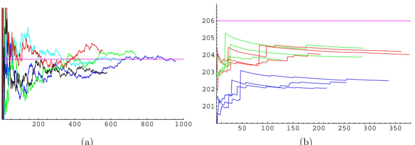
Figure 1(a) shows the evolution of the SIS estimate as a function of the number of trials on the input with all row and column sums ri =cj = 5, and 50×50 matrices. In our simulations we used
the more delicate sampling mentioned in Remark 1, which guarantees that the assignment in every column is valid, i. e., such an assignment can always be extended to a valid table (or, equivalently, that the random variableXtis always strictly positive). Five independent runs are depicted, together
with the correct number of tables ≈1.038×10281, which we computed exactly. To make the figure
that the algorithm appears to converge to the correct estimate, and our stopping heuristic appears to capture this behavior.
In contrast, Figure 1(b) depicts the SIS evolution on the negative example from Theorem 2 with m= 300, β = 0.6 and γ = 0.8, i. e., the input is (1, . . . ,1,179),(1, . . . ,1,240) on a 301×240 matrix. In this case the correct number of tables is
300 240 239 179 (300−240)! + 300 239 239 178 (300−239)!≈9.684×10205.
We ran the SIS algorithm under three different settings: first, we constructed the tables column-by-column where the column-by-columns were ordered from the largest sum, as suggested in the paper by Chen et al. [2] (the red curves correspond to three independent runs with this setting); second, we ordered the columns from the smallest sum (the green curves); and third, we constructed the tables row-by-row where the rows were ordered from the largest sum (the blue curves). The y-axis is on a logarithmic scale (base 10) and one unit on thex-axis corresponds to 1000 SIS trials. We ran the SIS estimates for twice the number of trials determined by our stopping heuristic to indicate that the unfavorable performance of the SIS estimator on this example is not the result of a poor choice of stopping heuristic. Notice that even the best estimator differs from the true value by about a factor of 40, while the blue curves are off by more than a factor of 1000.
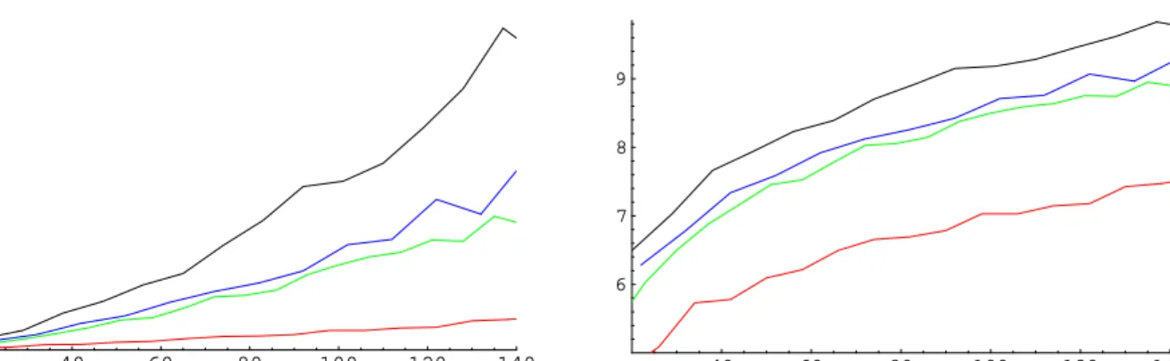
Figure 2 represents the number of trials required by the SIS procedure (computed by our stopping heuristic) on several examples forn×nmatrices. The four curves correspond to 5, 10,b5 lognc and bn/2c-regular row and column sums. Thex-axis representsn, the number of rows and columns, and they-axis captures the required number of SIS trials. For eachnand each of these row and column sums, we took 20 independent runs and we plotted the median number of trials. For comparison, in Figure 3 we plotted the estimated running time for our bad example from Theorem 2 (recall that this is likely the running time needed to converge to a wrong value!) for n+m ranging from 20 to 140 and various settings of β, γ: 0.1,0.5 (red), 0.5,0.5 (blue), 0.2,0.8 (green), and 0.6,0.8 (black). In this case it is clear that the convergence time is considerably slower compared with the examples in Figure 2.
References
[1] I. Bez´akov´a, N. Bhatnagar, and E. Vigoda, Sampling Binary Contingency Tables with a Greedy Start. In Proceedings of the 17th Annual ACM-SIAM Symposium on Discrete Algo-rithms(SODA), 2006.
[2] Y. Chen, P. Diaconis, S. Holmes, and J.S. Liu, Sequential Monte Carlo Methods for Statistical Analysis of Tables.Journal of the American Statistical Association, 100:109-120, 2005.
[3] M. De Iorio, R. C. Griffiths, R. Lebois, and F. Rousset, Stepwise Mutation Likelihood Com-putation by Sequential Importance Sampling in Subdivided Population Models. Theor. Popul. Biol., 68:41-53, 2005.
[4] M.R. Jerrum, A. Sinclair and E. Vigoda, A Polynomial-time Approximation Algorithm for the Permanent of a Matrix with Non-negative Entries. Journal of the Association for Computing Machinery, 51(4):671-697, 2004.
[5] J. Miguez and P. M. Djuric, Blind Equalization by Sequential Importance Sampling.Proceedings of the IEEE International Symposium on Circuits and Systems, 845-848, 2002.
[6] J. L. Zhang and J. S. Liu, A New Sequential Importance Sampling Method and its Application to the Two-dimensional Hydrophobic-Hydrophilic Model.J. Chem. Phys., 117:3492-8, 2002.
200 400 600 800 1000 10.1 10.2 10.3 10.4 10.5 10.6 (a) 50 100 150 200 250 300 350 201 202 203 204 205 206 (b)
Figure 1: The estimate produced by sequential importance sampling as a function of the number of trials on two different instances. In both figures, the horizontal line shows the correct number of corresponding binary contingency tables. (a) The left instance is a 50×50 matrix where all ri = cj = 5. The x-axis is the number of SIS trials, and the y-axis corresponds to the estimate
scaled down by a factor of 10280. Five independent runs of sequential importance sampling are depicted. Notice that the y-axis ranges from 10 to 10.7, a relatively small interval, thus it appears SIS converges to the correct estimate. (b) The input instance is from Theorem 2 with m = 300, β = 0.6 and γ = 0.7. The estimate (y-axis) is plotted on a logarithmic scale (base 10) and one unit on thex-axis corresponds to 1000 SIS trials. Note that in this instance SIS appears to converge to an incorrect estimate. Nine independent runs of the SIS algorithm are shown: the red curves construct tables column-by-column with columns sorted by decreasing sum, the blue curves construct row-by-row with row-by-rows sorted by decreasing sum, and the green curves construct column-by-column with columns sorted increasingly.
20 40 60 80 100 200 400 600 800 1000 1200
Figure 2: The number of SIS trials before the algorithm converges, as a function of the input size. The curves correspond to 5 (red), 10 (blue), b5 lognc (green), and bn/2c (black) regular row and column sums.
40 60 80 100 120 140 2500 5000 7500 10000 12500 15000 17500 40 60 80 100 120 140 6 7 8 9
Figure 3: The number of SIS trials until the algorithm converges as a function of m+n. The inputs are of the type described in Theorem 2, with β = 0.1, γ = 0.5 (red), β = γ = 0.5 (blue), β = 0.2, γ = 0.8 (green), and β = 0.6, γ = 0.8 (black). The right plot shows the same four curves with the number of SIS trials plotted on a logarithmic scale. Note that the algorithm appears to be converging in sub-exponential time. Recall from Figure 1 that it is converging to the wrong estimate.