Dynamical response to the solar cycle
Kunihiko Kodera and Yuhji Kuroda
Meteorological Research Institute, Tsukuba, Japan
Received 22 February 2002; revised 3 July 2002; accepted 15 August 2002; published 19 December 2002.
[1] The dynamical impact of the 11-year solar cycle is investigated with the focus on the stratopause region where solar ultraviolet heating is greatest. The most important
variation in solar forcing longer than the diurnal cycle is the annual cycle. Thus the climatological features of the zonal wind variation associated with the annual cycle were first studied to characterize the basic features of the atmosphere’s dynamical response to changes in solar radiative forcing. The 11-year solar cycle effect was then investigated. The results of the analysis suggest that in a climatological mean state the stratopause circulation evolves from a radiatively controlled state to one dynamically controlled during winter in both hemispheres. The transition period is characterized by a poleward shift of the westerly jet. The solar cycle effect appears as a change in the balance between the radiatively and dynamically controlled states. The radiatively controlled state lasts longer during the solar maximum phase, and the stratopause subtropical jet reaches a higher speed. The large dynamical response to relatively weak radiative forcing may be understood by the bimodal nature of the winter atmosphere due to interaction with meridionaly propagating planetary waves and zonal mean zonal winds. It is suggested that the solar influence produced in the upper stratosphere and stratopause region is transmitted to the lower stratosphere through (1) modulation of the internal mode of variation in the polar night jet and (2) a change in the Brewer-Dobson circulation. The first process is significant in the middle and high latitudes, whereas the latter is prominent in the equatorial region. INDEXTERMS:1650 Global Change: Solar variability; 3309 Meteorology and Atmospheric Dynamics: Climatology (1620); 3319 Meteorology and Atmospheric Dynamics: General circulation; 3334 Meteorology and Atmospheric Dynamics: Middle atmosphere dynamics (0341, 0342); KEYWORDS:solar influence, solar cycle, middle atmosphere dynamics, stratosphere
Citation: Kodera, K., and Y. Kuroda, Dynamical response to the solar cycle,J. Geophys. Res.,107(D24), 4749, doi:10.1029/ 2002JD002224, 2002.
1. Introduction
[2] It is well known that the activity of the Sun changes with a periodicity of approximately eleven years. However, it has long been a matter of debate whether the 11-year solar cycle has any significant effect on Earth’s surface climate [e.g.,Pittock, 1978].
[3] The absorption of solar irradiance creates two warm regions in the atmosphere, one near Earth’s surface and the other at the stratopause; the higher temperature near the surface is due to the absorption of visible light, while that in the stratopause region is due to the absorption of solar ultraviolet (UV) light by the ozone. Recent measurements from space indicate that the total solar irradiance changes associated with the 11-year solar cycle are negligibly small (0.1%), although larger (4 – 8%) variations are found in the ultraviolet (UV) range of 200 – 250 nm [Lean et al., 1997]. Even if we do not expect direct solar cycle impacts at Earth’s surface, a significant influence should be detected in the stratopause region.
[4] Observational studies indicate an ozone increase of about 3 – 5% and a temperature change of 1K in the upper stratosphere during a solar cycle [Hood et al., 1993; McCor-mack and Hood, 1996; Stratospheric Processes and Their Role in Climate(SPARC), 1998]. An enhanced meridional temperature gradient between the equatorial and polar regions could produce stronger zonal winds during winter [Kodera and Yamazaki, 1990]. It has been suggested [Kodera et al, 1990; Kodera, 1995] that the zonal mean zonal wind anomalies formed in the upper stratosphere and stratopause region in early winter can propagate downward into the troposphere through dynamical processes. However, the lack of a homogeneous long-term global dataset makes it difficult to obtain reliable evidence from observations.
[5] The impact of the solar UV heating changes has been tested using general circulation models (GCMs) [Balachan-dran and Rind, 1995;Rind and Balachandran, 1995]. Recent middle atmosphere GCM simulations using an observed solar energy spectrum and the associated ozone changes of the solar cycle produced measurable effects in the tropo-sphere [Haigh, 1999;Shindell et al., 1999, 2001]. However, it is difficult to properly evaluate such complex model results without knowing the responsible mechanism. The aim of this
Copyright 2002 by the American Geophysical Union. 0148-0227/02/2002JD002224$09.00
study is not to demonstrate the solar influence itself but to obtain insight into a possible mechanism that can be tested later with numerical model simulations.
[6] While the present study focuses on solar cycle effects, it should be noted that the most important variability in solar radiative forcing longer than the diurnal cycle, is the annual cycle and is produced by changes in the solar zenith angle due to the rotation of Earth around the Sun. Eleven-year solar cycle variations of solar activity should then appear in the first approximation as small amplitude modulations of the annual cycle. Solar radiative heating due to the absorp-tion of solar UV through ozone in the upper stratosphere and stratopause regions creates a large temperature gradient during winter, which consequently induces a strong west-erly jet. However, the zonal wind velocity is not simply dependent on radiative forcing alone but is determined through interaction with atmospheric waves propagating up to the stratosphere and mesosphere. Both the essential role of planetary waves in creating the seasonal cycle and the differences between the Southern Hemisphere (SH) and Northern Hemisphere (NH) [Hirota et al., 1983] are well depicted in simple mechanistic models [Plumb, 1989; Yoden, 1990].
[7] Solar cycle effects are usually investigated in terms of anomalies from a climatology or differences between max-imum and minmax-imum phases. The dynamical response in the winter stratosphere includes the highly nonlinear processes of wave mean flow interactions, so both the anomalies and the total field including the climatological states, must be taken into account. Therefore we first studied the climato-logical features of the zonal wind variations associated with the annual cycle to characterize the basic features of the atmospheric dynamical response to changes in solar radia-tive forcing. It is also necessary to study the nature of interannual variability since substantial year-to-year varia-tions exist. Finally, the 11-year solar cycle effect was investigated by comparing its effects with those related to the annual cycle.
[8] Observational studies [see van Loon and Labitzke, 2000] indicate a large solar influence in the lower strato-sphere. It is particularly clear during the NH winter when winter is separated according to the phase of the equatorial QBO [Labitzke, 1987;Labitzke and van Loon, 1988]. In this paper, however, we first focus on the stratopause region where the solar UV impact is expected to be greater and more direct than elsewhere in the middle atmosphere, and then the problem of downward penetration of solar influ-ences is investigated.
[9] The possibility of producing tropospheric effects through changes in vertical propagation of planetary waves due to the stratospheric zonal wind variation induced by the solar cycle has been investigated using linear models. This direct influence of a zonal wind change is negligibly small if the wind change does not occur in sufficiently low altitudes [Geller and Alpert, 1980]. However, the zonal wind anoma-lies produced in the upper stratosphere can propagate downward into the troposphere when the interaction between the zonal flow and waves is included [Kodera et al., 1990; Christiansen, 2001]. Another possibility is that modification of the wave mean flow interaction in the upper level drives changes in meridional circulation down to the surface, which is known as the ‘‘downward control
princi-ple’’ [Haynes et al., 1991]. Both processes involve a wave mean flow interaction.
[10] This paper is organized as follows. Section 2 explains the data used and related problems. The results of analysis on the annual cycle, interannual variability, influence of the solar cycle at the stratopause region and the downward extension are described in section 3. After the discussion in section 4, concluding remarks are given in section 5.
2. Data
[11] The dataset used in the present study is the same as the one used byKuroda and Kodera[2001], except for the 0.4 hPa level data that are included here. Balanced winds in the stratosphere are calculated from the geopotential height data analyzed from the National Centers for Environmental Prediction (NCEP), formerly the National Meteorological Center (NMC) [Randel, 1992]. The reanalysis data from NCEP [Kalnay et al., 1996] are used below 100 hPa. Pentad (5-day) mean data are created as a basic dataset for the period 1979 – 1998 after all missing data are interpolated. The monthly mean data are then calculated by averaging the pentad data. Similarly, the monthly mean Eliassen-Palm (E-P) flux data are based on the E-P flux calculated from the pentad data.
[12] Residual circulation is calculated by iteratively solv-ing the transformed Eulerian momentum equation (1) and continuity equation (2), as bySoel and Yamazaki[1999]. utþv*½ðacosfÞ 1 ucosf ð Þff þw*uzþX ¼ðr0acosfÞ 1 divF ð1Þ acosf ð Þ1ðv* cosfÞfþr 1 0 ðr0w*Þz¼0 ð2Þ
All variables here are the zonal mean. The notation of the equations followsAndrews et al.[1987].
[13] The quality of the NCEP data is poor until the middle of the 1980s. It is not always possible to obtain reasonable values in the lower latitudes. One method is to use only recent periods, as bySoel and Yamazaki [1999]. However, at least two solar cycles are needed to distinguish a solar cycle variation from a long-term trend. Therefore we used the whole period of available data from 1979 through 1998 for our analysis. As a result, a quantitative estimate of the residual circulation in the low latitudes becomes difficult. Therefore only a qualitative discussion is offered. Another problem for the present period of analysis, 1979 – 1998, is that two large volcanic eruptions occurred in the lower latitudes near the solar maxima, one in 1982 (El Chichon) and the other in 1991 (Pinatubo), which strongly disturbed the lower tropical stratosphere. Distinguishing solar influ-ence from volcanic eruption is consequently difficult for this limited period, particularly in the equatorial lower strato-sphere [Solomon et al., 1996].
3. Results 3.1. Annual Cycle
[14] A 20-year climatology profile (data from January 1979 to December 1998) was constructed to study the mean
annual cycle. Figure 1 shows the climatological monthly mean zonal mean zonal winds during the cold season from May to September in the Southern Hemisphere, SH (left), and from November to March in the Northern Hemisphere, NH (right). The zonal winds in the subtropical stratopause in the SH increase from autumn and attained maximum values in June; the core of the westerly jet shifts gradually poleward during winter. An additional downward move-ment of the jet from the lower mesosphere to the lower stratosphere was identified. The origin of the annual cycle is the rotation of Earth around the Sun. Therefore variations gradually occur in radiative forcing. A rapid variation during the seasonal march should be the result of dynamical forcing, and the result of changes in wave forcing in particular. The dynamical contribution to the seasonal march is therefore more clearly depicted in the high-pass filtered climatological data, calculated as the deviation from the three-month running mean (Figure 2). A poleward and downward propagation of the anomalies from the equatorial lower mesosphere to the lower stratosphere can clearly be seen. A similar poleward and downward movement of the zonal wind anomalies can be traced in the high-pass filtered data in the NH, although it is not very easily seen in the total field (Figure 1). However, the poleward movement is more rapid in the NH (it has already terminated in January) than in the SH, where it finishes in September.
[15] It is evident from Figure 2 that the seasonal march of the zonal winds is characterized well by the winds around the stratopause region. The zonal winds in the subtropical stratopause are connected to the lower meso-sphere in early winter, while those at high latitudes are connected to the polar-night jet of the middle and lower stratosphere during late winter. Zonal winds in the sub-tropical and the high latitude stratopause were chosen in the present study as representative of the seasonal cycle and solar cycle effects and will be analyzed in detail. Shiotani et al. [1993] used zonal winds at 30S and 60S latitudes to analyze the stratopause jet variation in the SH. The analysis of Kuroda and Kodera [2001] reveals a seesaw in the zonal mean zonal winds between around 35S and 65S. Therefore zonal mean zonal winds at 35
and 60 near the stratopause (at 1 hPa) were chosen to characterize variations in the subtropical jet (SJ) and the polar night jet (PJ). The result is not sensitive to the small difference in the selected latitudes.
[16] Figure 3a shows a time series of the climatological fifteen-day running mean zonal mean zonal wind at 1 hPa during the cold season in the SH (left) and the NH (right). The climatology was calculated from 19 winters in which December and January belong to the same winter, for better continuity during the NH winter. The thick and thin lines represent the zonal winds at 35and 60. The present study uses five-day mean data, and the 35th and 72nd pentads are treated as solstices. The SJ and the PJ increase from autumn (April/May) to early winter (May/June) in the SH. The increase of the PJ is interrupted in May, whereas the SJ grows monotonically until it reaches the maximum velocity in mid-June. The PJ resumes increasing when the SJ starts decreasing. The increase of the PJ stops in August, and it rapidly decreases from September on.
[17] The periods in which the weakening of the SJ occurs in association with the strengthening of the PJ
Figure 1. Climatological monthly mean zonal mean zonal winds during the cold season. (left) May through September in the SH from 20S to 80S. (right) November through March in the NH from 20N to 80N. Contour interval is 10 ms1and negative values are shaded.
correspond to a poleward jet shift (indicated by closed circles). The periods of rapid weakening of the PJ (the weakening tendency of the PJ is 1.3 times more rapid than that of the SJ, indicated by open circles in Figure 3b) correspond to a rapid increase of polar temperatures in the middle stratosphere at 30 hPa. The period of time with a decreasing SJ (closed circles in Figure 3b) has no clear correspondence with polar temperatures, except for some slowing down of cooling. A similar seasonal march is recognized in the NH until a rapid decrease of the PJ in January, despite the more irregular variation in the PJ that reflects the occurrence of large midwinter warmings. The decrease of the SJ in the SH occurs in mid-June, near the winter solstice, whereas it occurs in November in the NH, about one month earlier than the winter solstice. The SJ does not decrease monotonically in the NH, but shows a small increase before weakening in the spring. The warm-ing in midwinter (January) also starts earlier in the NH, whereas it occurs at the approach of the vernal equinox (September) in the SH.
[18] The evolution of the SJ and PJ can be characterized more clearly as a trajectory in a plane spanned by the SJ (ordinate) and the PJ (abscissa) (Figure 4). Fifteen-day running mean data were plotted every five days for the period shown in Figure 3. The decreasing period of the SJ in association with an increase of the PJ is indicated by closed and the rapid decreasing periods of the PJ are indicated by open circles in Figure 4, similar to Figure 3. The trajectories of both hemispheres exhibit a similar structure, although the beginning of the warming (open circles) is not well marked in the SH, whereas the start of the jet shift (closed circles) is less clear in the NH. It should also be noted that the evolution speed in the NH is more rapid and the amplitude of the wind speed is smaller than in the SH. Despite the many differences between the SH and the NH circulation [Hirota et al., 1983], the seasonal march during the cold season can be commonly characterized by three stages or phases:
I. Monotonic increase of the SJ
II. From a decrease of the SJ and a simultaneously increase of the PJ to a rapid decrease of the PJ
III. Following the rapid decrease of the PJ
These three phases are indicated in Figures 3 and 4 by Roman numerals.
3.2. Interannual Variability
[19] The annual cycle of the stratopause jet described above is the mean feature obtained by averaging 19 winters. The observed circulation differs significantly from one year to another. Such interannual variability is considered to arise primarily from the difference in wave forcing. The inter-annual variability in the present section is investigated based on the monthly mean data. The top panels of Figures 5a and 5b illustrate the evolution of the SJ and the PJ for 19 individual winters. The bar graphs in the panels below depict the standard deviations from the 19-winter mean. The three phases of the seasonal march based on the climatological data in Figure 3 are also indicated in Figure 5 to illustrate the differences in the interannual variability according to the different stages of the seasonal march. We make use here of the monthly mean data, and therefore the Figure 2. Same as Figure 1, but for high-pass filtered
climatological monthly mean zonal mean zonal winds. Contour interval is 2 ms1.
three phases of the climatological seasonal march are defined as follows:
SH: I) April, May; II) Jun, July, August; III) September NH: I) October; II) November, December; III) January, February, March
[20] The interannual variability of the SJ (Figure 5a) is very small during climatological phase I. The variability becomes very large during climatological phase II and decreases again during climatological phase III. The inter-annual variability of the PJ (Figure 5b) increases with time and the greatest variability appears in phase III. These findings are true for both hemispheres. It is interesting to note that the variability of the SJ in the SH is as large as in
the NH, whereas the interannual variability of the PJ in the SH is substantially smaller than that in the NH. The large variability of the SJ in the SH during climatological phase II seems to be associated with the variation in the start of the decreasing period; in some years the SJ starts to decrease rapidly beginning in June, but in other years the SJ decreases slowly with time. The SJ generally decreases from November in the NH, but for a few years it continued to increase until December. This suggests that the large interannual variation in the SJ arises from the advance or the delay of the seasonal march.
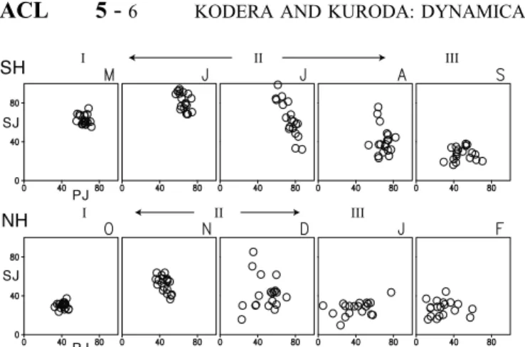
[21] Scatter diagrams of the SJ and PJ for all 20 years are plotted for each month in Figure 6 to illustrate the character-istic features of their seasonal variations and their interre-lationships. The top panels depict the SH from May through September, and the bottom panels show NH from October through February. The ordinate indicates the SJ velocities, and the abscissa those of the PJ. The three climatological phases of the seasonal march are also shown in Figure 6. The interannual variation is very small during climatolog-ical phase I, and the points are distributed around a climatological mean value. All points are distributed along an inclined line from the upper left to the lower right in the early part of climatological phase II, indicating a seesaw between SJ and the PJ. The SJ/PJ seesaw is recognized in the latter part (August in the SH and December in the NH) only when the SJ is sufficiently strong (>35 ms1). They are distributed along a line inclined in the opposite direction (from the lower left to the upper right) when the SJ is weak, indicating simultaneous strengthening and weakening of the SJ and the PJ. The SJ is weak during climatological phase III, and variability is mainly seen in the PJ, which is distributed along a horizontal line. To summarize, the points in the scatter diagrams are distributed roughly parallel to the Figure 3. (a) Time series of the climatological fifteen-day
mean zonal mean zonal winds at 1 hPa at 35 (thick line) and 60 (thin line) latitudes during 180 days around the winter solstice. Left and right panels show the SH and NH, respectively. (b) Same as Figure 3a, but for the polar temperature at 30 hPa. Closed and open circles correspond to periods of a jet shift and warmings, respectively, which characterize the three winter phases indicated by dashed lines and Roman numerals (I – III).
Figure 4. Phase diagram of SJ (ordinate) and PJ (abscissa) during the cold season displayed in Figure 3. Closed and open circles correspond to periods of a jet shift and warmings, respectively. The numbers indicate the three phases, similar to Figure 3.
Figure 5. (a) (top) Monthly mean zonal mean SJ (zonal winds at 1 hPa, 35 latitudes) for 19 winters. (bottom) Standard deviation from the19-year mean. (b) Same as Figure 5a but for PJ (zonal winds at 1 hPa, 60 latitudes). Dashed lines indicate the three climatological phases of the seasonal march.
trajectory of the climatological seasonal march displayed in Figure 4 during climatological phases II and III. This suggests that the substantial interannual variability of the individual months is caused by the changing evolution speed of the seasonal march.
[22] The direct cause of the large interannual variation of the zonal mean zonal winds should be an in situ wave
forcing. Figure 7 shows scatter diagrams of the SJ (zonal mean zonal wind at 35, 1hPa); (a) is the horizontal and (b) the vertical components of the E-P flux at 45latitudes and 1 hPa. All variables are standardized in the diagrams. The variation of strength in the SJ is highly correlated with the horizontal component of the E-P flux in both hemispheres, shown in Figure 7a at0.87 in the SH (left) and 0.91 in the NH (right). The correlation with the vertical component is high (0.79) in the SH but only marginally significant (0.43) in the NH (Figure 7b). This indicates that the variation of the SJ is more closely related to a change in the meridional propagation of waves than to a change in the vertical propagation.
3.3. Solar Cycle
[23] The solar cycle effects will be investigated in this section and compared to the annual cycle. The 11-year solar cycle is depicted in Figure 8 with a time series of the monthly mean 10.7 cm solar radio flux as a measure of the solar activity. The present analysis period from 1979 – 1998 covers only two solar cycles (21 and 22). The solar maximum and minimum phases are defined with equal periods of four years to simplify further analyses: the solar max (cycle 21) from 1979 – 1982, solar minimum from 1984 – 1987; solar maximum (cycle 22) from 1988 – 1991, solar minimum from 1994 – 1997. The composite means for the solar maximum and minimum phases are calculated for years in which June (SH) or December (NH) falls into the above list.
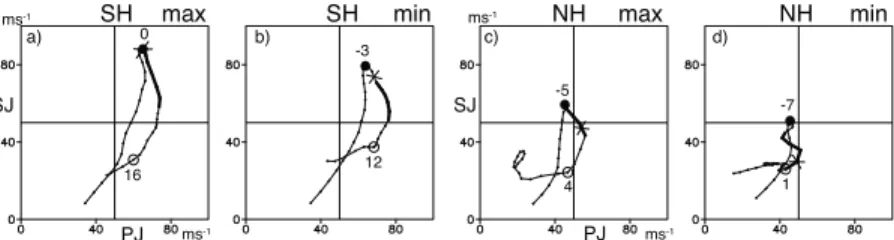
[24] Figure 9 shows the same phase diagram of the SJ and PJ as in Figure 4, but now separated for an eight-year composite mean during solar maximum and minimum phases. The closed- and open circles indicate the starting periods of climatological phases II and III, respectively, defined according to the same criterion used in Figure 4. Crosses indicate winter solstices. The start of phase II coincides with the winter solstice during solar maximum in the SH, whereas it starts 15 days earlier for the solar minimum. Similarly, the start of phase III occurs 20 days later for the solar maximum than for the minimum. Phase II (III) start ten days (fifteen days) later in the NH during solar maximum compared to solar minimum. The numbers in the figure indicate the starting time in the pentad of phases II and III from the winter solstice. The seasonal evolution of the stratopause jet is delayed in both hemispheres during solar maximum. It can also be noted from Figure 9 that the longer the duration of phase I, the larger the maximum velocity in the SJ; (a) is 88, (b) 79, (c) 59, and (d) 51 ms1. Figure 6. Scatter diagrams between SJ (ordinate) and PJ
(abscissa) for 20 years from May through September in the SH (top panels) and October through February in the NH (bottom panels). The three climatological phases of the seasonal march are indicated at the top of the panels.
Figure 7. Scatter diagrams of the standardized SJ (zonal winds at 35 latitudes, 1hPa) and the standardized (a) horizontal and (b) vertical components of the E-P flux at 45
latitudes. Left and right panels are the SH and NH, respectively. Numbers indicate the correlation coefficients between the two variables.
Figure 8. Time series of the monthly mean 10.7 cm solar radio flux. Horizontal lines indicate periods that are used for the composite means of the solar maximum and minimum phases.
This implies that the impact of the solar cycle appears as a modulation of the seasonal march as well as a change of amplitude. SJ is about 10 ms1 stronger during solar maximum phases than during minimum phases. It is also interesting to note that the stratopause circulation in NH during solar maximum phases exhibits a more SH-like feature with a clear jet shift. Conversely, the SH shows a more NH-like feature with a clearer warming period during solar minimum phases.
[25] The SJs of eight individual years are plotted in Figure 10 for (a) the SH and (b) the NH to illustrate in more detail the difference in the interannual variations of the SJ between solar maximum (top) and minimum (bottom) phases. SJ reaches higher speeds and remains in a high-speed state longer in early winter during the solar maximum (July in the SH, and December in the NH). This character-istic feature is particularly prominent for a few years. While we only have data for eight years, the bimodal nature of the distribution of SJ speeds in July and December may be suggested for solar maximum cases. The SJ starts to decrease earlier and high-velocity SJs rarely appear in both hemispheres during the solar minimum.
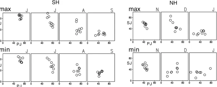
[26] Figure 11 displays the scatter diagram of the SJ and PJ as in Figure 6, but separated for solar maximum and minimum phases. The diagrams are plotted from June through September for the SH and from November through January for the NH, which correspond to climatological phase II and the beginning of phase III. July and December correspond to the period of the jet shift during solar maxima, as can be seen in Figure 9. Accordingly, the scatter diagram of July and December in the maximum phase in Figure 11 exhibits a clear seesaw between SJ and PJ with the bimodal feature of the distribution. A similar feature persists in SH until August, although it is less clear. The seesaw observed in July during solar minima no longer persists in August because SJ is weaker during solar minima. A similar weak seesaw is observed in November in the NH during the minimum phase, but it disappears in December. These differences correspond well to the slower speed of the seasonal evolution during the solar maximum phase, as depicted in Figure 9. Thus the influence of the solar cycle can still be detected as a modulation of the seasonal march despite the large year-to-year variation.
[27] Finally, meridional sections are shown to investigate the global aspect of the solar response. Figure 12 displays the composite difference between the solar maximum and minimum phases in zonal mean zonal winds (contours) and
E-P flux (arrows), while Figure 13 shows the difference in zonal mean temperatures (contours) and residual velocity (arrows). Figures are plotted so that the equator and winter pole are located on the left and right side, respectively, to facilitate a comparison between the SH (left-hand) and NH (right-hand). All variables are weighted by the cosine of latitude to reduce the large variability in high latitudes. The E-P fluxes are scaled by the inverse of the pressure to highlight variations in the upper levels. The divergence of the E-P flux is not explicitly shown in the present analysis. However, equation (1) is approximated as
divF¼ ðr0acosfÞfv*: ð3Þ
Thus it can easily be inferred from the meridional velocity of the residual circulation.
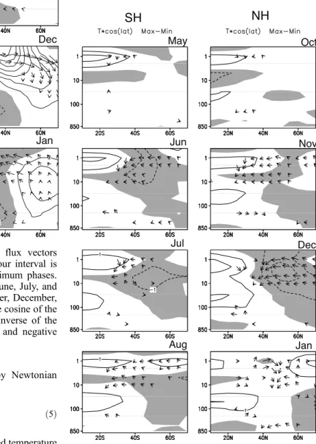
[28] In zonal wind field (Figure 12), no important solar signal is found in May in the SH. Stronger westerly anomalies develop in the subtropics during June and July. The planetary waves are deflected by these wind anomalies and propagate less equatorward. A divergence of the E-P flux consequently occurs in the midlatitudes, which induces less poleward residual circulation and less upwelling in the subtropics of the upper stratosphere (Figure 13). Although zonal wind anomalies shift slightly poleward in August, a similar smaller upwelling situation persists in the sub-tropics. High-temperature anomalies develop in the equato-Figure 9. The same phase diagram as in Figure 4, but for the means of different solar cycle phases. (a)
SH solar maximum, (b) SH solar minimum, (c) NH solar maximum, (d) NH solar minimum. Closed and open circles indicate the starting periods of phases II and III, respectively. The numbers indicate the time with the pentad counted from the winter solstice. Winter solstices are represented by crosses. Thick solid lines indicate periods corresponding to the month of July in the SH and December in the NH.
Figure 10. The same as in the top panels of Figure 5, but for solar maximum (top panels) and minimum (bottom panels) phases. Left and right panels are for the SH and NH.
rial lower stratosphere from June to August in association with the reduced upwelling.
[29] In the NH winter, no solar related zonal wind anomalies are found in October. Positive zonal wind anomalies develop in the subtropics during November and December. The planetary waves are deflected poleward, similar to the SH from June through August. Accordingly, poleward meridional circulation is reduced in the midlati-tudes and upwelling is suppressed in the subtropics. The positive zonal wind anomalies shift to the polar region in January, and negative anomalies appear in the subtropics associated with an enhanced equatorward propagation of waves. Convergence of the E-P flux around 40N latitude produces anomalous downwelling around 50N and upwell-ing around 30N. A decrease of temperature is observed in the lower latitudes, in contrast to increased temperatures in the polar region. Development of higher-temperature regions in the equatorial lower stratosphere during Novem-ber and DecemNovem-ber coincide with the reduced poleward residual circulation in the upper stratosphere, similar to the SH.
4. Discussion 4.1. Seasonal March
[30] The seasonal evolution of the stratopause jet during winter can be characterized by three stages in both hemi-spheres. The SJ velocity increases monotonically with the advancement of the season during the first phase. This variation is regular for each year, so this phase can be considered to be a radiatively controlled state. The PJ becomes weaker and the polar stratosphere warms up during the third phase. This stage may be considered to be a dynamically controlled state. Then, the second phase can be transitional stage from a radiatively controlled state to one dynamically controlled. During this stage poleward shift of the westerly jet is observed [Shiotani et al., 1993; Kuroda and Yamazaki, 1996; Dunkerton, 2000]. It is interesting to note that the bimodal feature appears in the
SJ during this phase (Figure 5). We have shown that the SJ continues to increase and that the beginning of the jet shift is delayed during solar maxima (Figure 9). This can be easily understood because increased solar radiative forcing during the maximum phase maintains the stratopause cir-culation longer in a radiatively controlled state, and the transition to a dynamically controlled state occurs later.
[31] The results of the analysis indicate that the velocity of SJ changes more than 10 ms1 between the solar maximum and minimum phases (see Figures 9 and 12). This significant response cannot be obtained without changes in the wave mean flow interaction, as suggested in Figure 7. We will discuss below using a conceptual model how weak solar radiation changes can produce substantial effects.
4.2. Conceptual Model
[32] Fels[1987] discussed dynamical response to changes in radiative forcing in the winter stratosphere. We use the same conceptual model here to discuss the solar cycle response. We consider a zonally averaged Boussinesq f-plane quasi-geostrophic model for the residual circulation for simplification. (For the complete set of the transformed Eulerian-mean equations, seeAndrews et al.[1987]).
Utfv*¼divF
TtþN2w*¼ ðR=HÞQ
fUz¼ðR=HÞTy
vy*þwz*¼0; ð4Þ
where U and T are the zonal mean zonal wind and temperature;v* and w* are the zonal mean northward and upward components of the residual circulation; f, Coriolis parameter; N, buoyancy frequency; R, universal gas constant; and H, scale height. F is the E-P flux, and the suffixes denote the derivatives.
Figure 11. Same as Figure 6, but for solar maximum (top panels) and minimum (bottom panels) phases. The diagrams are plotted from June through September for the SH (four left side panels) and from November through January for the NH (three right side panels).
[33] Radiative forcing is approximated by Newtonian heating as
Q¼ðTradTÞ=t; ð5Þ
WhereTradandtare the radiatively determined temperature
and relaxation time. Thus the following relation for the steady state is obtained from the above equations.
ðf=NÞ2½ðUUradÞ=tzz¼ðdivFÞyy ð6Þ
Where Urad is the radiatively determined zonal wind
velocity, f (Urad)z = (R/H) (Trad)y. If the horizontal and
vertical scales of the forcing are L and D, (6) can be approximated as
UradU
ð Þ=tðD=LÞ2ðN=fÞ2divF Fx ð7Þ
[34] It can be seen that the zonal wind velocity U becomes radiatively determined if the wave forcing Fx is
absent. It should also be noted that the wave forcing depends strongly on the zonal wind velocity, Fx (U).
Equation (7) can be graphically solved as an intersection of two curves, (UradU)/tandFx(U), once the form ofFx
(U) is specified. There is a certain range of velocity at which the waves can propagate efficiently in the westerly jet [Charney and Draizin, 1961]. Planetary waves cannot
Figure 12. Composite differences of E-P flux vectors (arrows) and zonal mean zonal winds (contour interval is 2m/s) between the solar maximum and minimum phases. (left) SH winter: from top to bottom, May, June, July, and August. (right) NH winter: October, November, December, and January. All variables are weighted by the cosine of the latitude, and the E-P flux is scaled by the inverse of the pressure. Zero contour lines are suppressed and negative values are shaded.
Figure 13. The same as in Figure 12, except for the composite differences of the meridional circulation (arrows) and zonal mean temperatures (contour interval is 1 K). Figures 12 and 13 are displayed so as the lower latitude are on the left side irrespective of the hemisphere.
propagate into the upper stratosphere when the zonal wind speed is too strong or too weak and their impact becomes small.
[35] Figure 14a schematically displays the solution of equation (7) for three different situations during the course of a normal cold season. (i) In early winter when the wave forcing is small, zonal winds balance at large velocitiesUh
near the one radiatively determined. (ii) Two stable states are possible when the wave amplitudes increase, one for strong zonal winds Uhwith small wave forcingFxand the
other for weak zonal winds Ul and large wave forcingFx.
(iii) Only the dynamically controlled weak wind stateUlis
possible if the wave amplitude grows further or the radiative forcing decreases after the solstice.
[36] There is little change in the cases of (i) or (iii) if a small variation in wave forcing occurs, because the wind velocity remains near those radiatively determined or dynamically determined. However, the wind could be either very strong or very weak in the case of (ii), where two stable solutions are possible. The wave forcing may change from one year to the next, so the largest interannual variability is expected during the transition period (ii). This explains the characteristics of the seasonal evolution of SJ and its interannual variability, as shown in Figure 5a. The radia-tively controlled state lasts longer, until stage (ii), if the radiative forcing increases during solar maxima (Figure 14b), and the transition period then occurs in stage (iii). Thus a significant impact from the solar cycle can be observed around the transition period. While year-to-year variations in wave forcing are expected, long-term changes in solar radiative forcing create systematic deviations of the system towards a radiatively controlled state.
[37] This conceptual model explains well the character-istics of the climatological seasonal march of SJ as well as that related to the solar cycle. The large solar signal should be a consequence of the bimodal nature of the winter atmosphere due to the interaction with planetary waves [Holton and Mass, 1976; Yoden, 1987]. However, it must
be noted that substantial changes in SJ are primarily produced by the interaction with meridionally propagating waves (Figure 7), not with those vertically propagated. Also, the interannual variation of SJ may not necessarily be related to a change in the tropospheric wave sources, but can arise from changes in propagation conditions within the stratosphere. For example, some relationship with the phase of the equatorial QBO has been observed in the NH. 4.3. Lower Stratospheric Effects
[38] The influence of the solar cycle manifests in early winter as a persistent subtropical jet in the upper strato-sphere and lower mesostrato-sphere. The winter stratostrato-sphere becomes a dynamically controlled state in late winter because of increased wave activity and decreased radiative forcing. Positive anomalies created by solar influence in the subtropics propagate poleward and downward from Decem-ber to January (Figure 12). Negative anomalies appear in January in the subtropics and develop and shift poleward in February, while positive anomalies migrate further down-ward in the troposphere. This behavior is similar to the internal mode of variation in the polar night jet (PJO) during winter [Kuroda and Kodera, 2001]. Thus this process can be understood as a modulation of the PJO by solar-induced anomalies, which is discussed in more detail byKuroda and Kodera [2002]. This downward penetration of the solar
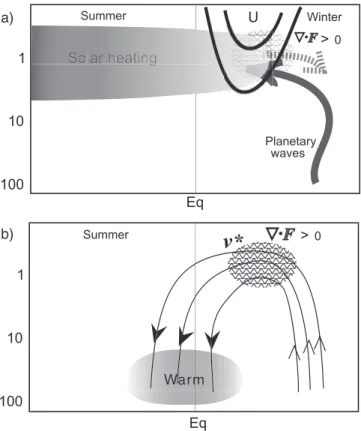
Figure 15. Schematic illustration of the solar influence on the lower stratosphere. (a) Stronger SJ due to increased solar forcing during the maximum phase deflects planetary waves from the subtropics (dashed arrow), which creates anom-alous divergence of the E-P flux (stippled). (b) Decrease in wave forcing results in reduces BD circulation (arrows) and warming in the tropical lower stratosphere (shading). For more detail, see section 4.2.
Figure 14. Schematic illustration of the conceptual model showing the dynamical impact of radiative forcing changes in the winter atmosphere for (a) normal conditions and (b) increased radiative forcing. (See section 4.3 for more detail.)
influence can be well reproduced by a general circulation model (GCM) simulation [Shindell et al., 1999].
[39] Another possible downward extension of the solar influence is through changes in meridional circulation. The upper stratospheric circulation tends to remain longer in a radiatively controlled state during the solar maximum and is characterized by a strong zonal mean flow and reduced wave forcings. The Brewer Dobson (BD) circulation is considered to be driven by extratropical wave forcing in the winter hemisphere [e.g.,Holton et al., 1995]. Thus the BD circu-lation should be weakened during the solar maximum.
[40] In fact, the results of the analysis indicate that a stronger subtropical jet is maintained longer in the winter during the solar maximum (Figures 12 and 13). The refractive index becomes small or negative at the poleward flank of the jet when its core is situated in the subtropics [Kodera et al., 1997]. This negative region of refractive index in the midlatitudes of the stratopause efficiently deflects planetary waves propagating from higher latitudes. The decrease of wave driving in the subtropics can be seen as reduced upwelling in the equatorial region (see July and December in Figures 12 and 13), which creates higher temperatures in the equatorial stratosphere. Changes in wave driving in the winter stratosphere can produce a global impact that extends from the winter to summer hemisphere by modulating the BD circulation [e.g., see Garcia, 1987; Randel, 1993]. In this way, the solar influence in the winter upper stratosphere and stratopause regions can be extended into the summer lower stratosphere [van Loon and Shea, 2000]. The above mentioned process is schematically illus-trated in Figure 15. Thus an increase in radiative heating in the stratopause region creates secondary warming in the lower stratosphere where the radiative relaxation time is long [Randel et al., 2002]. It must be noted, however, that the equatorial upwelling is critically dependent on the latitudinal structure of the wave driving [Plumb and Elusz-kiewic, 1999; Tung and Kinnersley, 2001]. Wave driving must extend sufficiently to the lower latitudes to produce vertical motion in the equatorial region; otherwise, meri-dional circulation closes within the midlatitudes of the winter hemisphere.
[41] The impact of meridional circulation in the equatorial stratosphere can be observed during the period when a stronger SJ remains in the subtropics (June, July, and August in the SH and November and December in the NH). Convergence of the E-P flux occurs in the polar region after the poleward shift (September in the SH and January in the NH), which creates poleward residual circulation; the downward flow produces polar warming, while the upward flow produces some cooling in the low latitudes. This explains well the seasonal structure of the solar signal in the equatorial lower stratosphere. The greatest solar response in the equatorial temperature at 70 hPa occurs at two periods, one around August and the other around December [Labitzke, 2001, Figure 7]. Although, there is a problem for the estimation of the solar cycle temperature variation due to changes in observing systems [see Hood, 2002], interseasonal temperature variations in Figure 13, should be less affected by such technical problems.
[42] In this study we focused on the dynamical response of the solar cycle. Changes in meridional circulation affect the distribution of long-lived chemical compounds by the
transport process. Ozone in the lower stratosphere in partic-ular, with a long lifetime and very steep vertical gradient, is very sensitive to changes in the vertical transport. It can be seen that the ozone concentration in the equatorial lower stratosphere changes together with the temperature in response to wave driving [Randel, 1993]. Recent observa-tional study [Hood, 2002] suggests a solar cycle ozone variation caused by a wave-driven meridional circulation. Also, simulations of solar cycle using 3-D chemical models produce increase in ozone concentration in the equatorial lower stratosphere during the solar maximum condition [Labitzke et al., 2002], whereas such response is absent in 2-D models [Brasseur, 1993;Haigh, 1994; Fleming et al., 1995]. These results are consistent with the present study. 5. Concluding Remarks
[43] The stratopause circulation evolves from a radia-tively controlled state to one dynamically controlled during winter. This transition period has been observed to be characterized by a poleward shift of the jet. The solar cycle effect appears as a change in the balance between the radiatively and dynamically controlled states; SJ remains in the radiatively controlled state longer and reaches higher speeds during solar maximum phases. The dynamical response to the solar cycle together with the nature of the interannual variability in SJ can be understood using a conceptual model by Fels [1987] that includes the inter-action with planetary waves.
[44] Changes in the wave mean flow interaction produced in the upper stratosphere and stratopause region can prop-agate into the lower stratosphere as modulation of the internal mode of variation in the winter stratosphere. But also, changes in the wave mean flow interaction produce changes in the BD circulation. The first process is signifi-cant in the middle and high latitudes, whereas the latter is prominent in the equatorial region.
[45] The role of the equatorial QBO is not discussed in the present paper, but it should be clarified in the future study. It is important to have a ‘‘testable mechanism’’ that can be verified through model simulations and experiments. Our analysis also indicates the importance of the seasonal march, in particular the evolution of the SJ. Existing general circulation models fail to reproduce a realistic seasonal march of the SJ [Pawson et al., 2000]. Further improvement of the climate of GCMs is required for a more realistic simulation of the solar response.
[46] Acknowledgments. The authors thank K. Matthes for useful comments and discussions. Solar radio flux data were obtained from the National Geophysical Data Center, NOAA (http://web.ngdc.noaa.gov/stp/ stp.html).
References
Andrews, D. G., J. R. Holton, and C. B. Leovy,Middle Atmosphere Dy-namics, 489 pp., Academic, San Diego, Calif., 1987.
Balachandran, N. K., and D. Rind, Modeling the effects of UV variability and the QBO on the troposphere/stratosphere system, I, The middle atmo-sphere,J. Clim.,8, 2058 – 2079, 1995.
Brasseur, G., The response of the middle atmosphere to long-term and short-term solar variability: A two-dimensional model, J. Geophys. Res.,98, 23,079 – 23,090, 1993.
Charney, J. G., and P. G. Draizin, Propagation of planetary-scale distur-bances from the lower into the upper atmosphere,J. Geophys. Res.,66, 83 – 109, 1961.
Christiansen, B., Downward propagation of zonal mean zonal wind anoma-lies from the stratosphere to the troposphere: Model and reanalysis,J. Geophys. Res.,106, 27,307 – 27,322, 2001.
Dunkerton, T. J., Midwinter deceleration of the subtropical mesospheric jet and interannual variability of the high-latitude flow in UKMO analysis,J. Atmos. Sci.,57, 3838 – 3855, 2000.
Fels, S. B., Response of the middle atmosphere to change O3and CO2—A speculative tutorial, inTransport Processes in the Middle Atmosphere, edited by G. Visconti and R. Garcia, pp. 371 – 386, D. Reidel, Norwell, Mass., 1987.
Fleming, E. L., S. Chandra, C. H. Jackman, D. B. Considine, and A. D. Douglass, The middle atmospheric response to short and long term solar UV variations: Analysis of observations and 2D model results,J. Atmos. Terr. Phys.,57, 333 – 365, 1995.
Garcia, R. R., On the meridional circulation of the middle atmosphere,J. Atmos. Sci,44, 3599 – 3609, 1987.
Geller, M. A., and J. C. Alpert, Planetary wave coupling between the tropo-sphere and the middle atmotropo-sphere as a possible Sun-weather mechanism, J. Atmos. Sci.,37, 1197 – 1215, 1980.
Haigh, J. D., The role of stratospheric ozone in modulating the solar radia-tive forcing of climate,Nature,370, 544 – 546, 1994.
Haigh, J. D., A GCM study of climate change in response to the 11-year solar cycle,Q. J. R. Meteorol. Soc.,125, 871 – 892, 1999.
Haynes, P. H., C. J. Marks, M. E. McIntyre, T. G. Shepherd, and K. P. Shine, On the ‘‘downward control’’ of extratropical diabatic circulation by eddy-induced mean zonal forces,J. Atmos., Sci.,48, 651 – 678, 1991. Hirota, I., T. Hirooka, and M. Shiotani, Upper stratospheric circulation in the two hemispheres observed by satellites,Q. J. R. Meteorol. Soc.,109, 443 – 454, 1983.
Holton, J. R., and C. Mass, Stratospheric vacillation cycles,J. Atmos. Sci., 33, 2218 – 2225, 1976.
Holton, J. R., P. H. Haynes, M. E. McIntyre, A. R. Douglass, R. B. Rood, and L. Pfister, Stratospheric-troposphere exchange,Rev. Geophys.,33, 403 – 439, 1995.
Hood, L. L., Effects of solar UV variability on the stratosphere, inSolar Variability and Its Effect on the Earth’s Atmospheric and Climate System, AGU Monogr. Ser., edited by J. Pap et al., AGU, Washington, D. C., in press, 2002.
Hood, L. L., J. L. Jirikowic, and J. P. McCormack, Quasi-decadal bility of the stratosphere: Influence of long-term solar ultra violet varia-tions,J. Atmos. Sci.,50, 3941 – 3958, 1993.
Kalnay, E., et al., The NCEP/NCAR 40-year reanalysis project,Bull. Am. Meteorol. Soc.,77, 437 – 471, 1996.
Kodera, K., On the origin and nature of the interannual variability of the winter stratospheric circulation in the Northern Hemisphere,J. Geophys. Res.,100, 14,077 – 14,087, 1995.
Kodera, K., and K. Yamazaki, Long-term variation of upper stratospheric circulation in the Northern Hemisphere in December,J. Meteorol. Soc. Jpn.,68, 101 – 105, 1990.
Kodera, K., K. Yamazaki, M. Chiba, and K. Shibata, Downward propaga-tion of upper stratospheric mean zonal wind perturbapropaga-tion to the tropo-sphere,Geophys. Res. Lett.,17, 1263 – 1266, 1990.
Kodera, K., J. McCormack, and M. Giorgetta, Influence of the solar cycle on climate through stratospheric processes, inThe Stratosphere and Its Role in the Climate System, edited by G. Brasseur, pp. 83 – 98, Springer-Verlag, New York, 1997.
Kuroda, Y., and K. Kodera, Variability of the polar-night jet in the Northern and Southern Hemispheres,J. Geophys. Res.,106, 20,703 – 20,713, 2001. Kuroda, Y., and K. Kodera, Effect of the solar cycle on the polar-night jet
oscillation,J. Meteorol. Soc. Jpn.,80, 973 – 984, 2002.
Kuroda, Y., and K. Yamazaki, Poleward jet-shift in the Southern Hemi-sphere winter simulated with a general circulation model,Pap. Meteorol. Geophys.,47, 47 – 56, 1996.
Labitzke, K., Sunspots, the QBO, and the stratospheric temperature in the north polar region,Geophys. Res. Lett.,14, 535 – 537, 1987.
Labitzke, K., The global signal of the 11-year sunspot cycle in the strato-sphere: Differences between solar maxima and minima,Meteorol. Z.,10, 83 – 90, 2001.
Labitzke, K., and H. van Loon, Association between the 11-year solar cycle, the QBO and the atmosphere, I, The troposphere and stratosphere
in the Northern Hemisphere in winter,J. Atmos. Terr. Phys.,50, 197 – 206, 1988.
Labitzke, K., J. Austin, N. Butchart, J. Knight, M. Takahashi, M. Nakamo-to, T. Nagashima, J. Haigh, and V. Williams, The global signal of the 11-year solar cycle in the stratosphere: Observations and model results,J. Atmos. Sol. Terr. Phys.,64, 203 – 210, 2002.
Lean, L., J. Rottman, G. J. Kyle, H. L. Woods, T. N. Hickey, and J. R. Pugga, Detection and parameterization of variations in solar mid and-near-ultraviolet radiation (200 – 400 nm),J. Geophys. Res.,102, 29,939 – 29,956, 1997.
McCormack, J. P., and L. L. Hood, Apparent solar cycle variation of upper stratospheric ozone and temperature: Latitude and seasonal dependences, J. Geophys. Res.,101, 20,933 – 20,944, 1996.
Pawson, S., et al., The GCM-reality intercomparison project for SPARC (GRIPS): Scientific issues and initial results,Bull. Am. Meteorol. Soc., 81, 781 – 796, 2000.
Pittock, B. A., A critical look at long-term Sun-weather relationships,Rev. Geophys. Space Phys.,16, 400 – 420, 1978.
Plumb, R. A., On the seasonal cycle of stratospheric planetary waves,Pure Appl. Geophys.,130, 223 – 242, 1989.
Plumb, A., and J. Eluszkiewic, The Brewer-Dobson circulation: Dynamics of the tropical upwelling,J. Atmos. Sci.,56, 868 – 890, 1999.
Randel, W. J., Global atmospheric circulation statistics, 1000-1 mb,NCAR Tech. Note NCAR/TN-366 + STR, 256 pp., Nat. Cent. for Atmos. Res., Boulder, Colo., 1992.
Randel, W. J., Global variation of zonal mean ozone during stratospheric warming events,J. Atmos. Sci.,50, 3308 – 3321, 1993.
Randel, W., R. R. Garcia, and F. Wu, Time-dependent upwelling in the tropical lower stratosphere estimated from the zonal-mean momentum budget,J. Atmos. Sci.,59, 2141 – 2152, 2002.
Rind, D., and N. K. Balachandran, Modeling the effects of UV variability and the QBO on the troposphere/stratosphere system, II, The troposphere, J. Clim.,8, 2080 – 2095, 1995.
Shindell, D., N. K. Rind, N. K. Balachandran, J. Lean, and P. Lonergan, Solar cycle variability, ozone, and climate,Science,284, 305 – 308, 1999. Shindell, D., G. A. Schmidt, R. L. Miller, and D. Rind, Northern Hemi-sphere winter climate response to greenhouse gas, ozone, solar, and volcanic forcing,J. Geophys. Res.,106, 7193 – 7210, 2001.
Shiotani, M., N. Shimoda, and I. Hirota, Interannual variability of the stratospheric circulation in the Southern Hemisphere,Q. J. R. Meteorol. Soc.,199, 531 – 546, 1993.
Soel, D.-I., and K. Yamazaki, Residual mean circulation in the stratosphere and upper troposphere: Climatological aspects,J. Meteorol. Soc. Jpn.,77, 985 – 996, 1999.
Solomon, S., R. W. Portmann, R. R. Garcia, L. W. Thomason, L. R. Poole, and M. P. McCormic, The role of aerosol trends and variability in anthro-pogenic ozone depletion at northern midlatitudes,J. Geophys. Res.,101, 6713 – 6727, 1996.
Stratospheric Processes and Their Role in Climate (SPARC), Assessment of trends in vertical distribution of ozone,Rep. 43, edited by N. Harris, R. Hudson, and C. Phillips, World Meteorol. Org. Ozone Res. and Monit. Proj., Geneva, 1998.
Tung, K. K., and J. S. Kinnersley, Mechanisms by which extratropical wave forcing in the winter stratosphere induces upwelling in the summer hemi-sphere,J. Geophys. Res.,106, 22,781 – 22,791, 2001.
van Loon, H., and K. Labitzke, The influence of the 11-year solar cycle on the stratosphere below 30km: A review, Int. Space Sci. Inst., Bern, Swit-zerland, 2000.
van Loon, H., and D. J. Shea, The global 11-year solar signal in July – August,Geophys. Res. Lett.,27, 2965 – 2968, 2000.
Yoden, S., Bifurcation properties of a stratospheric vacillation model,J. Atmos. Sci.,44, 1723 – 1733, 1987.
Yoden, S., An illustrative model of seasonal and interannual variations of the stratospheric circulation,J. Atmos. Sci.,47, 1845 – 1853, 1990.
K. Kodera and Y. Kuroda, Meteorological Research Institute, 1-1 Nagamine, Tsukuba, Ibaraki 305-0052, Japan. ([email protected]; [email protected])