Real exchange rate volatility, financial crises and exchange-rate regimes

(1)

Real exchange rate volatility, financial crises and

exchange-rate regimes

Amalia Morales-Zumaquero

(Departamento of Economic Theory and History, Universidad de Málaga, Campus El Ejido, 29071 Málaga, Spain)

[email protected]

Corresponding author: Simón Sosvilla-Rivero

(Department of Quantitative Economics, Universidad Complutense de Madrid. Campus de Somosaguas, 28223 Madrid, Spain)

[email protected]

Published in Applied Economics, Vol. 46, 2014, 826-847 Abstract

This paper examines real exchange rate (RER) volatility in eighty countries around the world, during the period 1970 to 2011. Two main questions are raised: are structural breaks in RER volatility related to changes in exchange-rate regimes or financial crises? And do these two events affect the permanent and transitory components of RER volatility? To answer them, we employ two complementary procedures that consist in detecting structural breaks in the RER series and decomposing volatility into its permanent and transitory components. Our results suggest that structural breaks in RER volatility coincidence with financial crises and certain changes in nominal exchange-rate regimes. Moreover, our findings confirm that RER volatility does increase with the global financial crises and detect that the more flexible the exchange rate regime, the higher the volatility of the RER using a de facto exchange rate classification.

Keywords: Financial Crisis, Structural Breaks, Component-GARCH Model, Real Exchange Rates

(2)

1. Introduction

An important challenge to exchange rate theory is the solution to the puzzle that real exchange rates (RERs) are more volatile than what most models can account for. Moreover, there is a great disagreement in the finance literature about the behaviour of nominal exchange rate volatility under alternative exchange rate arrangements. Flood and Rose (1995) highlight empirically a positive link between exchange rate volatility and flexible exchange rate regimes while Valachy and Kocenda (2003) find either positive or negative link according to the countries under investigation. Friedman (1953) argues that exchange rate volatility cannot be reduced by switching from floating to fixed exchange rates. Lastly, there is a strand of theoretical literature that supports that financial integration may reduce exchange rate volatility (see, for example, Obstfeld, 1984), although the empirical studies on the effects of globalization on exchange rate volatility remain non-conclusive: while Krugman and Obstfeld (2003) showed that globalization lead to exchange rate fluctuations, Hau (2002) and Calderón (2004) find a positive effect of liberalization on the reduction of the RER volatility. Moreover, Dornbusch et al. (1995) and De Gregorio et al. (2000) suggest that regardless of exchange regimes; financial integration can make countries vulnerable to the external shocks, while Coudert et al. (2011) show that, for most countries in their sample, exchange rate volatility increases more than proportionally with the global financial crises. This is especially relevant since, from a historical perspective, financial crises seem to be more like the rule rather than the exception (see Bordo et al., 2001 and Reinhart et al., 2010; among others).

Since RER volatility has important implications for consumption, investment, economic growth, and trade flows (see Dellas and Zilberfarb, 1993; Campa and Goldberg, 1995; Darby et al., 1999; Frankel and Rose 2002; Broda and Romalis 2013; and Viera et al., 2013, among others), establishing the relative importance of financial crises and exchange-rate regimes on RER volatility is a crucial question.

The majority of the existing literature investigates the effects of exchange rate volatility on a number of macroeconomic variables, e.g. growth (Bagella et al., 2006) or trade (Baum and Caglayan, 2010). However, there is a lack of sufficient studies examining if

(3)

changes in volatility are driven by changes in nominal exchange-rate regimes or financial crises.

Regarding previous evidence on this issue we can refer, among others, to Kocenda (2005) (who endogenously searches for the single most decisive structural break in exchange rate for a group of European transition countries, detecting breaks that are frequently associated with major changes in exchange rate regime), Balg and Mecalf (2010) (who investigate the impact of the volatility of the underlying macroeconomic fundamentals on exchange rate volatility, concluding that in the long run the volatility of the money supply is the sole determinant, whereas in the short run overshooting is found), Morales-Zumaquero and Sosvilla-Rivero (2010) (who examine the real exchange rate behaviour for a set of 22 OECD and 20 non-OECD countries during the 1960–2006 period, obtaining that there is clear evidence in favour of the non-neutrality of nominal exchange rate regime regarding real exchange rate volatility for developed countries, but not in the case of developing or emerging countries), Carrera and Vuletin (2013) (who examine a dataset for 63 countries over the period 1946–2007 finding that alternative exchange rate regimes affect short-term real exchange rate volatility differently), and Caporale et. al (2013) (who find that external, real and monetary shocks can account for the volatility of real exchange rates in emerging economies, with international financial integration being a major driving force).

This paper attempts to contribute to the empirical literature in this area raising two main questions: are structural breaks in RER volatility related to changes in exchange-rate regimes or financial crises? And do these two events affect the permanent and transitory components of RER volatility? To that end, we use a comprehensive data set including developed and developing countries for the 1970-2011 period, to examine whether the choice of exchange rate regime and the occurrence of a financial crisis are associated with structural breaks in RER volatility and whether they affect its permanent and transitory components.

In relation to the relevance of nominal exchange rate regimes and financial crises in explaining structural breaks in RER volatility, we use two econometric methods for testing for structural breaks: the OLS-based tests to endogenously detect multiple structural breaks, as proposed by Bai and Perron (1998, 2003), and several procedures

(4)

based on Information Criterion together with the so-called sequential procedure suggested by Bai and Perron (2003). Once these structural breaks in RER volatility are detected, we examine if they are associated with major banking, currency and debt crises and whether they coincide with changes in nominal exchange rate regimes.

As for the evaluation of effects of nominal exchange rate regimes and financial crises on RER volatility, we use the component GARCH model proposed by Engle and Lee (1999) to decompose RER volatility into a permanent long-run trend component and a transitory short-run component that is mean-reverting towards the long-run trend.

Our results suggest that structural breaks in RER volatility coincide with financial crises and certain changes in nominal exchange-rate regimes. Moreover, our findings confirm that exchange rate volatility does increase with the global financial crises and suggest that the more flexible the exchange rate regime, the higher the volatility of the RER using a de facto exchange rate classification to capture the policies implemented by countries regardless of the regime reported by the country’s authorities.

The rest of this paper is structured as follows. Section 2 describes the econometric methodology adopted in this study. Section 3 presents the data and the empirical result, and Section 4 offers some concluding remarks.

2. Econometric Methodology 2.1. Structural Breaks

Bai and Perron (1998, 2003) consider the following multiple linear regression with m breaks (m+1 regimes): . T ,..., T t , u δ z β x y , T ,..., T t , u δ z β x y , T ,..., t , u δ z β x y m t m ' t ' t t t ' t ' t t t ' t ' t t 1 (1) 1 1 1 2 1 2 1 1 + = + + = + = + + = = + + = + 

(5)

In this model, yt is the observed dependent variable at time t; xt (p×1)and zt )

1

(q× are vectors of covariates and β and δ_j (j=1,...,m+1)are the vectors of coefficients, respectively. Finally, u_t is the disturbance at time t. The break points

) ,...,

(T₁ T_m are unknown. The purpose is to estimate the unknown regression coefficients and the break points using a sample of T observations.

We consider a pure structural change model(p=0), where all the coefficients are subject to change, from the model in equation (1). In this sense, we specify each series as an AR(1) process and then, to detect multiple structural breaks in variance, we use the absolute value of the fitted residuals of the AR(1) models1. For this analysis we specify zt =

{}

1 .

To detect multiple structural breaks, we use the set of tests developed by Bai and Perron (1998, 2003): the sup F type test, the double maximum tests UDmax and WDmax and the test for  versus +1 breaks, labelled sup F_T

(

+1

)

test2. To run these tests it is necessary to decide the minimum distance between two consecutive breaks, h, that it, is obtain as the integer part of a trimming parameter, ε, multiplied by the number of observations T (we use ε =0.15 and allow up to four breaks).

To select the dimension of the models, we follow the method suggested by Bai and Perron (1998) based on the sequential application of the sup F_T

(

+1

)

test, the sequential procedure.

1_{Similarly, Stock and Watson (2002) use the absolute value of the fitted residuals of a VAR model to}

analyse changes in variance. Alternatively, Valentinyi-Endrész (2004) use the squared errors from a AR(1)-GARCH(1,1) model to compute changes in variance.

2

(6)

2.2. Permanent and Transitory Components

Engle and Lee (1999) proposed a “component-GARCH” (C-GARCH) model to decompose time-varying volatility into a permanent (long-run) and a transitory (short-run) component.

Consider the original GARCH model:

) ( ) ( 21 2 1 2 ω α ε ω β σ ω σt = + t₋ − + t₋ −

(2)

As can be seen, the conditional variance of the returns here has mean reversion to some time-invariable value, ω. The influence of a past shock eventually decays to zero as the volatility converges to this value ω_{according to the powers of (}α+β). The standard GARCH model therefore makes no distinction between the long-run and short-run decay behavior of volatility persistence.

For the permanent specification, the C-GARCH model replaces the time- invariable mean reversion value,ω, of the original GARCH formulation in equation (2) with a time variable component qt:

) ( ) ˆ ( ˆ 2 1 2 1 1 − − − − + − + = t t t t q q ω ρ ω ϕ ε σ

(3)

where, qt is the long-run time-variable volatility level, which converges to the long-run

time-invariable volatility level ωˆ according to the magnitude of ρ. This permanent component thus describes the run persistence behaviour of the variance. The long-run time-invariable volatility level ωˆ can be viewed as the long-run level of returns variance for the relevant sector when past errors no longer influence future variance in

(7)

any way. Stated differently, the value ωˆ can be seen as a measure of the ‘underlying’ level of variance for the respective series. The closer the estimated value of the ρ in equation (7) is to one the slower qt approaches ωˆ , and the closer it is to zero the faster it

approachesωˆ . The value ρ therefore provides a measure of the long-run persistence. The second part of C-GARCH model is the specification for the short-run dynamics, the behaviour of the volatility persistence around this long-run time-variable mean, qt:

) ( ) ( 1 2 1 1 2 1 2 − − − − − + − = − t t t t t t q γ ε q λ σ q σ (4)

According to this transitory specification, the deviation of the current condition variance from the long-run variance mean at time t (σ_t2−q_t) is affected by the deviation of the previous error from the long-run mean (ε_t2₋₁−q_t₋₁) and the previous deviation of the condition variance from the long-run mean( 1)

2

1 −

− − t

t q

σ . Therefore, in keeping with its GARCH theoretical background, the C-GARCH specification continues to take account of the persistence of volatility clustering by having the conditional variance as a function of past errors. As the transitory component describes the relationship between the short-run and long-run influence, decline rates of past shocks values of (γ+λ) closer to one imply slower convergence of the short-run and long-run influence decline rates, and values closer to zero the opposite. The value (γ+λ) is therefore a measure of how long this short-run influence decline rate is.

(8)

3. Data and Empirical Results 3.1. Data

We use monthly data of eighty bilateral real exchange rates against United States dollar, from January 1970 to December 20113, taken from the International Monetary Fund's International Financial Statistics and the Federal Reserve Board’s Financial Statistics.4 We consider six sets of countries: American countries (Canada, Mexico, Costa Rica, El Salvador, Guatemala, Honduras, Nicaragua, Panama, Dominican Republic, Jamaica, Trinidad and Tobago, Argentina, Brazil, Chile, Colombia, Ecuador, Paraguay, Peru, Uruguay and Venezuela); European countries (European Union-125, Austria, Belgium, Denmark, Finland, France, Germany, Greece, Italy, Ireland, Netherlands, Portugal, Spain, Sweden, United Kingdom, Czech Republic, Hungary, Poland, Norway, Russia, Switzerland and Turkey); Middle East countries (Israel, Jordan, Kuwait, Syria, Saudi Arabia); Oceania countries (Australia and New Zealand); Asian countries (Bangladesh, India, Indonesia, Malaysia, Pakistan, Philippines, Singapore, Sri Lanka, Thailand, China, Hong Kong, Japan, Korea and Taiwan) and African countries (Algeria, Egypt, Morocco, Tunisia, Benin, Cameroon, Congo, Cote d’Ivoire, Ghana, Kenya, Mozambique, Nigeria, Senegal, Sierra Leone, South Africa, Tanzania and Zambia).

All real exchange rate series have been corrected of outliers following the methodology developed by Gómez and Maravall (1996).6

3_{The sample size for Nicaragua covers the period 1988:1-2011:12.}

4_{Data collected by Mathew Shane, Economic Research Service, United States Department of}

Agriculture.

5

The European Union (EU) was established on 1 November 1993 with 12 Member States (Belgium, Denmark, France, Germany, Greece, Ireland, Italy, Luxembourg, Netherlands, Portugal, Spain and United Kingdom). Their number has grown to the present 28 through a series of enlargements In our analysis we use the original EU-12 as an additional “country”.

6

(9)

Given that the countries in our sample present different exchange rate regimes that can change under the period studied, we have used the “natural fine classification” of Reinhart and Rogoff (2004), updated to December 2010 by Ilzetzki, Reinhart and Rogoff (2011), to distinguish between a wide range of de facto regimes: 1) no separate legal tender; 2) pre announced peg or currency board arrangement; 3) pre announced horizontal band that is narrower than or equal to ±2%; 4) de facto peg; 5) pre announced crawling peg; 6) pre announced crawling band that is narrower than or equal to ±2%; 7) de factor crawling peg; 8) de facto crawling band that is narrower than or equal to ±2%; 9) pre announced crawling band that is wider than or equal to ±2%; 10) de facto crawling band that is narrower than or equal to ±5%; 11) moving band that is narrower than or equal to ±2% (i.e., allows for both appreciation and depreciation over time); 12) managed floating; 13) freely floating; 14) freely falling; 15) dual market in which parallel market data is missing.

As the tables in Ilzetzki, Reinhart and Rogoff (2011) provide monthly data until December 2010, we can identify the exact date of the change of regime. For 2011, we assume that there is not modification in the exchange rate regime.

Regarding the financial crisis dates, we make use of the information provided by Laeven and Valencia (2008) and Reinhart (2010). The former covers all systemically important banking, currency and debt crises (hereafter SBC, CC and DC, respectively) for the period 1970 to 2007 for 261 countries, while the later offers the individual timeline of public and private debts, banking, sovereign domestic and external debt crises , and hyperinflation, for 70 countries, from their independence to 2010.

(10)

3.2. Empirical Results

3.2.1. Structural Breaks Results

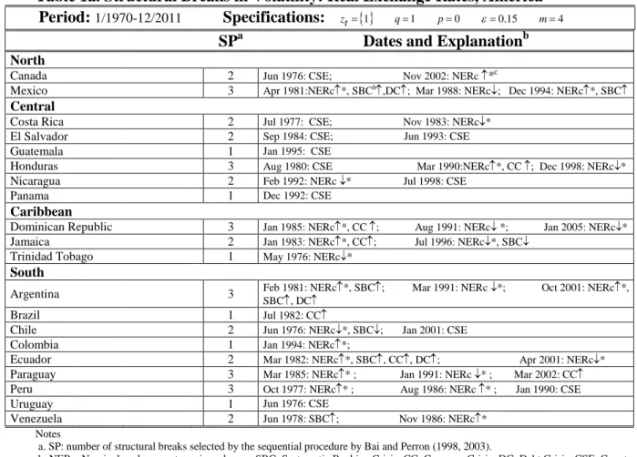
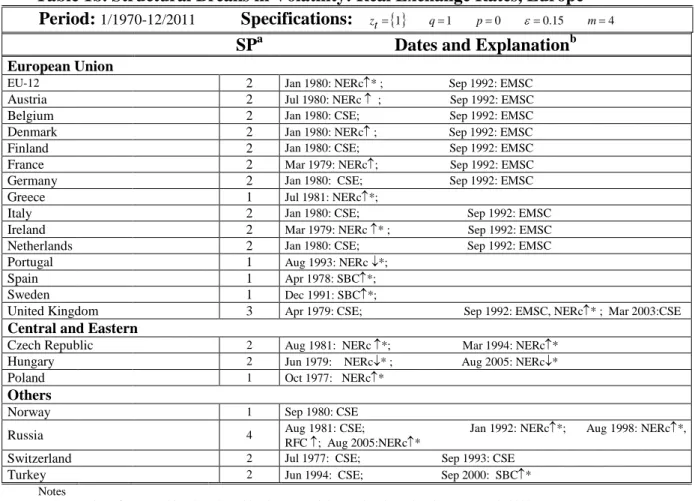
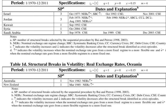
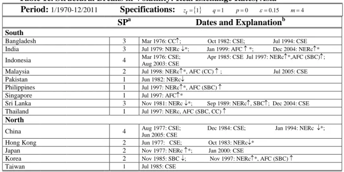
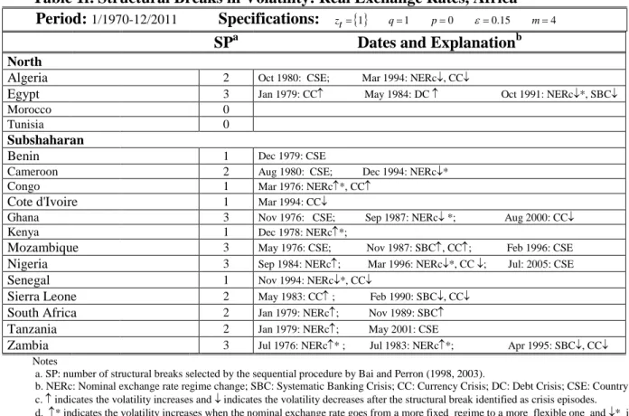
Tables 1a-f present the detected numbers and dates of structural breaks7 and their connection with an economic event for our examined set of countries. Recall that these breaks are searched endogenously from the data and our procedure does not rely on pre-test information to determine them, thereby avoiding the possible problem of “data mining”.

To facilitate the interpretation of Tables 1a-f, we have indicated with an arrow if volatility increases (↑) or decreases (↓) after the structural break identified as crisis

episodes (i.e., systematic banking crisis, SBC; currency crisis, CC and debt crisis, DC). As for the breakpoints associated with variations in the exchange rate regime (nominal exchange regime change, NERc), we have used the same convention, so an arrow pointing downwards (↓) would indicate the volatility decreases and an arrow pointing upwards (↑) would indicate the volatility decreases. Additionally, ↑* indicates the volatility increases when the nominal exchange rate goes from a more fixed regime to a more flexible one and ↓* indicates the volatility decreases when the nominal exchange rate goes from a more flexible regime to a more fixed one. Moreover, in Tables 1a-f, there is a set of breaks that can be associated with specific economic events of each examined country (that we have denoted as country specific events, CSE).

[Tables 1a-f, here]

7_{In order to save space, the numerical results of Bai and Perron’s tests are not reported in Table 1 but}

(11)

All in all, findings from our structural breaks analysis suggest several empirical regularities8. First, our results seem to indicate that exchange rate regimes do really matter, as we obtain evidence in favour of nominal regimes affecting RER variation. Second, we detect, in almost all cases that the more flexible the exchange rate regime, the higher the volatility of the RER, as well as an increase in RER volatility after a financial crisis in almost all cases. Third, we document an alteration in the nominal exchange rate regime towards a more flexible one after the event of a crisis.9 This result is in line with that of Fornaro (2011)’s, who claims the superiority of flexible exchange rate regimes compared to pegs both for the purpose of crisis times stabilization and as crises prevention devices. Finally, while two of the strongest financial crises, the Russian and Asian financial crises, have been detected using the procedure by Bai and Perron (1998, 2003), there is no evidence of a significant change in RER volatility around 2007 or 2008 capturing the recent global financial crisis. This could be related to the fact that various countries made have interfered in foreign exchange markets (using intervention and capital controls) to restrain tensions in the foreign exchange markets (see, e. g., Deutsche Bundesbank, 2010). Nevertheless, it is worth noting that institutional idiosyncrasies or major economic events are still at play, given the heterogeneity of break points detected across countries associated with country specific events. The reason for this heterogeneity is reserved for future research.

8

We summarize the results by pointing out the main regularities. The reader is asked to browse through Tables 1a to f to find evidence for particular countries or group of countries of her/his special interest and the respective estimated break points. A more detailed account of the results by groups of countries can be found in Morales-Zumaquero and Sosvilla-Rivero (2012).

9

(12)

3.2.2. Permanent and Transitory Components Results

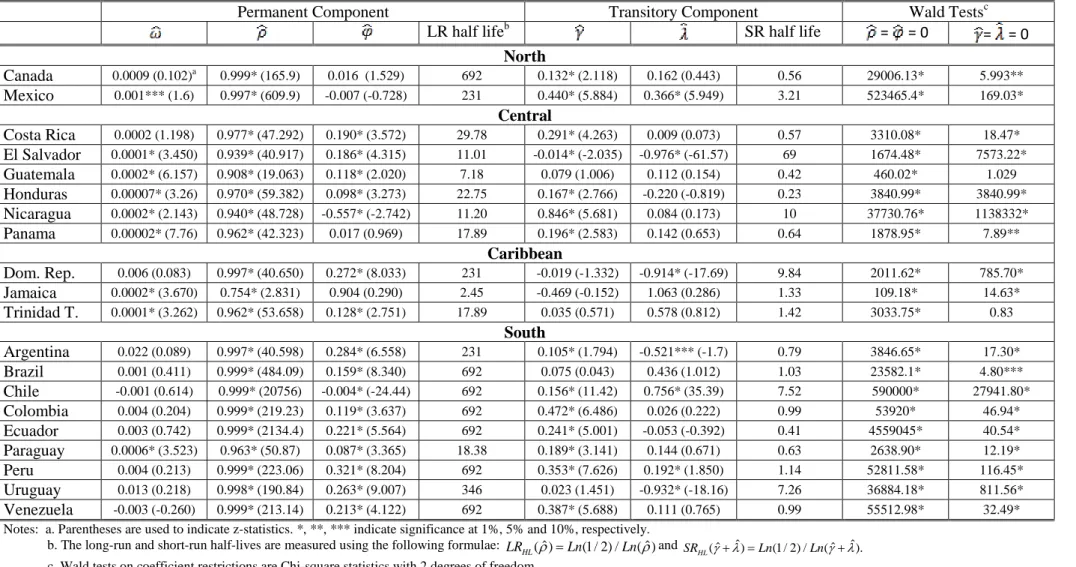
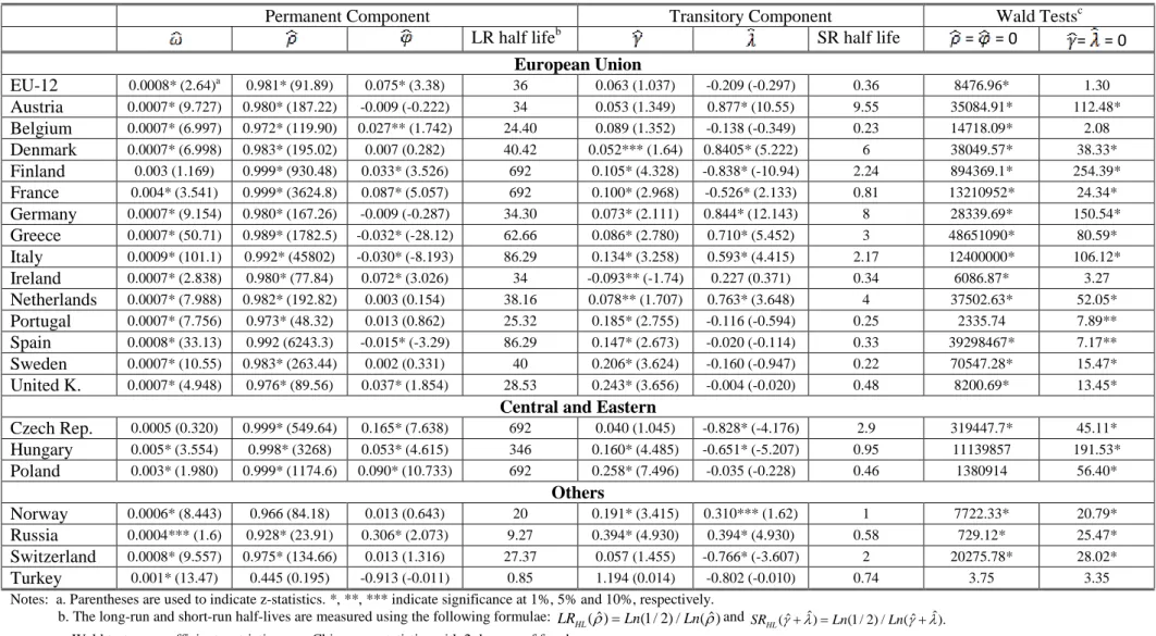
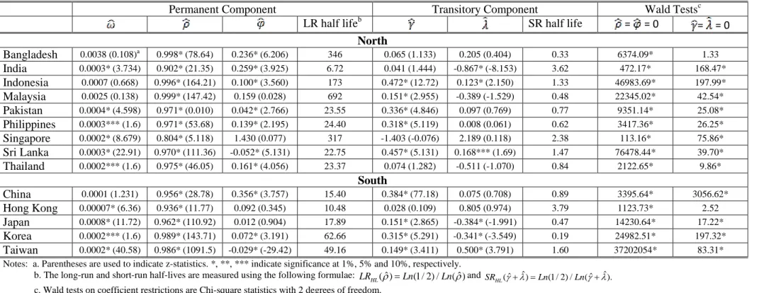
Tables 2a-f report coefficient estimates for the C-GARCH models obtained by maximum likelihood for each real exchange rate. Table 3 exhibits a summary of results with the numbers and percentages of significant coefficient estimates.

From these tables empirical results suggest a central message: evidence in favour that there exists a permanent-transitory component decomposition for our set of real exchange rates10. In addition, in order to evaluate the empirical relevance of our analysis, we compare the performance of the C-GARCH model to the GARCH model. It is worth noting that the C-GARCH model reduces to the GARCH (1, 1) model either = =0 or = = 0. On the basis of Wald tests on these coefficients, we can see the null hypothesis is decisively rejected in almost all cases in favour of C-GARCH specification over the GARCH(1,1) specification, giving further support for our specification strategy.

[Table 2a-f, here] [Table 3, here]

From visual inspection of figures plotting the estimated of the total conditional variance and its two components (permanent and transitory), of the monthly difference in real exchange rate for all countries under study, two regularities seem to appear11: (1) there is a change in volatility when a financial crisis occurs: sometimes the permanent

10_{This is the main regularity. The reader is asked to browse through Tables 2a to f and Table 3 to find}

evidence for particular countries or group of countries of her/his special interest. A more detailed account of the results by groups of countries can be found in Morales-Zumaquero and Sosvilla-Rivero (2012).

11_{To save space, we do not show here these figures. They are available in Morales-Zumaquero and}

(13)

component has smooth movements around the total GARCH volatility while the transitory component raises and other times the three volatilities (the total GARCH permanent and transitory) move together during a financial crisis; and (2) it looks that the transitory component is much more volatile, responding largely to economic events. Taken together, these findings imply that during financial crises, exchange rates are determined not only by traditional factors but also, to a major extent, by subjective perception of market participants.

Finally, and in line with Sarno and Valente (2006), a pattern seems to emerge relating countries with long periods of fixed exchange rate regimes and higher degree of persistence in RER volatility.

[Figures 1 to 6, here]

We further analyse the connection between the behaviour of the permanent-transitory components with both theoccurrence of a change in the nominal exchange rate regime and the existence of a SBC and/or a CC and/or a DC. Tables 4a-e and 5a-e show the results. In the first column of Tables 4a-e we present the dating of financial crises using the information provided by Laeven and Valencia (2008) and Reinhart (2010). In the first column of Tables 5a-e we present the structural breaks associated with a change in the nominal exchange rate regime. In the second column of Tables 4 and 5, we present the results of three variance equality tests (VET): the Bartlett test, the Levene test and the Brown-Forsythe test.12

12_{For details see Sokal and Rohlf (1995), Levene (1960), Conover,}_{et al.}_{(1981), Brown and Forsythe}

(14)

[Tables 4a-e, here] [Tables 5a-e, here]

All in all, findings indicate that RER volatility change when there is a variation in the nominal exchange rate and after the occurrence of a financial crisis. Indeed, we observe that for almost all countries, and in almost all variations in the nominal exchange rate regime and financial crises, volatility equality tests reject the null hypothesis of equal variances. It is worth noting that for the European Union countries, there is some evidence in favour of a change in RER volatility during the recent global crisis in the cases of Belgium (a country with a high public debt to GDP ratio) and Spain (a country with a high deficit/GDP ratio).

To gain further insights in the behaviour of the permanent and transitory components of the conditional variance, we examine the correlation coefficients between each series. The results, not shown here to save space but available from the authors upon request, suggest a limited degree of co-movement for the permanent components in all countries under study (with low correlation coefficients) and a still weaker correlations between the transitory components. There is only evidence of relevant correlations between the permanent components for European Union countries, suggesting the existence of some degree of commonality between them. This could be reflecting the closer economic and monetary cooperation between European countries that formally started in 1979 with the ERM and culminated in 1999 with the introduction of a single currency and a common monetary policy.

(15)

4. Concluding Remarks

Real exchange rate (RER) volatility is an issue of great importance to both businesses and policymakers. Empirical evidence of the existence of structural breaks in financial time series made this area of research very active in the recent years. Much of attention in the literature has been given to structural breaks in volatility, which imply changes in the risk behaviour of investors due to important financial events, such as the 1987 stock market crash, the dot-com bubble in 1995-2000 and the subprime mortgage crisis.

The purpose of our paper has been to contribute to the debate on a possible relationship between structural breaks in RER volatility and changes in exchange-rate regimes or financial crises. To that end, using data for the period 1970 to 2011, we have first examined the instability in terms of multiple structural breaks in the variance in the time series of eighty countries compromising American, European, Middle East, Oceania, Asian and African countries. In particular, we have presented the results of applying two alternative procedures for searching endogenously without using a priori information: the OLS-based tests to detect multiple structural breaks, proposed by Bai and Perron (1998, 2003) and several procedures based on Information Criterion joint with the so called sequential procedure suggested by Bai and Perron (2003). We then employ the component GARCH model proposed by Engle and Lee (1999) to decompose volatility into a permanent long-run trend component and a transitory short-run component that is mean-reverting towards the long-short-run trend.

The main results are as follows. Firstly, we found substantial evidence of structural breaks in volatility across investigated RER. Secondly, there is high heterogeneity between series regarding the dates in which the break points are located, although major

(16)

financial crises seem to coincide with most of them. Thirdly, and in line with previous empirical research, we document higher RER volatility under flexible exchange rate regimes using a de facto exchange rate classification to correct for possible inconsistencies between the commitment of the central bank and its observed behaviour. This finding could be related to the relative sluggishness in price adjustment see- e. e. g, Mussa, 1986; Baxter and Stockman 1989; Flood and Rose, 1995; Ghosh et al. 1997; Liang 1998) or could derived from a greater incidence of real and nominal shocks under flexible regimes (see Stockman 1983; Grilli and Kaminsky 1991; Clarida and Gali 1994; and Rogers 1999, among others). Finally, the decomposition of total volatility into its components suggest that the permanent component tracks total RER volatility reflecting the evolution of fundamental factors and the transitory component responds largely to market expectations, rising during the detected structural breaks.

Finally, regarding financial crisis, our results suggest that, in a context of increasing interconnectedness of financial institutions and markets, RER volatility is exacerbated during crisis periods.

Acknowledgements:

The authors thank the editor and two anonymous referees for useful comments and suggestions. The authors also wish to thank Jushan Bai and Pierre Perron for kindly providing us with the GAUSS code for computations of their tests to detect multiple structural breaks and Ethan Ilzetzki for kindly providing us with the updated database on exchange rate arrangements. The authors gratefully acknowledge financial support from the Spanish Ministry of Economy and Competitiveness (projectECO2011-23189). Responsibility for any remaining errors rests with the authors.

(17)

References

Bagella, M., Becchetti, L., Hasan, I. (2006) Real effective exchange rate volatility and growth: A framework to measure advantages of flexibility vs. costs of volatility, Journal of Banking and Finance 30, 1149-1169.

Bai, J., Perron, P. (1998) Estimating and testing linear models with multiple structural changes, Econometrica 66, 47-78.

Bai, J., Perron, P., (2003) Computation and analysis of multiple structural change models, Journal of Applied Econometrics 18, 1-22.

Balg, B. A. and Metcalf, H. (2010) Modeling exchange rate volatility, Review of International Economics 18, 109-120.

Baum, C. F., Caglayan, M. (2010) On the sensitivity of the volume and volatility of bilateral trade flows to exchange rate uncertainty, Journal of International Money and Finance 29, 79-93

Baxter, M., Stockman, A. C. (1989) Business cycles and the exchange-rate regime: some international evidence. Journal of Monetary Economics 23, 377-400.

Bordo, M.D., Eichengreen, B., Klingebiel, D., Martinez-Peria, M. S. (2001) Financial crises: Lessons from the last 120 years, Economic Policy 16: 51–82.

(18)

Broda, C. and Romalis, J. (2010) Identifying the relationship between trade and exchange rate volatility, in Commodity Prices and Markets, East Asia Seminar on Economics, (Rds.) T. Ito and A. K. Rose, National Bureau of Economic Research, Cambridge, MA, pp. 79-110.

Brown, M. B., Forsythe, A. B. (1974a) Robust tests for the equality of variances, Journal of the American Statistical Association 69, 364–367.

Brown, M. B., Forsythe, A. B. (1974b) The small sample behavior of some test statistics which test the equality of several means, Technometrics 16, 129–132.

Calderón, C. (2004) Trade openness and real exchange rate volatility: Panel data evidence. Working Paper 294, Central Bank of Chile.

Campa, J. and Goldberg, L. S. (1995) Investment in manufacturing, exchange rates and external exposure, Journal of International Economics 38, 297–320.

Caporale, G. M., Amor, T. H. and Rault, C. (2013) Sources of real exchange rate volatility and international financial integration: A dynamic generalised method of moments panel approach, forthcoming in Journal of International Development.

Carrera, J. and Vuletin, G. (2013) The effects of alternative exchange rate regimes on real exchange rate volatility: Evidence based on a new dataset, Contemporary Economic Policy 31, 212-234.

(19)

Clarida, R., and Gali. J. (1994) Sources of real exchange rate fluctuations: how important are nominal shocks? Carnegie-Rochester Conference Series on Public Policy 41, 1–56

Conover, W. J., Johnson, M. E., and Johnson, M. M. (1981) A comparative study of tests for homogeneity of variances, with applications to the outer continental shelf bidding data, Technometrics 23, 351-361.

Coudert, V., Couharde, C., and Mignon, V. (2011) Exchange rate volatility across ﬁnancial turmoil, Journal of Banking and Finance 35, 3010–3018.

Darby, J., Hallett, A. H., Ireland, J. and Piscitelli, L. (1999) The impact of exchange rate uncertainty on the level of investment, The Economic Journal 109, C55–C67.

De Gregorio, J., Edwards, S. and Valdés. R. (2000) Controls on capital inflows: Do they work?, Journal of Development Economics 63, 59-83.

Dellas, H. and Zilberfarb, B. Z. (1993) Real exchange rate volatility and international trade: a reexamination of the theory, Southern Economic Journal 59, 641-647.

Deutsche Bundesbank (2010) Nominal and real exchange rate movements during the financial crisis. Monthly Report, July, 39-55.

Dornbusch, R., Goldfajn, I. and Valdes, R. (1995) Currency crises and collapses, Brookings Papers on Economic Activity 2, 219-293.

(20)

Engle, R. F., Lee, G. G. J. (1999) A permanent and transitory component model of stock return volatility, Cointegration, Causality, and Forecasting: A Festschrift in Honor of Clive W.J. Granger (Eds.) R. Engle, H. White, H., Oxford University Press, Oxford, 475-497.

Flood, R. P., Rose, A. K. (1995) Fixing exchange rates: A virtual quest for fundamentals, Journal of Monetary Economics 36, 3-37.

Fornaro, L. (2011) Financial crises and exchange rate policy. London School of Economics. Unpublished Manuscript.

Frankel, J., and Rose, A. (2002). An estimate of the effect of common currencies on trade and income, Quarterly Journal of Economics 117, 437–466.

Friedman, M., (1953) The case for flexible exchange rates, in Essays in Positive Economics, University of Chicago Press, Chicago, 157-203.

Ghosh, A., Gulde, A., Ostry, J. and Wolf. H. (1997) Does the nominal exchange rate regime matter? Working Paper 5874, National Bureau of Economic Research

Gómez, V., Maravall, A., (1996) Programs TRAMO (Time series Regression with Arima noise, Missing observations and Outliers) and SEATS (Signal Extraction in Arima Time Series). Instructions for the User, Working Paper 9628, Banco de España.

(21)

Grilli, V., and Kaminsky. G- (1991) nominal exchange rate regimes and real exchange rate: evidence from the United States and Britain, 1885–1986, Journal of Monetary Economics 27, 191–212.

Hau, H. (2002) Real exchange rate volatility and economic openness: Theory and evidence, Journal of Money, Credit and Banking 34, 611-630.

Ilzetzki, E. O., Reinhart, C. M., Rogoff, K. S. (2011) Exchange rate arrangements entering the 21st century: Which anchor will hold? Unpublished; University of Maryland and Harvard University.

Kocenda, E. (2005) Beware of breaks in exchange rates: Evidence from European transition countries, Economic Systems 29, 307-324.

Krugman, P., Obstfeld, M. (2003) International Economics, 6th edition, Pearson Education, Boston, MA.

Laeven, L., Valencia, F. (2008) Systemic banking crises: A new database. Working Paper WP/08/224, International Monetary Fund.

Levene, H. (1960) Robust tests for equality of variances, in Probability and Statistics, (Ed.) I. Olkin, Stanford University Press, Palo Alto, CA, 278-292.

Liang, H. (1998) Real exchange rate volatility—does the nominal exchange rate regime matter? Working Paper 9814, International Monetary Fund.

(22)

Morales-Zumaquero, A. and Sosvilla-Rivero, S. (2010) Structural breaks in volatility: Evidence for the OECD and non OECD real exchange rates, Journal of International Money and Finance 29, 139-168.

Morales Zumaquero, A. and Sosvilla-Rivero, S. (2012) Real exchange rate volatility, financial crises and nominal exchange-rate regimes, Working Paper in Economics and International Finance 12-05, Spanish Association of International Economics and Finance. Available at http://ideas.repec.org/p/aee/wpaper/1205.html

Mussa, M. (1986) Nominal exchange rage regimes and the behavior of real exchange rates: Evidence and implications, Carnegie-Rochester Conference Series on Public Policy 25, 117-214.

Neter, J., Kutner, M. H., Nachtsheim, C. J., Wasserman, W. (1996) Applied Linear Statistical Models, 4th edition. Times Mirror Higher Education Group, Inc. and Richard D. Irwin, Inc, Chicago, IL.

Obstfeld, M. (1984) Balance-of-payments crises and devaluation Journal of Money, Credit and Banking 16, 208-217.

Reinhart, C. (2010) This time is different chartbook: Country histories on debt, default, and financial crises. Working Paper 15815, National Bureau of Economic Research.

(23)

Reinhart, C. M., Rogoff, K. S. (2004) The modern History of exchange rate arrangements: A reinterpretation, Quarterly Journal of Economics 119, 1-48.

Reinhart, C.M., Rogoff, K., Qian, R. (2010) On graduation from default, inflation, and banking crises: Elusive or illusion?, NBER Macroeconomics Annual 25, 1-36

Rogers, J. (1999) Monetary shocks and real exchange rates, Journal of International Economics 48, 269–88.

Sarno, L., Valente, G. (2006) Deviations from purchasing power parity under different exchange rate regimes: Do they revert and, if so, how? Journal of Banking and Finance 30, 3147-3169.

Sokal, R. R., Rohlf, F. J. (1995) Biometry: The Principles and Practice of Statistics in Biological Research, 3rd edition. Freeman and Co., San Francisco, CA.

Stock, J. H., Watson, M.W. (2002) Has the business cycle changed and why?, NBER Macroeconomics Annual 17, 159–218.

Stockman, A. (1983) Real exchange rates under alternative nominal exchange-rate systems, Journal of International Money and Finance 2, 147–166.

Valachy, J., Kocenda, E. (2003) Exchange rate regimes and volatility: Comparison of the Snake and Visegrad, Working Paper 622, The William Davidson Institute.

(24)

Valentinyi-Endrész, M. (2004) Structural breaks and financial risk management, Working Paper 11, Magyar Nemzeti Bank.

Vieira, F. V, Holland, M., Gomes da Silva, C. and Bottecchia, L. C. (2013) Growth and exchange rate volatility: A panel data analysis, Applied Economics 45, 3733-3741.

(25)

Table 1a. Structural Breaks in Volatility: Real Exchange Rates, America Period: 1/1970-12/2011 Specifications: z_t={ }1 q=1 p=0 ε=0.15 m=4

SPa Dates and Explanationb

North

Canada 2 Jun 1976: CSE; Nov 2002: NERc ↑*c

Mexico 3 Apr 1981:NERc↑*, SBCb_↑_,DC_↑_{; Mar 1988: NERc}_↓_{; Dec 1994: NERc}_↑_{*, SBC}_↑

Central

Costa Rica 2 Jul 1977: CSE; Nov 1983: NERc↓*

El Salvador 2 Sep 1984: CSE; Jun 1993: CSE

Guatemala 1 Jan 1995: CSE

Honduras 3 Aug 1980: CSE Mar 1990:NERc↑*, CC ↑; Dec 1998: NERc↓*

Nicaragua 2 Feb 1992: NERc ↓* Jul 1998: CSE

Panama 1 Dec 1992: CSE

Caribbean

Dominican Republic 3 Jan 1985: NERc↑*, CC ↑; Aug 1991: NERc↓ *; Jan 2005: NERc↓*

Jamaica 2 Jan 1983: NERc↑*, CC↑; Jul 1996: NERc↓*, SBC↓

Trinidad Tobago 1 May 1976: NERc↓*

South

Argentina 3 Feb 1981: NERc↑*, SBC↑; Mar 1991: NERc ↓*; Oct 2001: NERc↑*,

SBC↑, DC↑

Brazil 1 Jul 1982: CC↑

Chile 2 Jun 1976: NERc↓*, SBC↓; Jan 2001: CSE

Colombia 1 Jan 1994: NERc↑*;

Ecuador 2 Mar 1982: NERc↑*, SBC↑, CC↑, DC↑; Apr 2001: NERc↓*

Paraguay 3 Mar 1985: NERc↑* ; Jan 1991: NERc ↓* ; Mar 2002: CC↑

Peru 3 Oct 1977: NERc↑* ; Aug 1986: NERc ↑* ; Jan 1990: CSE

Uruguay 1 Jun 1976: CSE

Venezuela 2 Jun 1978: SBC↑; Nov 1986: NERc↑*

Notes

a. SP: number of structural breaks selected by the sequential procedure by Bai and Perron (1998, 2003).

b. NERc: Nominal exchange rate regime change; SBC: Systematic Banking Crisis; CC: Currency Crisis; DC: Debt Crisis; CSE: Country Specific Event. c. ↑ indicates the volatility increases and ↓ indicates the volatility decreases after the structural break identified as crisis episodes.

d. ↑* indicates the volatility increases when the nominal exchange rate goes from a more fixed regime to a more flexible one and ↓* indicates the volatility decreases when the nominal exchange rate goes from a more flexible regimen to a more fixed one.

(26)

Table 1b. Structural Breaks in Volatility: Real Exchange Rates, Europe Period: 1/1970-12/2011 Specifications: z_t={ }1 q=1 p=0 ε=0.15 m=4

European Union

EU-12 2 Jan 1980: NERc↑* ; Sep 1992: EMSC

Austria 2 Jul 1980: NERc ↑ ; Sep 1992: EMSC

Belgium 2 Jan 1980: CSE; Sep 1992: EMSC

Denmark 2 Jan 1980: NERc↑ ; Sep 1992: EMSC

Finland 2 Jan 1980: CSE; Sep 1992: EMSC

France 2 Mar 1979: NERc↑; Sep 1992: EMSC

Germany 2 Jan 1980: CSE; Sep 1992: EMSC

Greece 1 Jul 1981: NERc↑*;

Italy 2 Jan 1980: CSE; Sep 1992: EMSC

Ireland 2 Mar 1979: NERc ↑* ; Sep 1992: EMSC

Netherlands 2 Jan 1980: CSE; Sep 1992: EMSC

Portugal 1 Aug 1993: NERc ↓*;

Spain 1 Apr 1978: SBC↑*;

Sweden 1 Dec 1991: SBC↑*;

United Kingdom 3 Apr 1979: CSE; Sep 1992: EMSC, NERc↑* ; Mar 2003:CSE

Central and Eastern

Czech Republic 2 Aug 1981: NERc ↑*; Mar 1994: NERc↑*

Hungary 2 Jun 1979: NERc↓* ; Aug 2005: NERc↓*

Poland 1 Oct 1977: NERc↑*

Others

Norway 1 Sep 1980: CSE

Russia 4 Aug 1981: CSE; Jan 1992: NERc↑*; Aug 1998: NERc↑*, RFC ↑; Aug 2005:NERc↑*

Switzerland 2 Jul 1977: CSE; Sep 1993: CSE

Turkey 2 Jun 1994: CSE; Sep 2000: SBC↑*

Notes

b. NERc: Nominal exchange rate regime change; RFC: Russian Financial Crisis; SBC: Systematic Banking Crisis; CC: Currency Crisis; DC: Debt Crisis; EMSC: European Monetary System Crisis; CSE: Country Specific Event.

c. ↑ indicates the volatility increases and ↓ indicates the volatility decreases after the structural break identified as crisis episodes.

(27)

Table 1c. Structural Breaks in Volatility: Real Exchange Rates, Middle East Period: 1/1970-12/2011 Specifications: z_t={ }1 q=1 p=0 ε=0.15 m=4

Israel 3 Oct 1977: NERc↑*, SBC ↑; Oct 1992: CSE; Nov 2001: CSE

Jordan 3 Feb 1975: NERc↑*; Feb 1990: NERc↓*, SBC↓, CC↓, DC↓;

Aug 1995: NERc↓*

Kuwait 1 Sep 1992: CSE

Syria 1 Oct 2004: CSE

Saudi Arabia 3 Sep 1978: CSE Jun 1989: CSE Dec 2003: CSE

Notes

Table 1d. Structural Breaks in Volatility: Real Exchange Rates, Oceania Period: 1/1970-12/2011 Specifications: z_t={ }1 q=1 p=0 ε=0.15 m=4

Australia 1 Nov 1982: NERc↑*

New Zealand 1 Mar 1985: NERc ↑*

Notes

(28)

Table 1e. Structural Breaks in Volatility: Real Exchange Rates, Asia

Period: 1/1970-12/2011 Specifications: z_t={ }1 q=1 p=0 ε=0.15 m=4

South

Bangladesh 3 Mar 1976: CC↑; Oct 1982: CSE; Jul 1994: CSE

India 3 Jul 1979: NERc ↓*; Jan 1999: AFC ↑ *; Dec 2004: NERc↑*

Indonesia 4 Mar 1976: CSE; Apr 1985: CSE Jul 1997: NERc↑*,AFC (SBC)↑;

Aug 2003: CSE

Malaysia 2 Jul 1998: NERc↑*, AFC (CC) ↑ ; Jul 2005: CSE

Pakistan 1 Jun 1982: NERc↓

Philippines 1 Jul 1997: NERc↑*, AFC (SBC)↑

Singapore 1 Jul 1997: AFC↑*

Sri Lanka 3 Nov 1981: NERc ↓*; Sep 1989: NERc↑, SBC↑; Dec 2004: CSE

Thailand 1 Jul 1997: NERc, AFC (SBC, CC)↑

North

China 4 Aug 1977: CSE; Dec 1984: CSE; Jan 1994: NERc ↓*;

Jun 2005: CSE

Hong Kong 2 Jun 1977: CSE; Oct 1983: NERc↓*

Japan 2 Nov 1977: NERc ↑*; Jan 2000: CSE

Korea 2 Nov 1985: SBC ↓; Nov 1997: NERc↑*, AFC (SBC)↑

Taiwan 1 Jul 1985: CSE

Notes

b. NERc: Nominal exchange rate regime change; AFC: Asian Financial Crisis; SBC: Systematic Banking Crisis; CC: Currency Crisis; DC: Debt Crisis; CSE: Country Specific Event.

c. ↑ indicates the volatility increases and ↓ indicates the volatility decreases after the structural break identified as crisis episodes.

(29)

Table 1f. Structural Breaks in Volatility: Real Exchange Rates, Africa Period: 1/1970-12/2011 Specifications: z_t={ }1 q=1 p=0 ε=0.15 m=4

North

Algeria 2 Oct 1980: CSE; Mar 1994: NERc↓, CC↓

Egypt 3 Jan 1979: CC↑ May 1984: DC ↑ Oct 1991: NERc↓*, SBC↓

Morocco 0

Tunisia 0

Subshaharan

Benin 1 Dec 1979: CSE

Cameroon 2 Aug 1980: CSE; Dec 1994: NERc↓*

Congo 1 Mar 1976: NERc↑*, CC↑

Cote d'Ivoire 1 Mar 1994: CC↓

Ghana 3 Nov 1976: CSE; Sep 1987: NERc↓ *; Aug 2000: CC↓

Kenya 1 Dec 1978: NERc↑*;

Mozambique 3 May 1976: CSE; Nov 1987: SBC↑, CC↑; Feb 1996: CSE Nigeria 3 Sep 1984: NERc↑; Mar 1996: NERc↓*, CC ↓; Jul: 2005: CSE

Senegal 1 Nov 1994: NERc↓*, CC↓

Sierra Leone 2 May 1983: CC↑ ; Feb 1990: SBC↓, CC↓ South Africa 2 Jan 1979: NERc↑; Nov 1989: SBC↑ Tanzania 2 Jan 1979: NERc↑; May 2001: CSE

Zambia 3 Jul 1976: NERc↑* ; Jul 1983: NERc↑*; Apr 1995: SBC↓, CC↓

Notes

(30)

Table 2a. Volatility C-GARCH Model Estimates: America

Permanent Component Transitory Component Wald Testsc

LR half lifeb SR half life = = 0 _{= = 0}

North Canada 0.0009 (0.102)a 0.999* (165.9) 0.016 (1.529) 692 0.132* (2.118) 0.162 (0.443) 0.56 29006.13* 5.993** Mexico 0.001*** (1.6) 0.997* (609.9) -0.007 (-0.728) 231 0.440* (5.884) 0.366* (5.949) 3.21 523465.4* 169.03* Central Costa Rica 0.0002 (1.198) 0.977* (47.292) 0.190* (3.572) 29.78 0.291* (4.263) 0.009 (0.073) 0.57 3310.08* 18.47* El Salvador 0.0001* (3.450) 0.939* (40.917) 0.186* (4.315) 11.01 -0.014* (-2.035) -0.976* (-61.57) 69 1674.48* 7573.22* Guatemala 0.0002* (6.157) 0.908* (19.063) 0.118* (2.020) 7.18 0.079 (1.006) 0.112 (0.154) 0.42 460.02* 1.029 Honduras 0.00007* (3.26) 0.970* (59.382) 0.098* (3.273) 22.75 0.167* (2.766) -0.220 (-0.819) 0.23 3840.99* 3840.99* Nicaragua 0.0002* (2.143) 0.940* (48.728) -0.557* (-2.742) 11.20 0.846* (5.681) 0.084 (0.173) 10 37730.76* 1138332* Panama 0.00002* (7.76) 0.962* (42.323) 0.017 (0.969) 17.89 0.196* (2.583) 0.142 (0.653) 0.64 1878.95* 7.89** Caribbean Dom. Rep. 0.006 (0.083) 0.997* (40.650) 0.272* (8.033) 231 -0.019 (-1.332) -0.914* (-17.69) 9.84 2011.62* 785.70* Jamaica 0.0002* (3.670) 0.754* (2.831) 0.904 (0.290) 2.45 -0.469 (-0.152) 1.063 (0.286) 1.33 109.18* 14.63* Trinidad T. 0.0001* (3.262) 0.962* (53.658) 0.128* (2.751) 17.89 0.035 (0.571) 0.578 (0.812) 1.42 3033.75* 0.83 South Argentina 0.022 (0.089) 0.997* (40.598) 0.284* (6.558) 231 0.105* (1.794) -0.521*** (-1.7) 0.79 3846.65* 17.30* Brazil 0.001 (0.411) 0.999* (484.09) 0.159* (8.340) 692 0.075 (0.043) 0.436 (1.012) 1.03 23582.1* 4.80*** Chile -0.001 (0.614) 0.999* (20756) -0.004* (-24.44) 692 0.156* (11.42) 0.756* (35.39) 7.52 590000* 27941.80* Colombia 0.004 (0.204) 0.999* (219.23) 0.119* (3.637) 692 0.472* (6.486) 0.026 (0.222) 0.99 53920* 46.94* Ecuador 0.003 (0.742) 0.999* (2134.4) 0.221* (5.564) 692 0.241* (5.001) -0.053 (-0.392) 0.41 4559045* 40.54* Paraguay 0.0006* (3.523) 0.963* (50.87) 0.087* (3.365) 18.38 0.189* (3.141) 0.144 (0.671) 0.63 2638.90* 12.19* Peru 0.004 (0.213) 0.999* (223.06) 0.321* (8.204) 692 0.353* (7.626) 0.192* (1.850) 1.14 52811.58* 116.45* Uruguay 0.013 (0.218) 0.998* (190.84) 0.263* (9.007) 346 0.023 (1.451) -0.932* (-18.16) 7.26 36884.18* 811.56* Venezuela -0.003 (-0.260) 0.999* (213.14) 0.213* (4.122) 692 0.387* (5.688) 0.111 (0.765) 0.99 55512.98* 32.49* Notes: a. Parentheses are used to indicate z-statistics. *, **, *** indicate significance at 1%, 5% and 10%, respectively.

b. The long-run and short-run half-lives are measured using the following formulae: LRHL( )ρˆ =Ln(1 / 2) /Ln( )ρˆ andSRHL(γ λˆ+ ˆ)=Ln(1 / 2) /Ln(γ λˆ+ ˆ).

(31)

Table 2b. Volatility C-GARCH Model Estimates: Europe

European Union EU-12 0.0008* (2.64)a 0.981* (91.89) 0.075* (3.38) 36 0.063 (1.037) -0.209 (-0.297) 0.36 8476.96* 1.30 Austria 0.0007* (9.727) 0.980* (187.22) -0.009 (-0.222) 34 0.053 (1.349) 0.877* (10.55) 9.55 35084.91* 112.48* Belgium 0.0007* (6.997) 0.972* (119.90) 0.027** (1.742) 24.40 0.089 (1.352) -0.138 (-0.349) 0.23 14718.09* 2.08 Denmark 0.0007* (6.998) 0.983* (195.02) 0.007 (0.282) 40.42 0.052*** (1.64) 0.8405* (5.222) 6 38049.57* 38.33* Finland 0.003 (1.169) 0.999* (930.48) 0.033* (3.526) 692 0.105* (4.328) -0.838* (-10.94) 2.24 894369.1* 254.39* France 0.004* (3.541) 0.999* (3624.8) 0.087* (5.057) 692 0.100* (2.968) -0.526* (2.133) 0.81 13210952* 24.34* Germany 0.0007* (9.154) 0.980* (167.26) -0.009 (-0.287) 34.30 0.073* (2.111) 0.844* (12.143) 8 28339.69* 150.54* Greece 0.0007* (50.71) 0.989* (1782.5) -0.032* (-28.12) 62.66 0.086* (2.780) 0.710* (5.452) 3 48651090* 80.59* Italy 0.0009* (101.1) 0.992* (45802) -0.030* (-8.193) 86.29 0.134* (3.258) 0.593* (4.415) 2.17 12400000* 106.12* Ireland 0.0007* (2.838) 0.980* (77.84) 0.072* (3.026) 34 -0.093** (-1.74) 0.227 (0.371) 0.34 6086.87* 3.27 Netherlands 0.0007* (7.988) 0.982* (192.82) 0.003 (0.154) 38.16 0.078** (1.707) 0.763* (3.648) 4 37502.63* 52.05* Portugal 0.0007* (7.756) 0.973* (48.32) 0.013 (0.862) 25.32 0.185* (2.755) -0.116 (-0.594) 0.25 2335.74 7.89** Spain 0.0008* (33.13) 0.992 (6243.3) -0.015* (-3.29) 86.29 0.147* (2.673) -0.020 (-0.114) 0.33 39298467* 7.17** Sweden 0.0007* (10.55) 0.983* (263.44) 0.002 (0.331) 40 0.206* (3.624) -0.160 (-0.947) 0.22 70547.28* 15.47* United K. 0.0007* (4.948) 0.976* (89.56) 0.037* (1.854) 28.53 0.243* (3.656) -0.004 (-0.020) 0.48 8200.69* 13.45*

Central and Eastern

Czech Rep. 0.0005 (0.320) 0.999* (549.64) 0.165* (7.638) 692 0.040 (1.045) -0.828* (-4.176) 2.9 319447.7* 45.11* Hungary 0.005* (3.554) 0.998* (3268) 0.053* (4.615) 346 0.160* (4.485) -0.651* (-5.207) 0.95 11139857 191.53* Poland 0.003* (1.980) 0.999* (1174.6) 0.090* (10.733) 692 0.258* (7.496) -0.035 (-0.228) 0.46 1380914 56.40* Others Norway 0.0006* (8.443) 0.966 (84.18) 0.013 (0.643) 20 0.191* (3.415) 0.310*** (1.62) 1 7722.33* 20.79* Russia 0.0004*** (1.6) 0.928* (23.91) 0.306* (2.073) 9.27 0.394* (4.930) 0.394* (4.930) 0.58 729.12* 25.47* Switzerland 0.0008* (9.557) 0.975* (134.66) 0.013 (1.316) 27.37 0.057 (1.455) -0.766* (-3.607) 2 20275.78* 28.02* Turkey 0.001* (13.47) 0.445 (0.195) -0.913 (-0.011) 0.85 1.194 (0.014) -0.802 (-0.010) 0.74 3.75 3.35 Notes: a. Parentheses are used to indicate z-statistics. *, **, *** indicate significance at 1%, 5% and 10%, respectively.

(32)

Table 2c. Volatility C-GARCH Model Estimates: Middle East

Israel 0.0004* (5.54)a 0.908* (21.74) 0.262 (1.116) 7.18 -0.238 (-1.047) 1.018* (2.949) 2.79 1365.24* 135.78*

Jordan 0.0002* (4.21) 0.977* (122.03) 0.067* (2.066) 29.78 0.046 (0.895) 0.572 (0.885) 1.44 18709.23* 3.05

Kuwait 0.0002* (5.62) 0.977* (173.33) 0.041* (2.629) 29.78 0.139* (3.602) -0.609* (-3.682) 0.91 32396.31* 61.61*

Syria 0.0004* (17.8) 0.547 (0.268) 0.0122 (0.164) 1.15 0.134 (0.066) -0.504* (-5.340) 0.70 1.37 272.06*

Saudi Arabia 0.00005 (1.31) 0.979* (45.98) 0.158 (1.288) 32.66 0.034 (1.288) -0.949* (-16.34) 7.80 2223.80* 853.06* Notes: a. Parentheses are used to indicate z-statistics. *, **, *** indicate significance at 1%, 5% and 10%, respectively.

c. Wald tests on coefficient restrictions are Chi-square statistics with 2 degrees of freedom.

Table 2d. Volatility C-GARCH Model Estimates: Oceania

LR half lifeb SR half life = = 0 = = 0

Australia 0.007 (0.420)a 0.998* (363.92) 0.152* (4.983) 346 0.154* (4.073) -0.381* (-2.001) 0.47 132868.8* 22.86*

New Zealand 0.001* (4.512) 0.971* (92.653) 0.065* (2.410) 0.76 0.113* (1.943) 0.292 (0.873) 0.76 11852.60* 5.09*** Notes: a. Parentheses are used to indicate z-statistics. *, **, *** indicate significance at 1%, 5% and 10%, respectively.

(33)

Table 2e. Volatility C-GARCH Model Estimates: Asia

North Bangladesh 0.0038 (0.108)a 0.998* (78.64) 0.236* (6.206) 346 0.065 (1.133) 0.205 (0.404) 0.33 6374.09* 1.33 India 0.0003* (3.734) 0.902* (21.35) 0.259* (3.925) 6.72 0.041 (1.444) -0.867* (-8.153) 3.62 472.17* 168.47* Indonesia 0.0007 (0.668) 0.996* (164.21) 0.100* (3.560) 173 0.472* (12.72) 0.123* (2.150) 1.33 46983.69* 197.99* Malaysia 0.0025 (0.138) 0.999* (147.42) 0.159 (0.028) 692 0.151* (2.955) -0.389 (-1.529) 0.48 22345.02* 42.54* Pakistan 0.0004* (4.598) 0.971* (0.010) 0.042* (2.766) 23.55 0.336* (4.846) 0.097 (0.769) 0.77 9351.14* 25.08* Philippines 0.0003*** (1.6) 0.971* (53.68) 0.139* (2.195) 24.40 0.318* (5.119) 0.008 (0.061) 0.62 3417.36* 26.25* Singapore 0.0002* (8.679) 0.804* (5.118) 1.430 (0.077) 317 -1.403 (-0.076) 2.189 (0.118) 2.38 113.16* 75.86* Sri Lanka 0.0003* (22.91) 0.970* (111.36) -0.052* (5.131) 22.75 0.457* (5.131) 0.168*** (1.69) 1.47 76478.44* 39.70* Thailand 0.0002*** (1.6) 0.975* (46.05) 0.161* (4.056) 23.37 0.074 (1.282) -0.511 (-1.070) 0.84 2122.65* 9.86* South China 0.0001 (1.231) 0.956* (28.78) 0.356* (3.757) 15.40 0.384* (77.18) 0.075 (0.708) 0.89 3395.64* 3056.62* Hong Kong 0.00007* (6.36) 0.936* (11.77) 0.092 (0.345) 10.48 0.028 (0.109) 0.805 (0.974) 3.79 1123.73* 2.52 Japan 0.0008* (11.72) 0.962* (110.92) 0.012 (0.904) 17.89 0.151* (2.865) -0.384* (-1.991) 0.47 14230.64* 17.22* Korea 0.0002*** (1.6) 0.989* (143.71) 0.072* (3.191) 62.66 0.315* (5.291) -0.341* (-3.549) 0.19 24982.51* 197.32* Taiwan 0.0002* (40.58) 0.986* (1091.5) -0.029* (-29.42) 49.16 0.149* (3.411) 0.500* (3.791) 1.60 37202054* 83.31* Notes: a. Parentheses are used to indicate z-statistics. *, **, *** indicate significance at 1%, 5% and 10%, respectively.

(34)

Table 2f. Volatility C-GARCH Model Estimates: Africa

North Algeria 0.0007* (3.81)a 0.979* (103.22) 0.0581* (2.686) 32.65 0.115* (1.922) 0.059 (0.460) 0.39 10655.96* 3.77 Egypt 0.029 (0.249) 0.998* (194.90) 0.474 (0.048) 346 0.187* (4.748) -0.381* (-5.255) 0.42 38106.97* 58.91* Morocco 0.0004* (9.73) 0.939* (24.67) 0.034* (1.814) 11 0.046* (2.535) -0.960* (-35.14) 7.70 814.28* 3019.44* Tunisia 0.0005* (7.639) 0.975* (147.55) 0.0007 (0.031) 27.37 0.201* (3.230) 0.579* (4.866) 2.79 23307.10 71.02* Sub-Saharan Benin 0.014* (4.731) 0.999* (19760) 0.070* (5.245) 692 0.123* (3.454) -0.690* (-4.685) 1.22 39000000* 84.92* Cameroon 0.0008* (7.244) 0.975* (89.69) 0.018 (0.783) 27.37 0.079 (1.554) 0.610* (2.018) 1.86 8272.13* 13.13* Congo 0.0013* (27.08) 0.981* (380.58) -0.021* (-3.662) 36.13 0.259* (4.423) 0.226* (2.063) 0.96 149811.9* 30.07* Cote d'Ivoire 0.0009* (8.249) 0.755* (8.648) 2.728 (0.319) 2.46 -2.665 (-0.312) 3.405 (0.399) 2.30 115.63* 89.76* Ghana 0.018 (0.245) 0.999* (239.42) 0.269* (10.63) 692 0.317* (7.598) -0.060 (-0.684) 0.51 62734.08* 101.72* Kenya 0.0006* (3.928) 0.958* (50.89) 0.107* (3.814) 16.15 0.229* (4.194) -0.219* (-2.147) 0.15 2749.57* 41.64* Mozambique 0.0008 (0.892) 0.984* (54.90) 0.169* (3.012) 43 0.375* (6.000) -0.073 (-0.564) 0.58 4319.73* 44.12* Nigeria 0.001* (2.412) 0.972* (53.21) 0.103 (1.431) 24.40 0.184* (2.297) 0.557* (3.208) 0.70 2908.21* 20.81* Senegal 0.0010* (7.345) 0.913* (20.95) 1.160* (8.480) 7.61 -1.149* (-7.689) 2.056* (19.04) 7.1 3771.02* 3535.18* Sierra Leone 0.0032* (19.32) 0.993* (745.40) -0.241* (-8.537) 98.67 0.651* (128.62) 0.312* (276.20) 17.9 593796.9* 100769.9* South Africa 0.0032 (0.283) 0.997* (127.23) 0.076* (3.489) 230 0.220* (4.119) -0.148 (-1.011) 0.26 23789.22* 22.10* Tanzania 0.0009* (10.27) 0.951* (72.59) 0.028* (2.279) 230 0.216* (4.082) -0.237** (-1.73) 0.18 7727.32* 40.08* Zambia 0.003* (71.57) 0.998* (73788) -0.038* (-99.28) 346 0.466* (8.662) 0.158*** (1.6) 1.46 5.52000000* 899.76* Notes: a. Parentheses are used to indicate z-statistics. *, **, *** indicate significance at 1%, 5% and 10%, respectively.

(35)

Table 3. Summary: Number and Percentage of Significant Coefficient Estimates America (20 countries) 9/20 (45%) 20/20 (100%) 16/20 (80%) 14/20 (70%) 7/20 (35%) Europe (EU-12+ 21 countries) 20/22 (91%) 21/22 (95%) 13/22 (60%) 16/22 (72%) 13/22 (59%) Middle East (5 countries) 4/5 (80%) 4/5 (80%) 2/5 (40%) 1/5 (20%) 4/5 (80%) Oceania (2 countries) 1/2 (50%) 2/2 (100%) 2/2 (100%) 2/2 (100%) 1/2 (50%) Asia (14 countries) 10/14 (71%) 14/14(100%) 11/14 (78%) 9/14 (64%) 6/14 (43%) Africa (17 countries) 13/17 (76%) 17/17(100%) 12/17 (70%) 15/17 (88%) 12/17 (70%)

(36)

Table 4a. Permanent and Transitory Components: America

Financial Crisis Datesa VET

b Bartlett Levene B-F North Canada - - Mexico SBC: 1981, 1994; CC: 1977, 1982, _{1995; DC: 1982} 1977: 199.81 (0.000) 8.74 (0.003) 5.28 (0.022) 1981-82: 184.51 (0.000) 5.54 (0.018) 3.40 (0.065) 1994-95: 241.21 (0.000) 9.69 (0.002) 4.48 (0.034) Central Costa Rica SBC: 1987, 1994; CC:1981, 1991; _{DC: 1981} 1981: 3.97 ( 0.046) 6.77 (0.009) 5.79 (0.016) 1987: 93.50 (0.000) 47.98 (0.000) 29.61 (0.000) 1991-94: 49.26 (0.000) 24.31 (0.000) 14.67 (0.000) El Salvador SBC: 1989; CC: 1986 _{39.17 (0.000)}1986-89: 41.26 (0.000) 25.64 (0.000) Guatemala SBC: 2006, CC: 1986 1986: 114.7 (0.000) 39.16 (0.000) 19.58 (0.000) 2006: 42.65 (0.000) 8.90 (0.003) 5.34 (0.021) Honduras CC: 1990; DC: 1981 1981: 14.52 (0.000) 2.33 (0.126) 0.707 (0.400) 1990: 38.62 (0.000) 17.35 (0.000) 9.26 (0.025) Nicaragua SBC: 1996, 2000; CC:1990 1990: 618.57 (0.000) 474.45 (0.000) 413.7 (0.000) 1996: 1630.0 (0.000) 109.11 (0.000) 32.36 (0.000) 2000: 1415.8 (0.000) 52.09 (0.000) 15.72 (0.000) Panama SBC: 1988; DC: 1983 1983: 32.80 (0.000) 13.22 (0.000) 15.42 (0.000) 1988: 11.25 (0.000) 3.63 (0.057) 5.57 (0.018) Caribbean Dom. Rep. SBC: 2003; CC: 1985, 1990, 2003; _{DC: 1982, 2003} 1982-85: 92.26 (0.000) 36.96 (0.000) 13.59 (0.000) 1990: 4.27 (0.038) 0.015 (0.902) 0.553 (0.457) 2003: 1.94(0.162) 0.838 (0.360) 0.247 (0.619) Jamaica SBC: 1996; CC: 1978, 1983, 1991; _{DC: 1978} 1978: 90.45 (0.000) 13.16 (0.000) 5.77 (0.016) 1983: 153.1 (0.000) 23.88 (0.000) 10.30 (0.001) 1991: 0.233 (0.628) 0.629 (0.428) 0.338 (0.560) 1996: 43.3(0.000) 9.62 (0.002) 4.53 (0.033) Trinidad T. CC: 1986, DC: 1989 _{157.72 (0.000)}1986-89: 114.46 (0.000) 70.94 (0.000)

Notes: a. Financial crisis dates from Laeven and Valencia (2008) and Reinhart (2010); b. Volatility equality tests (VET): Bartlett, Levene and Brown-Forsythe tests (p-values in brackets).

(37)

Table 4a. Permanent and Transitory Components: America (cont.)

b Bartlett Levene B-F South Argentina SBC: 1980, 1989, 1995, 2001; CC: 1975, 1981, 1987, 2002; DC: 1982, 2001 1975: 134.4 (0.00) 17.99 (0.000) 6.89 (0.008) 1980-81-82: 164. 5 (0.000) 30.17 (0.000) 11.12 (0.000) 1987-89: 128 (0.000) 29.25 (0.000) 21.4 (0.000) 1995 2001-02: 332.2 (0.000) 44.05 (0.000) 24.89 (0.000) Brazil SBC: 1990, 1994; CC: 1976, 1982, 1987, 1992; 1999; DC:1983 1976: 397.38 (0.000) 61.70 (0.000) 49.27 (0.000) 1982-83: 19.43 (0.000) 25.12 (0.000) 29.83 (0.000) 1987:16.49 (0.000) 3.91 (0.048) 8.02 (0.004) 1990-92-94: 49.08 (0.000) 14.03 (0.000) 5.45 (0.019) 1999: 37.4 (0.000) 9.01 (0.002) 2.65 (0.103) Chile SBC: 1976, 1981; CC: _{1972, 1982; DC: 1983} 1972: 27.6 (0.000) 0.006 (0.980) 0.188 (0.664) 1976: 1876 (0.000) 271.8 (0.000) 130.7 (0.000) 1981-83: 1964.09 (0.000) 131.59 (0.000) 56.41 (0.000) Colombia SBC: 1998 1998: _{129 (0.000)} 36.34 (0.000) 21.75 (0.000) Ecuador SBC: 1982, 1998; CC: 1982, 1999; DC: 1982, 1999 1982: 98.65 (0.000) 28.25(0.000) 18.05 (0.000) 1998-99: 20.90 (0.000) 11.68(0.000) 11.25 (0.000) Paraguay SBC: 1995; CC: 1984, _{1989, 2002; DC:1982} 1982-84: 30.20 (0.000) 15.50(0.000) 10.94 (0.000) 1989: 2.45 (0.117) 2.89 (0.089) 2.07 (0.150) 1995: 5.18 (0.022) 2.45 (0.117) 1.83 (0.176) 2002: 0.959 (0.327) 0.177(0.673) 0.161 (0.688) Peru SBC: 1983; CC: 1976, _{1981, 1988; DC: 1978} 1976-78: 937.02 (0.000) 31.49 (0.000) 10.04 (0.000) 1981-83: 1425.35 (0.000) 57.23 (0.000) 18.56 (0.000) 1988: 28.50 (0.000) 3.67 (0.055) 0.458 (0.498) Uruguay SBC: 1981, 2002; CC: 1972, 1983, 1990, 2002; DC: 1983, 2002 1972: 345.03 (0.000) 237.51(0.000) 89.08 (0.000) 1981-83: 504.08 (0.000) 94.33 (0.000) 44.86 (0.000) 1990:9 334.98 (0.000) 41.59 (0.000) 19.47 (0.000) 2002: 116.19 (0.000) 9.21 (0.002) 3.88 (0.049) Venezuela SBC: 1994; CC: 1984, 1989, 1994, 2002; DC: 1982 1982-84: 450.6 (0.000) 112.76(0.000) 74.01 (0.000) 1989: 2.738(0.085) 1.608 (0.205) 6.43 (0.011) 1994: 0.908 (0.340) 6.89 (0.008) 9.605 (0.002) 2002: 4.283 (0.004) 1.461 (0.227) 0.060 (0.805)

(38)

Table 4b. Permanent and Transitory Components: Europe

b Bartlett Levene B-F European Union EU-12 - - Austria SBC: 2008 _{8.05 (0.004)}2008: 1.40(0.236) 1.32 (0.250) Belgium SBC: 2008 _{13.39 (0.000)}2008: 5.31 (0.021) 6.12 (0.013) Denmark SBC: 2008 2008: 6.96 (0.008) 0.901 (0.342) 0.776 (0.378) Finland SBC: 1991; CC: 1993 1991-93: 52.31 (0.000) 29.26 (0.000) 29.56 (0.000) France - - Germany SBC: 2007 2007: 0.020 (0.886) 0.456 (0.499) 0.209 (0.647) Greece CC: 1983 _{43.23 (0.000)}1983: 50.19 (0.000) 44.40 (0.000) Italy SBC: 2008; CC: 1981 1981: 0.955 (0.328) 5.271 (0.022) 4.133 (0.042) 2008: 0.272 (0.601) 0.028 (0.865) 0.444 (0.505) Ireland SBC: 2007 _{0.001 (0.967)}2007: 0.317 (0.573) 0.293 (0.588) Netherlands SBC: 2008 _{4.601 (0.031)}2008: 0.562 (0.453) 0.293 (0.588) Portugal CC: 1983 _{53.72 (0.000)}1983: 7.96 (0.005) 10.19 (0.001) Spain SBC: 1977, 2008; CC: 1983 1977: 4.183 (0.040) 2.982 (0.084) 1.763 (0.184) 1983: 2.36 5(0.124) 3.85 (0.050) 4.671 (0.031) 2008: 3.941 (0.047) 2.99 1(0.084) 5.384 (0.020) Sweden SBC: 1991; CC: 1993 1991-93: 20.27 (0.000) 1.072 (0.3000) 2.863 (0.091) United K. SBC: 2007 _{2.197 (0.138)}2007: 3.463 (0.063) 1.992 (0.158)

Central and Eastern

Czech Rep. SBC: 1996 1996: 347.78 (0.000) 168.88 (0.000) 118.80 (0.000) Hungary SBC: 1991, 2008 1991: 348.47 (0.000) 91.73 (0.000) 45.82 (0.000) 2008: 81.92 (0.000) 92.78 (0.000) 72.37 (0.000) Poland SBC: 1992; DC: 1981 1981: 499.69 (0.000) 186.47 (0.000) 48.75 (0.000) 1992: 306.27 (0.000) 58.88 (0.000) 29.62 (0.000) Others Norway SBC: 1991 _{6.73 (0.009)}1991: 0.027 (0.867) 0.138 (0.709) Russia SBC: 1998; CC: 1988; DC: 1998 _{372.31 (0.000)}1998: 14.26 (0.000) 3.70 (0.000) Switzerland - - Turkey SBC: 1982, 2000; CC: 1978, 1984, 1991, 1996, 2001; DC: 1978 1978: 0.701 (0.000) 0.028 (0.865) 0.0006 (0.980) 1982-84: 4.94 (0.026) 0.0006 (0.978) 0.046 (0.828) 1991: 22.20 (0.000) 1.68 (0.194) 0.376 (0.540) 1996: 22.17 (0.000) 3.72 (0.054) 1.41 (0.234) 2000-01: 28.35 (0.000) 6.86 (0.009) 3.93 (0.047)

(39)

Table 4c. Permanent and Transitory Components: Middle East and Oceania

b Bartlett Levene B-F Middle East Israel SBC: 1977; CC: 1975, 1980, 1985 1975-77: 31.71 (0.000) 9.44 (0.000) 6.94 (0.008) 1980: 29.30 (0.000) 8.03 (0.004) 5.28 (0.021) 1985: 23.18 (0.000) 6.60 (0.010) 6.80 (0.009) Jordan SBC: 1989; CC: 1989; DC: 1989 _{422.4 (0.000)}1989: 266.3 (0.000) 197.2 (0.000) Kuwait SBC: 1982 _{37.09 (0.000)}1982: 25.33 (0.000) 26.62 (0.000) Syria CC: 1988 _{30.47 (0.000)}1988: 6.98 (0.000) 3.90 (0.048) Saudi Arabia - - Oceania Australia - - - New Zealand - -