Systemic Crises and Growth
∗
Romain Ranciere
C
REI
Aaron Tornell
UCLA and NBER
Frank Westermann
University of Munich and CESifo
This Draft: November 2004
First Draft: May 2002
JEL Classi
fi
cation No. F34, F36, F43, O41.
Keywords: Financial Constraints, Growth and Institutions, Bailout Guarantees, Volatility,
Emerging Markets
Abstract
In this paper, we document the fact that countries that have experienced occasionalfinancial crises have on average grown faster than countries with stablefinancial conditions. We measure the incidence of crisis with theskewness of credit growth, andfind that it has a robust negative effect on GDP growth. This link coexists with the negative link between variance and growth typically found in the literature.
To explain the link between crises and growth we present a model where weak institutions lead to severe financial constraints and low growth. Financial liberalization policies that fa-cilitate risk-taking increase leverage and investment. This leads to higher growth, but also to a greater incidence of crises. Conditions are established under which the costs of crises are outweighed by the benefits of higher growth.
∗We thank Jess Benhabib, Ariel Burstein, Daniel Cohen, Raquel Fernandez, Pierre Gourinchas, Thorvaldur
Gyl-fason, Jürgen von Hagen, Campbell Harvey, Lutz Hendricks, Olivier Jeanne, Kai Konrad, Fabrizio Perri, Thomas Piketi, Joris Pinkse, Carmen Reinhart, Hans-Werner Sinn, Carolyn Sissoko, Jaume Ventura, Fabrizio Zilibotti, and seminar participants at Bonn, DELTA, ESSIM, the ECB, Harvard, IIES, The IMF, Munich and NYU for helpful comments. Chiarra Sardelli and Guillermo Vuletin provided excellent research assistance.
1
Introduction
Over the last two decades countries that have experienced financial crises have on average grown faster than countries with stablefinancial conditions. For this reason, we investigate the possibility that thefinancial liberalization policies that made possible crises in countries with weak institutions also, and more importantly, relaxed financial bottlenecks and increased growth.
We use the skewness of real credit growth to measure the incidence of financial crises. Crises happen only occasionally and during a crisis there is a large and abrupt downward jump in credit growth. Such negative outliers tilt the distribution of credit growth to the left. Thus, in a long enough sample, crisis prone economies tend to exhibit lower skewness than economies with stable financial conditions.1
We choose not use thevarianceto capture the uneven progress associated withfinancial fragility because high variance captures not only rare, large and abrupt contractions, but also frequent and symmetric shocks. Thus, unlike skewness, variance is not a good instrument to distinguish safe paths from the risky paths associated with infrequent systemic crises.2
We estimate a set of regressions that include the three moments of credit growth in standard growth equations. We find a negative link between per-capita GDP growth and skewness of real credit growth. This link is robust across alternative specifications and is independent of the negative effect of variance on growth typically found in the literature.
Thailand and India illustrate the choices available to countries with weak institutions. While India followed a path of slow but steady growth, Thailand experienced high growth, lending booms and crisis (see Figure 1). GDP per capita grew by only 99% between 1980 and 2001 in India, whereas Thailand’s GDP per capita grew by 148%, despite the effects of a major crisis.3
The link between skewness and growth is economically important. Our benchmark estimates indicate that about a third of the growth difference between India and Thailand can be attributed to systemic risk taking. Needless to say this finding does not imply that financial crises are good for growth. It suggests that undertaking systemic risk has led to higher growth, but as a side-effect, 1Financial crises are typically preceded by lending booms. Since credit growth does not experience sharp jumps
during the boom and crises happen only ocassionally,the distribution of credit growth along a boom-bust cycle is characterized by negative outliers, i.e., it exhibits negative skewness. In other words, credit contractions are clustered farther away from the mean that credit expansions.
2
We follow here thefinance litterature that relates the negative skewness in stock returns with the incidence of stock market crashes.
it has also led to occasional crises.
Our sample consists of eighty three countries for which data is available over the period 1960-2000. Although there is a significant negative link between skewness and growth in this large set, the strength of this link varies across different subsets of countries. In particular, this link is strongest across the set of countries with weak institutions, but functioningfinancial markets. By contrast, countries that have experienced either severe wars or large terms of trade deteriorations typically exhibit negative skewness and low growth. In that set negative skewness is induced by events other than endogenous systemic risk.
In our model economy skewness is exogenous to growth. However, to address potential remaining endogeneity we estimate an instrumental variables regression, where we use afinancial liberalization index to instrument for skewness. As we explain below, under our theoretical mechanism, this index is correlated with risk taking and does not have another independent effect on growth.
In order to investigate the robustness of ourfindings we consider several estimation techniques and perform several tests. In particular, we estimate the impact of skewness on growth both in cross section and panel regressions using different estimators consistent with alternative treatments of unobserved effects. We also test for robustness against potential outliers and extended sets of control variables.
To explain these results we develop a model in which the interaction of weak institutions and
financial liberalization promotes risk-taking, fast growth and occasional crises. Weak institutions are reflected in imperfect contract enforceability, which generates borrowing constraints as agents cannot commit to repay debt. This financial bottleneck leads to low growth because investment is constrained byfirms’ cash-flow.
When the government promises (either explicitly or implicitly) to bailout debtors in case of a systemic financial crisis, financial liberalization may induce agents to coordinate in undertaking insolvency risk. Since taxpayers will repay lenders in the eventuality of a systemic crisis, risk taking reduces the effective cost of capital and allows borrowers to attain greaterleverage. Greater leverage allows for greater investment, which leads to greater future cash flow, which in turn will lead to more investment an so on. This is the leverage effect through which systemic risk increases investment and growth along the no-crisis path. Risk taking, however, also leads to aggregate financial fragility and to occasional crises.
Crises are costly. Widespread bankruptcies entail severe deadweight losses. Furthermore, the re-sultant collapse in cash-flow depresses new credit and investment, hampering growth. Can systemic
risk taking increase long-run growth by compensating for the effects of enforceability problems? Yes. When contract enforceability problems are severe —so that borrowing constraints arise, but not too severe —so that the leverage effect is strong, a risky economy will, on average, grow faster than a safe economy even if crisis costs are large.4
This mechanism explains why the negative link between skewness and growth is strongest across countries with a middle degree of contract enforceability that wefind in the data. It also shows how financial liberalization leads to higher growth: by encouraging risk-taking financial liberalization easesfinancial bottlenecks.
Notice that our results do not require that high variance technologies have a higher expected return than low variance technologies. Because higher average growth derives from an increase in borrowing ability due to the undertaking of systemic risk, our argument does not depend on the existence of a ‘mean-variance’ channel.
Systemic risk depends on the existence of bailout guarantees for firms caught up in a financial crisis. These guarantees must be funded by domestic taxation and result in the redistribution of resources from taxpayers to credit constrained firms. We show that when taxpayers benefit from the production of financially constrained firms, this redistribution can be to the mutual benefit of both parties. The funding of the guarantees relaxes the financial bottlenecks, which in turn increases the present value of taxpayers’ income net of taxes.
Importantly, systemic risk is not always growth enhancing and socially efficient. In particular, if institutions are strong, there are no financial bottlenecks to begin with. If institutions are too weak, the leverage effect is too small to compensate for the costs of crises.
This paper is structured as follows. Section 2 presents the empirical analysis. Section 3 ra-tionalizes the link between growth and crises. Section 4 analyzes the financing of the guarantees. Section 5 presents a literature review. Finally, Section 6 concludes.
2
Crises and Growth: The Empirical Link
Here, we investigate whether countries with risky paths that have experiencedfinancial crises have grown faster, on average, than other countries. We also investigate whether this link is stronger in countries with weak institutions and in those that are financially liberalized.
We use the skewness of real credit growth to measure the incidence of financial crises.5 Crises 4This result does not apply to developed economies with strong institutions.
5
happen only occasionally and during a crisis there is a large and abrupt downward jump in credit growth. Such negative outliers tilt the distribution of credit growth to the left. Thus, in a long enough sample, crisis prone economies tend to exhibit lower skewness than economies with stable financial conditions. Notice that when there are no other major shocks, crisis countries exhibit strictly negative skewness.
Before we proceed four comments are in order. First, occasional crises are associated not only with lower skewness, but also with higher variance —the typical measure of volatility in the literature. We choose not to use the variance to identify risky paths that lead to rare, large and
abrupt busts because high variance may also reflect other shocks, that could either happen more
frequently or be symmetric. These other shocks might be exogenous or might be self-inflicted by, for instance, bad economic policy. Since there is an abundance of these other shocks in the sample, the variance is not a good instrument to distinguish safe paths from risky paths associated with financial crises.
Second, typically crises are preceded by lending booms. During a lending boom there are positive growth rates that are above normal. However, they are not positive outliers because the lending boom takes place for several years, and in a given year, it is not as large in magnitude as the typical bust. Only a large positive one-period jump in credit would create a positive outlier in growth rates.6 Thus, boom-bust cycles typically generate negative, not positive, skewness.
Third, in principle, the sample measure of skewness can miss cases of risk taking that have not yet led to crisis. This omission, however, would make it more difficult tofind a negative relationship between growth and realized skewness.7
Fourth, we acknowledge that negative skewness can also be caused by forces other than systemic risk. To generate skewness these forces, however, must lead to abrupt and large falls in aggregate credit. In our empirical analysis, we control explicitly for the two exogenous events that we would expect to lead to a comparably large fall in credit: severe wars and large deteriorations in terms of trade.
Skewness presents advantages over more elaborate financial crises indicators because it is
par-1
n Xn
i=1 (yi−y)3
ν3/2 ,where y¯is the mean andνis the variance. The skewness of a symmetric distribution, such as the
normal distribution, is zero. Positive skewness means that the distribution has a long right tail and negative skewness implies that the distribution has a long left tail.
6For instance, Thailand experienced a lending boom for almost all of the sample period and most of the distribution
is centered around a very high mean.
7
Since crises are rare events, in a short sample period not all risky lending booms need to end in a bust (see Gourinchas et. al (2001) and Tornell and Westermann (2002)).
simonious, objective and captures the real effects of crises on credit growth. Importantly, it does not require the dating offinancial crises. To illustrate how occasional crises reduce skewness Table C1 considers the major systemic banking crises over the period 1980-2000. For each country, we compute two skewness measures: one over the complete sample period, and another excluding crisis years. The difference, which reflects the impact of crises on skewness, is negative in sixteen out of the eighteen crisis countries.8
To illustrate how skewness is linked to growth, the kernel distributions of credit growth rates for India and Thailand are given in Figure 2.9 India, the safe country, has a lower mean and is quite tightly distributed around the mean —with skewness close to zero. Meanwhile, Thailand, the risky fast-growing country, has a very asymmetric distribution and is characterized by a much larger negative skewness.10
2.1
Regression Analysis
Our data set consists of all countries for which data is available in the World Development Indicators for the period 1960-2000.11 Out of this set of eighty three countries we identify eleven as severe war cases and fourteen as having experienced a large terms of trade deterioration.12
8The list of crises and the dates are obtained from Caprio et.al. (2003). Crises reported are systemic banking
crises with output losses in our sample of 58 countries.
9
The simplest nonparametric density estimate of a distribution of a series is the histogram. The histogram, however, is sensitive to the choice of origin and is not continuous. We therefore choose the more illustrative kernel density estimator, which smoothes the bumps in the histogram (see Silverman 1986). Smoothing is done by putting less weight on observations that are further from the point being evaluated. The Kernel function by Epanechnikov is given by: 34(1−(∆B)2)I(|∆B|≤1),where ∆Bis the growth rate of real credit and I is the indicator function that takes the value of one if|∆B|≤1and zero otherwise. The bandwidth,h, controls for the smoothness of the of the density estimate. The larger is h, the smoother the estimate. For comparability, we choose the samehfor both graphs.
1 0The Jarque-Bera test rejects the null hypothesis that the sample observations for Thailand come from a normal
distribution (which has zero skewness), with a p-value of 0.0003. This hypothesis is not rejected for India (p-value of 0.5452). Furthermore, following Bekaert and Harvey (1997), we compute the mean, variance and skewness in a joint GMM system where standard errors are corrected for serial correlation using the Newey-West procedure. The null hypothesis of zero skewness can be rejected for Thailand (p-value=0.03), but not for India (p-value=0.18). Both series have 85 quarterly observations.
1 1
Although we focus on the period 1980-2000, we need the earlier data as some of the regressions require differencing the data as well as the use of lagged values.
1 2The severe war cases are: Algeria, Congo, El Salvador, Guatemala, Iran, Nicaragua, Peru, Philippines, Sierra
Leone, South Africa and Uganda. Large terms of trade deterioration cases - annual fall of more than 30% in a single year - are: Cote d’Ivoire, Algeria, Ecuador, Egypt, Ghana, Haiti, Pakistan, Sri Lanka, Nigeria, Syria, Togo, Trinidad
We estimate the impact of negative skewness on growth in a cross section regression, in a panel regression with pooled generalized least squares estimators, and in a dynamic panel using general method of moments methods. We address the issue of potential endogeneity with a two-stage least squares regression, where we instrument skewness with a financial liberalization index. We test the robustness of our findings to potential outliers and additional control variables. Finally, we consider other specifications of the panel regression that include fixed effects, random effects and time effects.
In the first set of equations we estimate, we include the three moments of credit growth in a standard growth equation
∆yit=λyi0+γ0Xit+β1µ∆B,it+β2σ∆B,it+β3S∆B,it+εit, (1)
where∆yit is the average growth rate of per-capita GDP;yi0 is the initial level of per capita GDP;
µ∆B,it,σ∆B,itand S∆B,it are the mean, standard deviation and skewness of the growth rate of real bank credit to the private sector, respectively. Xit is a vector of control variables that includes initial per capita income and secondary schooling. We do not include investment in (1) as we expect the three moments of credit growth, our variables of interest, to affect GDP growth through higher investment.
First, we estimate a standard cross-section regression by OLS. In this case 1980 is the initial year and the moments of credit growth are computed over the period 1981-2000. Then, we estimate a panel regression using generalized least squares. We consider two non-overlapping windows (1981-1990 and 1991-2000), and use two sets of credit growth moments, one for each window.
Table 1 reports the estimation results for the set of 58 countries that excludes cases of war and terms of trade deteriorations. We find that, after controlling for the standard variables, the mean of the growth rate of credit has a positive effect on long-run GDP growth. This has already been established in the literature.13 What we establish is that negative skewness —a risky growth path—
accompanies high GDP growth rates. Skewness enters with negative point estimates of -0.40 and -0.30 in the cross-section and panel regressions, respectively. These estimates are significant at the 5% level.
Are these estimates economically meaningful? To address this question consider India and Thailand over the period 1980-2000. India has near zero skewness, and Thailand a skewness of
and Tobago, Venezuela and Zambia. A detailed description of how these countries were identified is given in the appendix.
1 3
about minus one. A parameter estimate of -0.40 implies that a reduction in skewness (from 0 to -1), increases the average long-run GDP growth rate 0.40% per year. Notice that after controlling for the standard variables Thailand grows about 1% more per year than India. Thus, about 40% of this growth differential can be attributed to systemic risk taking, as measured by the skewness of credit growth. Over the course of twenty years this 0.40% per year amounts to a level difference of 16% in per-capita GDP.
Next, consider the variance of credit growth. Consistent with the literature, the variance enters with a negative sign and it is significant at the 5% level in both regressions.14 We can interpret the negative coefficient on variance as capturing the effect of ‘bad volatility’ generated by, for instance, procyclical fiscal policy. Meanwhile, the negative coefficient on skewness captures the ‘good volatility’ associated with the type of risk taking that easesfinancial constraints and increases investment.
Figure 3 depicts the marginal effect of each moment of credit growth on per-capita GDP growth for our sample of countries.15 It is evident that higher per-capita GDP growth is associated with (a) a higher mean growth rate in credit, (b) lower variance and (c) lower skewness. In other words, high per-capita GDP growth is associated with a risky path that is punctuated by occasional crises. Although we control for the main determinants of economic growth, there can in principle be other unobserved fixed country characteristics and time effects. In order to address this issue, we follow Arellano and Bond (1991) and Blundell and Bond (1997), who employ a dynamic panel regression, to estimate the following equation:
yi,t−yi,t−1 = (α−1)yi,t−1+β0Xi,t+ηi+εi,t,
whereyi,t is the logarithm of real per capita GDP,Xitis the set of explanatory variables excluding initial income and including a time dummy, ηi is the country-specific effect, and εi,t is the error term. The differenced equation has the form:
yi,t−yi,t−1=α(yi,t−1−yi,t−2) +β0(Xi,t−Xi,t−1) +εi,t−εi,t−1.
By construction, the new error term(εi,t−εi,t−1) is correlated with the lagged dependent variable
(yi,t−1−yi,t−2). To correct for this correlation we use a GMM system estimator with lagged values
1 4Ramey and Ramey (1995)find thatfiscal policy induced volatility is bad for economic growth. 1 5
In each graph, the residuals are computed from a cross-section regression that includes all variables except the variable on the horizontal axis.
as internal instruments.16 The results are reported in column (3) of Table 1. As we can see, the three moments of credit remain significant at the 5% level.
2.2
Country Groupings
As we have discussed in the Introduction and will show formally in the model of Section 3, the mechanism that links negative skewness and growth is strongest in countries with a middle degree of contract enforceability (MEC). In these countries the undertaking of systemic risk relaxes borrowing constraints and increases growth. By contrast, in countries with high enforceability (HEC), agents have easy access to external finance, so growth is determined by investment opportunities not borrowing constraints. At the other extreme, in countries with low enforceability (LEC) borrowing constraints are too severe. Thus, the increase in leverage induced by risk taking is so small that it is not reflected in a significant increase in growth.
We use the rule of law index of Kaufman and Kraay (2003) to determine the HEC set. We classify as HEC countries with an index greater than 1.3. From the remaining countries we define LEC countries as those whose stock market turnover relative to GDP was less than one percent in 1999. We take the nonexistence of an organized stock market as an indicator that contract enforceability problems are very severe. This criterion selects nineteen HEC, twenty two MEC and seventeen LEC countries.
As afirst pass, Table 2 compares the moments of credit growth across the three country groups. We observe three striking facts: First, HECs don’t exhibit negative skewness. Second, while both LECs and MECs have negative skewness, the latter have a lower skewness. Interestingly, MEC credit grows almost twice as fast as that of LECs (7.7 percent vs. 4.2 percent). Third, variance is highest in LECs and lowest in HECs. Since both groups have a lower growth than MECs, there is no obvious linear relationship between variance and growth.
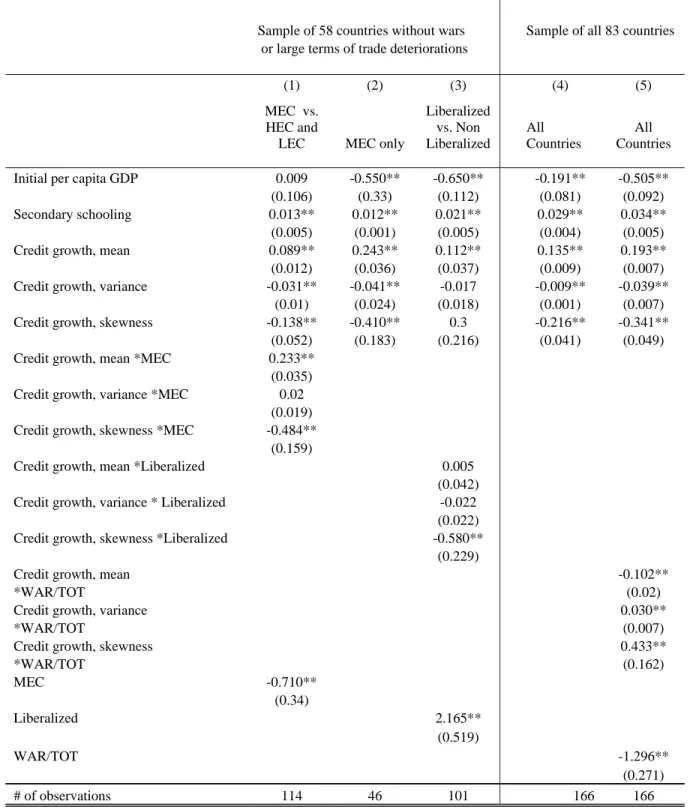
In order to capture more formally these differences, we add to our benchmark regression — column (2) in Table 1— an interaction dummy that equals one if a country is an MEC and zero otherwise. This dummy is interacted with the three moments of credit growth. Tables 4a and 4b show that, consistent with the prediction of the model, the effect of risk taking on growth is strongest across MEC countries. In that set a one unit reduction in skewness enhances growth by 1 6The system estimator corrects for the potential imprecision of the difference estimator. The estimation procedure
is valid only under the assumption of weak exogeneity of the explanatory variables. That is, they are assumed to be uncorrelated with future realizations of the error term.
0.622% and only by 0.138% in the other countries.17 Thisfinding means that the growth enhancing effect of systemic risk is more than three times higher in MEC countries.18
The impact of variance on growth does not seem to differ between MECs and other countries, as the interaction dummy for variance is not significant. Meanwhile, the effect of mean credit growth is substantially more important in MECs. It is more than three times as high in MECs than in other countries.
We would like to emphasize that the negative link between skewness and growth remains sig-nificant and quantitatively similar when we run the regression only with the MEC set, as shown in column (2). This shows that the link between negative skewness and growth is not driven by the difference between country groups. There exists a trade-offbetween smoothness and growth across the MEC set, as illustrated by the example of India and Thailand above.
Financial liberalization
As we have discussed, the mechanism that links growth to crises requires not only weak insti-tutions, but also policy measures that are conductive to the emergence of systemic risk. Financial liberalization can be viewed as such a policy measure. In non-liberalized economies, regulations do not permit agents to take on significant risk.
To capture the fact that the interaction of weak institutions with liberalization is key, we classify our data in country-years that are liberalized and those that are not liberalized. Table 3 shows that negative skewness as well as high mean growth rates are associated with financial liberalization. This indicates that in the presence of weak institutions, liberalization has facilitated systemic risk taking and has led to both higher mean credit growth and occasional crises.
To capture this difference more formally we introduce a liberalization dummy that equals one for decades in which a country was liberalized, and zero for decades in which it was not.19,20 Tables 4a and 4b show a significant difference in the effect of skewness between liberalized and not liberalized countries. In non-liberalized countries, the skewness coefficient is positive and insignificant, while in liberalized countries it is negative and significant. This suggests that the risk-taking mechanism 1 7The estimate 0.622% is the sum of the coefficient on skewness and that on skewness interacted with the MEC
dummy.
1 8
As a robustness check we use an income per-capita threshold —$17,500 in 2000— to define the HEC set. With the exception of three countries, the countries selected are the same as those selected by the rule of law criterion. Sign and significance levels remain the same, and point estimates are very similar.
1 9See the appendix for a description of how the liberalization index is constructed. 2 0
Country-decades where there was a transition from closed to open were dropped from this regression. Fifteen observations where dropped from the sample in this way.
we described is present only in liberalized economies. We can also see in column (3) of Table 4a that the liberalization dummy enters positively and is significant. This indicates that the effect of skewness is independent of other effects that liberalization might have on growth through other channels.21
Wars and terms of trade deteriorations
We should not expect the negative link between skewness and growth to exist when skewness is generated by wars or terms of trade deteriorations. These shocks are exogenous and do not reflect the relaxation offinancial bottlenecks induced by systemic risk. Nevertheless, to investigate whether the effect of negative skewness on growth is observed in an unconditional sample, we estimate the panel regression including all 83 countries for which we have available data. Column (4) in Table 4a shows that indeed skewness enters negatively and remains statistically significant, although the magnitude of the point estimate is reduced from -0.302 to -0.216.
In column (5), we include an interaction dummy that equals one for countries that have expe-rienced either wars or large terms of trade deteriorations. As expected, the negative link between skewness and growth is reversed for this set of countries.22
2.3
Instrumental Variables Estimation
In our model economy, the risk-taking mechanism that generates skewness is exogenous to growth.23 Thus, there is no reverse causality from mean growth to the asymmetric shape of the credit growth distribution. Nevertheless, in order to overcome potential remaining endogeneity we use an index of financial liberalization to instrument for skewness. In the presence of contract enforceability prob-lems,financial liberalization permits the undertaking of systemic risk, which both relaxes borrowing constraints and leads to occasional crises. Thus, in our model economy financial liberalization is correlated with negative skewness, but it does not have another independent effect on growth, making it an appropriate instrument.
Column (1) in Table 5 displays the estimates of the second stage of a two-stage least squares 2 1
For an extensive empirical treatment offinancial liberalization dummies in growth regressions see Beckaert, et.al. (2004).
2 2The sum of the coefficient on skewness and that on skewness interacted with the dummy is positive and statistically
significant. A Wald test indicates that this sum is statistically significant.
2 3
Risk taking allows agents to attain greater leverage, which increases investment and growth. Risk taking, however, also implies that crises will occur occasionally. Since there is no reversed impact of growth on crisis, there is also no causal impact of growth on skewness, making skewness a valid right hand side variable.
regression. We can see that skewness is statistically significant and has a point estimate which is even greater than the one from our benchmark regression. Furthermore, the mean remains sig-nificant and of similar magnitude, but variance is no longer statistically sigsig-nificant. Column (3) shows that in thefirst stage, there is a significant negative link betweenfinancial liberalization and skewness.24 The result in the first stage is consistent with the well documented fact that financial liberalization has been followed by boom-bust cycles.25
Regressions (1) and (3) estimated by GMM are given in column (2) (second stage) and (4) (first stage). They lead to qualitatively similar results as the two-stage least squares regression.
Finally, we acknowledge that there may be other independent channels through whichfinancial liberalization affects growth that we have not accounted for in the model. We are nevertheless confident that favouring the emergence of systemic risk is a important channel through which financial liberalization can affect growth.
2.4
Robustness
Here, we show that the negative link between skewness and growth is robust to the elimination of extreme observations, to the introduction of more control variables, and to alternative specifications of the panel regression.
There are no statistical outliers in our regressions in the sense that a country’s residual devi-ates by more than two standard deviations from the mean. Nevertheless, to see whether extreme observations have an influence on our results we exclude, from our benchmark panel-regression, the countries with the three largest and three lowest residuals both individually and collectively. The countries with the largest positive residuals are China, Korea and Botswana. Those with the most negative residuals are Jordan, Niger and Papua New Guinea. As Table 6 shows, the exclusion of these extreme observations does not change our results. In particular, the coefficient on skewness is negative and significant at the 5% level. The point estimates range between−0.24 and −0.32, which are quite similar to our benchmark estimate of −0.30.
In Table 7 we add to our benchmark regression several control variables commonly used in the empirical growth literature: the government share in GDP, life expectancy, inflation and the terms of trade growth. The addition of these variables does not impact the estimates of the three moments of credit growth.
2 4
However, as the F-statistic has only a value of 5.02, it must be considered only a weak instrument according to the standard reference value of 10 in the literature.
Table 8a shows that our benchmark panel regression provides qualitatively the same results when estimated with fixed effects, random effects and time effects. Table 8b shows that this robustness also largely exists in the full set of 83 countries. The only exception is that skewness is not statistically significant in the random effects model.
In sum, ourfindings show that countries that followed a risky credit path have on average grown faster than countries with stable credit conditions. These resultsdo not imply that crises are good for growth. They say that undertaking credit risk has led to higher growth, but as a side-effect, it has also led tooccasional crises. This link between skewness and growth is robust and quite stable across alternative sets of countries and specifications. Furthermore, this effect is independent of the negative effect of variance and growth.
3
Model
Here, we formalize the argument presented in the Introduction and show that it is internally consistent. The link between growth and propensity to crisis derives from the fact that risk taking allows financially constrained firms attain greater leverage. Furthermore, the model allows us to determine when systemic risk is growth enhancing and when it is socially efficient.
We consider an ‘Ak’ growth model with uncertainty. During each period the economy can be either in a good state (Ωt = 1), with probability u, or in a bad state (Ωt = 0). To allow for the endogeneity of systemic risk we assume that there are two production technologies: a safe and a risky. Under the safe technology, production is perfectly uncorrelated with the state, while under the risky one the correlation is perfect. For concreteness, we assume that the risky technology has a return Ωt+1θ,and the safe return is σ
qtsaf e+1 =σIts, qriskyt+1 = ⎧ ⎨ ⎩ θItr prob u, u∈(0,1) 0 prob 1−u (2)
whereIts is the investment in the safe technology and Itr is the investment in the risky one.26 Production is carried out by a continuum of firms with measure one. The investable funds of a firm consist of its cashflowwtplus the one-period debt it issuesbt.Since thefirm promises to repay next period bt[1 +ρt],thefirm’s time t budget constraint and timet+ 1profits are, respectively
wt+bt = Its+Itr (3)
πt+1 = max{qt+1−bt[1 +ρt], 0} (4)
2 6
The debt issued by firms is acquired by international investors that are competitive risk-neutral agents with an opportunity cost equal to the international interest rate1 +r.
In order to generate both borrowing constraints and systemic risk we follow Schneider and Tornell (2004) and assume that firmfinancing is subject to two credit market imperfections: con-tract enforceability problems and systemic bailout guarantees. We model the first imperfection by assuming that firms are run by overlapping generations of managers who live for two periods and cannot commit to repay debt. In thefirst period of her life, a manager makes investment and diversion decisions. In the second period of her life she receives a shareeof profits and consumes. For concreteness, we make the following assumption.
Contract Enforceability Problems. If at time t the manager incurs a non-pecuniary cost h·e·[wt+bt],then att+ 1thefirm will be able to divert all the returns provided it is solvent. The representative manager’s goal is to maximize next period’s expected payoffnet of diversion costs. We model the second imperfection by introducing an agency that grants bailouts when there is a systemic default, but not when there is an idiosyncractic default.
Systemic Bailout Guarantees. The bailout agency pays lenders the outstanding debts of all defaulting firms if and only if a majority of firms becomes insolvent (i.e.,πt≤0).
Bailouts are financed by taxing the consumers, who own the firms. Consumers are infinitely lived, and can borrow and lend at the world interest rate. During every period the representative consumer receives dividends from firms, pays taxes, and consumes. Thus, he solves the following problem max {cj}∞ j=0 Et ∞ X j=0 δt+jv(ct+j), s.t. Et ∞ X j=0 δt+j[dt+j−ct+j −τt+j] ≥0, δ := 1 1 +r We impose the condition that the sequence of taxes is such that the bailout agency breaks even
E0P∞j=0δj
©
[1−ξj+1][bj[1 +ρj+1] +aj+1]−τj+1
ª
= 0, (5)
whereξt+1= 1ifπt+1>0, and zero otherwise.
Since guarantees are systemic, the decisions of managers are interdependent and are determined in the following credit market game. During each period, every young manager proposes a plan Pt= (Itr, Its, bt,ρt) that satisfies budget constraint (3). Lenders then decide whether to fund these plans. Finally, young managers make investment and diversion decisions.
If the firm is solvent att+ 1 (πt+1 >0)and no diversion scheme is in place, the old manager
receiveseπt+1and consumers receive a dividenddt+1= [d−e]πt+1. In contrast, if thefirm is solvent
and there is diversion, the old manager getseqt+1, consumers get[d−e]qt+1and lenders receive the
bailout if any is granted. Finally, under insolvency consumers and old managers get nothing, while lenders receive the bailout if any is granted. The problem of a young manager is then to choose an investment planPtand a diversion strategy ηt to solve:
max
Pt,ηt Etξt+1{[1−ηt]πt+1 + ηt[qt+1−h[wt+bt]]}e s.t. (3),
whereηt= 1if the manager has set up a diversion scheme, and zero otherwise, andξt+1 is defined in (5).
To sharpen the argument we assume that crises have very steep costs: in case of insolvency all output is lost in bankruptcy procedures. In order to restart the economy in the wake of a systemic crisis we assume that if afirm is insolvent, it receives an aid payment from the bailout agency (at) that can be arbitrarily small. Thus, afirm’s cash-flow evolves according to
wt= ⎧ ⎨ ⎩ [1−d]πt if πt>0 at otherwise (6)
To close the model we assume that in the initial period cashflow isw0= [1−d]w−1,dividends are
d0= [d−e]w−1 and the old managers’ payment is ew−1.
3.1
Discussion of the Setup
We have considered a very stylized model to capture the essential features of the mechanism through which policies that permit systemic risk taking lead to faster growth in economies where weak in-stitutions give rise borrowing constraints. An attractive feature of this setup is that the mechanism is transparent and the results depend on just two parameters: the degree of contract enforceability h,and the likelihood of crisis 1−ut+1.
In our setup there are two states of nature and agents’ choice of production technology de-termines whether or not systemic risk arises. This setup is meant to capture more complicated situations, like for instance, the oft-cited phenomenon of currency mismatch whereby systemic risk is endogenously generated through risky debt denomination.
To make clear that the positive link between growth and systemic risk in our mechanism does
restrict the risky technology to have alower expected return (uθ) than the safe one
1 +r≤uθ<σ<θ (7)
Two comments are in order. First, the condition uθ < σ implies that the moral hazard induced by the guarantees supports lending to inefficient projects. Nevertheless, due to the leverage effect, an equilibrium with risky projects can be socially efficient —as shown by Proposition 4.1. Second, in our simple set-up relaxing 1 +r ≤uθ could lead to growth-enhancing systemic risk, but such an equilibrium would be socially inefficient. This condition could be relaxed in a more compli-cated set-up with externalities. For instance, in the two-sector framework of Ranciere, Tornell and Westermann (2003), greater leverage in the constrained sector has a positive externality on the unconstrained sector.
The mechanism that links growth and the propensity to crisis requires that both borrowing constraints and systemic risk arise simultaneously in equilibrium. In most of the literature there are models with either borrowing constraints or excess risk, but not both. As Schneider and Tornell (2004) show, in order to have both borrowing constraints and risk-taking, enforceability problems must interact with systemic guarantees. If only enforceability problems were present, agents would be overly cautious and the equilibrium would feature borrowing constraints, but no risk taking. If only guarantees were present, there would be no borrowing constraints and risk-taking would not be growth enhancing.
Notice that the two distortions act in opposite directions, and in general, neutralize each other. Propositions 3.1-4.1 demonstrate that systemic risk is growth enhancing and socially efficient only when institutions are weak, but not too weak. In our setup countries with weak institutions have a low level of contract enforceability h. More specifically we will assume throughout the paper that enforceability problems are ‘severe’
0≤h < u[1 +r] (8)
This condition is necessary for borrowing constraints to arise in equilibrium. Lenders are willing to lend up the point where borrowers do not find it optimal to divert. If (8) did not hold, the expected debt repayment in a risky equilibrium would be lower than the diversion cost h[wt+bt] for all levels ofbt.Thus, lenders would be willing to lend any amount.
We have assumed that guarantees are systemic. If instead institutions were so weak that bailouts were granted whenever there was an individual default, borrowing constraints would not arise because lenders would always be repaid (by taxpayers).
Our setup makes it difficult to prove that systemic risk is growth enhancing and socially efficient. First, we have assumed that there are 100% bankruptcy costs (in case of a crisis all output is lost). Second, in the wake of crisis cash-flow offirms collapses (it equals the tiny aid paymentat).Since the production technology is linear, this collapse in cash-flow reduces the level of output permanently. Consumers do not play a central role. They are simply a device to transfer fiscal resources from firms to the bailout agency. We will use the consumers to show that the fiscal costs of the guarantees can be lower than the benefits. The assumption that consumers can borrow and lend at the world interest rate can be relaxed if we assume instead that the bailout agency has access to an international lender of last resort. In this case the bailout agency would repay the international loan from taxes levied in good times.
3.2
Equilibrium Risk Taking
In this subsection, we characterize the conditions under which borrowing constraints and systemic risk can arise simultaneously in a symmetric equilibrium.
Let us define asystemic crisis as a situation where a majority offirms go bust, and let us denote the probability that this event occurs next period by 1−ut+1. Then, a plan(Itr, Its, bt,ρt) is part of a symmetric equilibrium if it solves the representative manager’s problem, taking ut+1 and wt as given.
The next proposition characterizes symmetric equilibria at a point in time. It makes three key points. First, binding borrowing constraints arise in equilibrium only if contract enforceability problems are severe (h <¯h). In this case afinancial bottlenecks arises as investment is constrained by cashflow. Second, systemic risk taking eases, but does not eliminate, borrowing constraints and allowsfirms to invest more than under perfect hedging. This is because systemic risk taking allows agents to exploit the subsidy implicit in the guarantees via a lower expected cost of capital. Third, systemic risk may arise endogenously only if bailout guarantees are present. Guarantees, however, are not enough. It is also necessary that a majority of agents coordinate in taking on risk, and that contract enforceability problems are not ‘too severe’ (h>h). If h were too small, taking on risk would not pay because the increase in leverage would be too small.
Proposition 3.1 (Symmetric Credit Market Equilibria (CME)) Borrowing constraints arise if and only if the degree of contract enforceability is not too high: h < ut+1δ−1. If this condition
holds, credit and investment are
bt= [mt−1]wt, Itr+Its=mtwt, with mt= 1
1−u−t+11hδ. (9) • There always exists a ‘safe’ CME in which all firms only invest in the safe technology and a
systemic crisis next period cannot occur: ut+1 = 1.
• There also exists a ‘risky’ CME in which ut+1 = u and all firms only invest in the risky
technology if and only if h > h(u), where h(u) is given by (18).
The intuition is the following. Given that all other managers choose a safe plan, a manager knows that no bailout will be granted next period. Since the expected return of the safe technology is greater than that of the risky technology (i.e., σ > uθ), she will choose a safe plan. Since the firm will not go bankrupt in any state and lenders must break even, the interest rate that the manager has to offer satisfies 1 +ρt = 1 +r. It follows that lenders will be willing to lend up to an amount that makes the no diversion constraint binding: (1 +r)bt≤h(wt+bt).By substituting this borrowing constraint in the budget constraint we can see that there is a financial bottleneck: investment equals cash-flow times a multiplier (Its=mswt, wherems = (1−hδ)−1).27
Consider now the risky equilibrium. Given that all other managers choose a risky plan, a young manager expects a bailout in the bad state, but not in the good state. Since lenders will get repaid in full in both states, the interest rate that allows lenders to break-even is again 1 +ρt = 1 +r. It follows that the benefits of a risky plan derive from the fact that, from the firm’s perspective, expected debt repayments are reduced from1 +r to[1 +r]u,as the bailout agency will repay debt in the bad state. A lower cost of capital eases the borrowing constraint as lenders will lend up to an amount that equatesu[1 +r]bttoh[wt+bt].Thus, investment is higher than in a safe plan. The downside of a risky plan is that it entails a probability1−uof insolvency. Will the two benefits of a risky plan —more and cheaper funding— be large enough to compensate for the cost of bankruptcy in the bad state? Ifh is sufficiently high, expected profits under a risky plan exceed those under a safe plan: uπrt+1 >πst+1.
2 7This is a standard result in the macroeconomics literature on credit market imperfections —e.g. Bernanke et. al.
3.3
Long Run Growth
We have loaded the dice against finding a positive link between growth and systemic risk. First, we have restricted the expected return on the risky technology to be lower than the safe return (θu <σ). Second, we have allowed crises to have largefinancial distress costs as cash-flow collapses in the wake of crisis and the aid payment (at) can be arbitrarily small. Since the production technology is linear, this fall in cash-flow reduces the level of output permanently: crises have long-run effects.
Here we investigate whether, in the presence of borrowing constraints, systemic risk can be growth-enhancing by comparing two symmetric equilibria: safe and risky. In a safe(risky) equi-librium every period agents choose the safe(risky) plan characterized in Proposition 3.1. We ask whether average long-run growth in a risky equilibrium is higher than in a safe equilibrium.
The answer to this question is not straightforward because an increase in the probability of crisis (1−ut+1) has opposing effects on long-run growth. One the one hand, a greater 1−ut+1
increases investment and growth along the lucky no-crisis path by increasing the subsidy implicit in the guarantee and allowing firms to be more leveraged. On the other hand, a greater1−ut+1
makes crises more frequent, which reduces average long-run growth.
In a safe symmetric equilibrium, crises never occur —i.e., ut+1 = 1 in every period. Thus, cash
flow dynamics are given by ws
t+1 = [1−d]πst+1, where profits are πst+1 = [σ−h]mswt. It follows that the long-run annual growth rate,gs,is given by
1 +gs = [1−d][σ−h]ms ms= 1
1−hδ (10)
Since σ > 1 +r, the lower h, the lower growth. Consider now a risky symmetric equilibrium. Since firms use the risky technology during every period t, there is a probability u that they will be solvent at t+ 1 and their cash-flow will be wt+1 = [1−d]πrt+1, whereπrt+1 = [θ−u−1h]mrwt.
However, with probability 1−u firms will be insolvent att+ 1 and their cashflow will equal the aid payment from the bailout agency: wt+1 =at+1.We parametrizeat+1 as follows
at+1 =α(1−d)(θ−u−1h)mrwt, α∈(0,1) (11)
The expression multiplying α is the cash-flow that the firm would have received had no crisis occurred. Clearly, the smallerα,the greater the financial distress costs of crises. Since crises can occur in consecutive periods, growth rates are independent and identically distributed over time.
Thus, the long-run mean annual growth rate is given by E(1 +gr) =uγn+ (1−u)γc, γ n= [1 −d][θ−u−1h]mr, mr= 1−u1−1hδ γc=αγn (12)
The following proposition compares the mean growth rates in (10) and (12).
Proposition 3.2 (Long-run Growth) Consider an economy where crises have arbitrarily large financial distress costs (α→0).
• Systemic risk arises in equilibrium and increases average long-run growth if and only if con-tract enforceability problems are severe, but not too severe: h∈(h, uδ−1), whereh is uniquely defined by (18).
• The greaterh,within the range (h, uδ−1),the greater the growth enhancing effects of systemic risk.
A shift from a safe to a risky equilibrium increases the likelihood of crisis from 0to1−u.This shift results in greater leverage (brt
wt − bs
t wt = m
r
−ms), which increases investment and growth in periods without crisis. This is the leverage effect. However, this shift also increases the frequency of crises and the associated collapse in cash flow and investment, which is bad for growth. This proposition states that the leverage effect dominates the crisis effect if the degree of contract enforceability is high enough, but not too high. If h is high enough, the undertaking of systemic risk translates into a large increase in leverage, which compensates for the potential losses caused by crises. If h were excessively high, there would be no borrowing constraints to begin with and risk taking would not enhance growth.
An increase in the degree of contract enforceability —a greater h within the range (h, uδ−1)— leads to higher profits and growth in both risky and safe economies. An increase inh can be seen as a relaxation of financial bottlenecks that allows greater leverage in both economies. However, such an institutional improvement benefits more the risky economy as the subsidy implicit in the guarantee amplifies the effect of better contract enforceability.
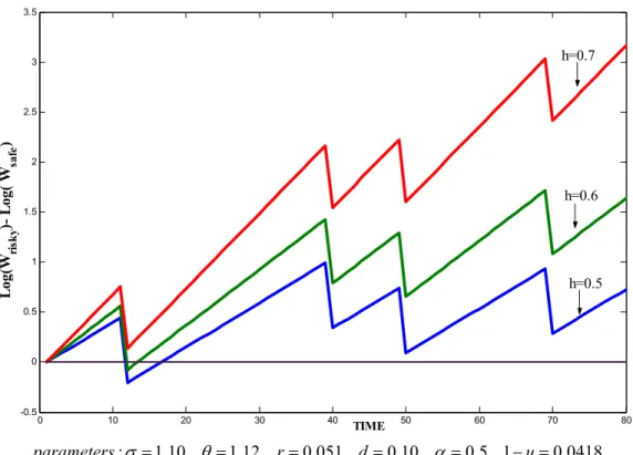
Notice that the thresholdhin Propositions 3.1 and 3.2 is the same. This implies that whenever risk taking is individually optimal it is also growth enhancing. Observe, however, that systemic risk and higher growth need not be socially efficient. We will come back to this issue in Section 4. Figure 4 illustrates the limit distribution of growth rates by plotting different paths ofwt corre-sponding to different realizations of the risky growth process. Thisfigure makes clear that greater
long-run growth comes at the cost of occasional busts. We can see that over the long-run most of the risky paths outperform the safe path, except for a few unlucky risky paths. If we increased the number of paths, the cross section distribution would converge to the limit distribution.
The choice of parameters used in the simulation depicted in Figure 4 is detailed in Appendix B. The probability of crisis (4.18%) corresponds to the historical probability of falling into a systemic banking crisis in our sample of countries over 1980-2000. The financial distress costs are set to 50%, which is a third more severe than our empirical estimate derived from the growth differential between tranquil times and a banking crisis. The degree of contract enforceability is set just above the level necessary for risk-taking to be optimal (h =0.5). Finally, the mean return on the risky technology is 2% below the safe return. Nevertheless, growth in the risky equilibrium is on average 3% higher than in the safe equilibrium.
Figure 5 plots the difference in logwtof risky and safe economies for varying degrees of contract enforceability. As we can see, an increase in the degree of contract enforceability increases the growth benefits from risk taking. Figure 6 plots the difference in log wt for different financial distress costs. Recall that if risk-taking is optimal, it is also growth enhancing for any arbitrarily largefinancial distress cost. Less severe distress costs evidently improve the average long-run growth in the risky equilibrium. Notice that the upper curve is computed with the value offinancial distress costs estimated from our sample of 83 countries over 1980-2000 (α= 0.8).
3.4
From Model to Data
The equilibrium of the model implies a negative link between skewness and growth, and it identifies the set of countries over which our mechanism is at work. We consider each in turn.
Skewness and Growth
In a risky equilibrium,firms face endogenous borrowing constraints, and so credit is constrained by cash flow. Since along a no-crisis path cash flow accumulates gradually, credit grows fast but
only gradually. In contrast, when a crisis erupts there are widespread bankruptcies, cash flow
collapses and credit falls abruptly. The upshot is that in a risky equilibrium the growth rate can take on two values: low in the crisis state (gc), or high in the lucky no crisis state (gn).
Empirically, financial crises are rare events.28 In terms of the model, this fact means that the probability of the bad state1−uis rather small, and in particular less than a half. This implies that the low growth rate realizations (gc) are farther away from the mean than the high realizations
2 8
(gn). Thus, in a long enough sample, the distribution of growth rates in a risky equilibrium is characterized by negative outliers and is negatively skewed. In contrast, in the safe equilibrium there is no skewness as there is no uncertainty in the growth process.29 Since risk taking is optimal whenever it is growth enhancing (by Propositions 3.1 and 3.2), it follows that there is a negative link between mean long-run growth and skewness.
Quality of Institutions and Policy Environment
Our argument has two empirical implications that underlie the country grouping criterion and the instrument selection in Section 2. First, our model predicts that on average we should observe a stronger link between systemic risk and higher long-run growth in countries with a middle degree of institutional quality than in other groups of countries. Second, our model predicts that this link should be stronger in the set offinancially liberalized countries.
The model emphasizes two key aspects of the quality of institutions. The first aspect has to do with the degree of contract enforceability h. On the one hand, borrowing constraints arise in equilibrium only if contract enforceability problems are ‘severe’: h <¯h.Otherwise, borrowers would alwaysfind it profitable to repay debt. On the other hand, risk taking is individually optimal and systemic risk is growth enhancing only if h > h. Only if h is large enough can risk taking induce a big enough increase in leverage to compensate for the distress costs of crises. It follows that a positive link between systemic risk and long-run growth exists only in the set of countries where contract enforceability problems are severe, but not too severe: h∈(h,¯h).
The second aspect of the quality of institutions is the generosity of the guarantees. If institutions
are so weak that a bailout is granted whenever there is an isolated default —because authorities
cannot withstand the political or corruption pressures, the mechanism does not work. Instead, there would be a collusion between politically connected lenders and borrowers to run andfinance unproductive projects and extract taxpayers’ money through bailout guarantees.30 Institutions
must be sufficiently strong so that bailouts are granted only in case of a systemic crisis.31
Consider next the policy environment. The moderately weak institution framework we have described above is not sufficient to generate systemic risk. Proposition 3.1 implies that the presence 2 9In this argument we have used the fact that in our setup two crises can occur in consecutive periods. However, a
similar argument could be made if a crisis were followed by a recovery during which another crisis could not happen (see Ranciere, Tornell and Westermann (2003)). In that setup no-crisis times are more frequent that crisis times.
3 0
This phenonenon has been described by Faccio (2004) and Khawaja and Mian (2004).
3 1If the decision tofinance the guarantees involved an international financial institution, its monitoring capacity
of policies that liberalize financial markets and allow agents to take on systemic risk is necessary. The key for the risk-growth link is the combination of moderately weak institutions withfinancial liberalization.
4
Financing of the Guarantees
The existence of systemic risk and high average growth rates depend on systemic guarantees, which are funded domestically via lump-sum taxes on consumers. Here, we consider an economy with severe contract enforceability problems, and ask whether the expected value of the dividend stream net of taxes is greater in a risky than in a safe equilibrium. That is, we ask whether taxpayers will be made strictly better off by financing the bailout guarantees. By fully accounting for the costs and benefits associated with thefinancing of the guarantees, we can assess when systemic risk is not only growth enhancing, but also socially efficient. Notice that our setup is biased against the efficiency of guarantees: the risky technology is restricted to have a lower expected return than the safe technology, there is no externality associated with higher investment, and during a crisis all output is lost in bankruptcy procedures and cash-flow collapses. This means that all the social gains from risk taking come from the ability to attain greater leverage.
To simplify notation we set, without loss of generality, the interest rate r to zero.32 Thus, the expected present value of the representative consumer’s net income is
Y =E0
X∞
j=0[dj−τj], (13)
where the dividend dj equals [d−e]πj in periods without a crisis and zero otherwise, and the sequence of taxes{τj}satisfies the bailout agency’s break-even constraint (5). In a safe equilibrium taxes are always zero because insolvencies never occur. Since during every period t≥1profits are πsj = [σ−h]mswj−1 and initiallyd0 = [d−e]w−1 andw0 = [1−d]w−1, in the safe equilibrium (13)
becomes Ys=X∞ j=0[d−e]wj−1 = d−e 1−γsw−1, γ s= 1 +gs (14)
Consider next the risky equilibrium. When a crisis erupts the bailout agency pays lenders the debt they were promised(bj−1)and givesfirms a small amount of seed money (aj).To ensure that the bailout agency breaks even consider a tax sequence in which, during each period, taxes equal the bailout payments. This sequence is feasible because taxpayers have access to completefinancial
markets. It follows that the expected present value of the taxpayer’s net income is Yr = E0 ∞ X j=0 © [d−e]πrjξj−[bj−1+aj][1−ξj] ª (15) = d−e[1−(1−u)αγ n] −[1−u][(mr−1)(1−d) +αγn] 1−γr w−1, γ r= [u+ (1 −u)α]γn
whereξj = 0if there is a crisis at timej.Thefirst two terms in the numerator represent the average dividend, while the third term represents the average tax, which covers the seed money given to firmsαγnwt−1 and the debt that has to be repaid to lenders. The latter equals the leverage times
the reinvestment rate bt−1
wt−1
wt−1
πt−1wt−1 = (m
r
−1)(1−d)wt−1.33
The next proposition states that if enforceability problems are not too severe, the fiscal costs of crises are outweighed by the benefits of greater growth.
Proposition 4.1 (Financing the Guarantees and Social Efficiency) If the manager’s pay-out rate e is small enough, there exists a unique threshold for the degree of contract enforceability
h∗∗< u, such that the expected present value of taxpayers’ net income is greater in a risky economy than in a safe one for any aid policyα∈(0,1)if and only if h > h∗∗.
To get further insight into social efficiency consider the excess social return of firms when the manager’s shareetends to zero. Rewrite (14) and (15) as follows
Ys−w−1 = (1−d)(σ−1)ms w−1 1−γs = (1−d)(σ−1) ∞ X t=0 Its Yr−w−1 = (1−d)(uθ−1)mr w−1 1−γr = (1−d)(uθ−1)E0 ∞ X t=0 Itr
We can interpret Yi−w−1 =Rimi w1−−γ1i as the expected excess social return of afirm. This excess return has three components: the static return (Ri);the leverage (mi−1); and the mean growth rate of cash-flow (γi). Since we have imposed the condition uθ<σ, the following trade-offarises. Projects have a higher rate of return in a safe economy that in a risky one (Rs> Rr), but leverage and scale are smaller (ms < mr). In a risky economy, the subsidy implicit in the guarantees attracts projects with a lower return but permits greater scale by relaxing borrowing constraints. This relaxation of thefinancial bottleneck is dynamically propagated (γr>γs). Ifhis high enough, greater leverage and growth compensate for the costs of crises. Thus, when contract enforceability
3 3The term
−e[1−(1−u)αγn]w
t−1reflects the fact that during no crisis times the old manager gets a shareeofwt,
problems are of limited severity, the excess return in the risky economy is greater than in the safe economy.
Is systemic risk socially efficient whenever it is growth enhancing? The answer is no. When financial crises are very costly, social efficiency depends on our measure of the weakness of institu-tions, as the next Corollary shows.
Corollary 4.1 (Growth vs. Efficiency) If crises have large distress costs, the social efficiency threshold h∗∗ is greater than the risk-taking (and growth-enhancing) threshold h. In this case sys-temic risk is growth enhancing but socially inefficient if h∈(h, h∗∗).
We have seen that systemic risk is growth enhancing whenever it is individually optimal (Propo-sitions 3.1 and 3.2). When the financial distress costs of crises are large, there is a range for the degree of contract enforceability in which risk taking is individually optimal (h > h), but not so-cially efficient (h < h∗∗).Whenh∈(h, h∗∗)the leverage gains obtained byfirms are big enough to justify individual risk-taking, but are not big enough to compensate for the social costs offinancial crises.
The reason for this gap is the following. The social cost of borrowing is identical in safe and risky economies. However, while in the former the individual firm internalizes 100% of the debt costs, in a risky economy the individual firm internalizes only a share u of the debt costs and taxpayers cover the rest. As a result, risk taking might be individually optimal, even if it is not socially efficient. To see when this is the case consider the ratio of excess social returns
Yr−w−1 Ys−w −1 = Eπ r πs ·k, k:= uθ−1 σ−1 σ−h uθ−h
The k ratio is smaller than one because σ > θu and h < u. Since at the threshold h expected profits in both economies are equal (Eπr = πs), the social return is greater in the safe economy. The leverage effect implies that Eπr grows faster withh than πs.Hence, when h is high enough the risky-safe leverage gap more than compensates for the social cost of crises and Yr> Ys.
We want to emphasize that our results do not imply that guarantees are always socially efficient. In addition to Corollary 4.1, we have seen that in the absence of a mechanism to relax borrowing constraints, bailout guarantees are unambiguously bad. This occurs if either h is too high, so that borrowing constraints do not arise, or h is too low, so that there is no significant increase in leverage.34
The funding of the guarantees can be interpreted as a redistribution from the financially un-constrained to the financially constrained agents in the economy. On the one hand, taxpayers benefit from the guarantees because higher mean growth means higher dividend growth. On the other hand, taxpayers bear thefiscal costs associated with the risk taking that permits constrained agents to exploit the subsidy implicit in the guarantees.
5
Related Literature
Most of the empirical literature onfinancial liberalization and economic performance focuses either on growth or onfinancial fragility and excess volatility. Beckaert, Harvey and Lundblad (2004)find a robust and economically important link between stock market liberalization and growth, while Henry (2002) finds similar evidence by focusing on private investment.35 Kaminsky and Reinhart (1998) and Kaminsky and Schmukler (2002) show that the propensity to crises and stock market volatility increase in the aftermath offinancial liberalization. Our findings help to integrate these contrasting views.
A novelty of this paper is to use skewness to analyze economic growth. In thefinance literature, skewness of stock market returns plays an important role —e.g., Beckaert and Harvey (1997), Kraus and Litzenberger (1976), Harvey and Siddique (2000) and Veldkamp (2004). This paper borrows from the finance literature the idea that variance is not sufficient to characterize risk when the distribution of stock returns is asymmetric.
In our empirical analysis, the negative link between skewness and growth coexists with the negative link between variance and growth identified by Ramey and Ramey (1995). The contrasting growth effects of different sources of risk are also present in Imbs (2004), whofinds that aggregate volatility is bad for growth, while sectorial volatility is good for growth.
A key result of this paper is that a bailout policy that discourages hedging can be efficient as it induces a redistribution from non-constrained to constrained agents. Tirole (2003) and Tirole and Pathak (2004) reach a similar conclusion in a different set up. In their framework, a country pegs the exchange rate as a means to signal a strong currency and attract foreign capital. Thus, it must discourage hedging and withstand speculative attacks in order for the signal to be credible.
By focusing on the growth consequences of imperfect contract enforceability, this paper is con-nected with the growth and institutions literature pioneered by North (1981). For instance, Ace-3 5In contrast, the evidence on the link between capital account liberalization and growth is mixed. See Eichengreen
moglu et.al. (2003) show that better institutions lead to higher growth, lower variance and less frequent crises. In our model, better institutions also lead to higher growth, and it is never optimal for countries with strong institutions to undertake systemic risk. Our contribution is to show how systemic risk can enhance growth by counteracting the financial bottlenecks generated by weak institutions.
Obstfeld (1994) demonstrates that financial openness increases growth if international risk-sharing allows agents to shift from safe to risky projects. In our framework, the growth gains are obtained by letting firms take on more risk and attain greater leverage.
The cycles in this paper are different from schumpeterian cycles in which the adoption of new technologies and the cleansing effect of recessions play a key role —e.g., Aghion and Saint Paul (1998), Caballero and Hammour (1994) and Schumpeter (1934). Our cycles resemble Juglar’s credit cycles in which financial bottlenecks play a dominant role. Juglar (1862, 1863) characterized asymmetric credit cycles along with the periodic occurrence of crises in France, England, and United States during the nineteen century.
Our model is related to Ranciere, Tornell and Westermann (2003) who consider two productive sectors: a tradables sector with access to international financial markets that uses inputs from the constrained nontradables sector. Greater investment by the latter benefits the former through cheaper inputs. That paper uses the framework of Schneider and Tornell (2004) to generate systemic risk via currency mismatch. It also generates several of the stylized facts associated with recent boom-bust cycles. The present one-sector model is not designed to generate such stylized facts. The gain is that the link between systemic risk and growth is transparent.
The growth enhancing effect of systemic risk shares some similarities with the role of bubbles in Olivier (2000) and Ventura (2004). In these papers, bubbles can foster growth by encouraging investment. The idea that introducing a new distortion counteracts the effects of an existing dis-tortion is also present in our approach as systemic guarantees relaxfinancial bottlenecks. However, our results do not exploit any form of dynamic inefficiency and our risky equilibria are sustainable over the infinite horizon. Finally, the mechanism we present is reminiscent of the literature on risk as a factor of production as Sinn (1986) and Konrad (1992).
6
Conclusions
We have found a robust link between systemic risk and growth: fast growing countries tend to experience occasional crises. In order to uncover this link it is essential to distinguish booms