Abstract: Key Words: Documentos Técnico-Científicos

n

Documentos Técnico-Científicos

C

C

o

o

m

m

m

m

o

o

m

m

E

E

c

c

o

o

n

n

o

o

m

m

i

i

c

c

C

C

y

y

c

c

l

l

e

e

s

s

i

i

n

n

B

B

r

r

a

a

z

z

i

i

l

l

’

’

s

s

N

N

o

o

r

r

t

t

h

h

e

e

a

a

s

s

t

t

Marcos Costa Holanda

Professor Titular do Departamento de Economia Aplicada e do Curso de Mestrado em Economia da Universidade Federal do Ceará (Caen-UFC)

André Matos Magalhães

Professor Assistente do Departamento de Econo-mia da Universidade Federal de Pernambuco (UFPE)

Abstract:

Most of the debate on promoting regional economic development in the Northeast of Brazil has been concentrated on the effects that national economic policies would have in the region. Little attention has been given, however, to the analysis of the effects that an individual state economy could have in other states within the region. The paper performs an empirical study on the economic interaction of the three largest economies of Brazilian Northeast: Bahia, Ceará, and Pernambuco. The empirical investigation is based on the estimation of a vector autoregression model (VAR) for the three states GSP (Gross State Product). The Information about the way that these three economies interact to each other can be obtained through the examination of the matrix of contemporaneous correlation of the residuals, Granger causality tests for blocks of equations, and examination of impulse response functions of the system.

Key Words:

National Policies; Regional Development; Economic Interaction; Regional Economy; Econometry; Quantitative Methods; Brazil-Northeast .

1 - INTRODUCTION

Most of the debate on promoting regional economic development in the Northeast of Brazil has been concentrated on the effects that national economic policies would have in the region. This stems from a belief that the region’s economies are strongly linked to the national economy, especially to the economies of more advanced states such as Sao Paulo and Rio de Janeiro. If that is the case a better understanding of such vertical interaction between the economies of the Northeast and those in the south would be essential to the definition of appropriated policies to face the economic underdevelopment of the region.

Little attention has been given, however, to the analysis of the effects that an individual state economy could have in others inside the region. Studies that try to analyze not the vertical economic interactions between the North and the South, but the horizontal economic interactions between the region’s state economies are not common in the literature. It can be the case that such studies would provide important information for the design of better economic policies for the region.

Contrary to a common view, it can be the case that the economies of the region are complementary rather than competitors to each other. It can also be the case that economic cycles in the region’s economies do not occur simultaneously or are even related to each other. An economic recovery in one state can be an isolated fact or it can mean future economic growth in others states.

The purpose of this paper is to perform an empir ical study on the economic interaction of the three largest economies of Brazilian Northeast. They are the economies of Bahia, Ceará, and Perna mbuco. It will be done in a very aggregated level, once it is based on the behavior of the Gross State Product (GSP). The analysis will focus on questions concerning the transmission and generation of economic cycles inside the region. We will investigate if the economic cycles are first generated, independently, in one state, and

then transmitted to the others or if they tend to occur contemporaneously due to common shocks. In case of transmitted shocks, it is important to verify the intensity and direction in which they occur.

The empirical investigation is based on the estimation of a Vector Autoregression model (VAR) for the three states GSP. The Information about the way that these three economies interact to each other can be obtained through the examination of the matrix of contemporaneous correlation of the residuals, Granger causality tests for blocks of equations, and examination of impulse response functions of the system.

Next section presents a short description of the VAR methodology. Section 3 presents the data and the main results of the VAR model. Section 4 concludes the paper.

2 - VECTOR AUTOREGRESSION

Vector Autoregression (VAR) methods, introduced and popularized by SIMS (1972, 1980b, 1980a, 1982), offer a simple way to deal multiequation systems that feature feedback effects among their variables. Its use has been widespread in macroeconomics.

In a structural form, a VAR with 2 variables and

one lagged value can be represented by1:

y

1t

=

b

10

−

b y

12 2t

+

γ

11

y

1t−1

+

γ

12

y

2t−1

+

ε

1t(1.a)

y2t =b20 −b y21 1t +γ 21y2t−1+γ22y2t−1+ε2t(1.b)

where

y

_1tand

y

_2t are stationary;

ε

_1t and

ε

_2t

are white noise disturbance with standard

deviation of

σ

₁ and

σ

₂, and individually serially

uncorrelated. So,

ε

_1t and

ε

_2t represent shocks

(pure innovations) to the sequences

y

_1tand

y

_2t.

The system embodies the feedback effect through

the presence of

y

_1t in the second equation and

y

_2t in the first one. If the coefficients

b

₁₂ and

1

In the example above the lag was arbitrarily set to one. In practice, however, a sufficiently number the

lags p are set in order to assure that the residuals are

b

₂₁ are not zero the shocks will have contemporaneous direct and indirect effects on the variable and the model cannot be directly estimated by Ordinary Least Square (OLS) because simultaneous equation bias (HAMILTON, 1994). However, if the model is estimated in the reduced form, such problem will not exist.

The reduced form can be found by manipulation of the equations in (1). Solving for the

y

_t

=

[

y

_1t

,

y

_2t

]

' vector in the left-hand side, and

defining

B

₁

=

[

b

₁₂

,

b

₂₁

]

'

B

₀

=

[

b

₁₀

,

b

₂₀

]

'

εε

t

=

[

t

,

t

]

'

ε ε

1 2













=

Γ

22 21 12 11

γ

γ

γ

γ

premultiplying the whole system by

Β

=

(

Ι

−

Β

₁

)

−1,

the resulting model is:

y

_t

=

A

₀

+

A y

_{1 t−1}

+

e

_t (2)

where,

A

₀

=

B B

−1 ₀,

A

₁

=

B

−1

Γ

Γ

and

e

_t

=

B

−1

εε

_t

The residuals, in the standard form VAR, have zero mean, constant variance and they are individually serially uncorrelated. The reduced model can be now estimated by (OLS) or

Maximum Likelihood (MLE)2. However, in

estimating the standard form of VAR, one must note that it is not possible to recover all the coefficients of the structural VAR without imposing some constraint on the coefficient of

matrix B3. It is worthy noticing that, even in its

reduced form, the VAR will contain a large number of parameters to be estimated. That can generate problems with the degrees of freedom and collinearity in the models that tend to make the forecasting performance of the VAR models seem poor (LESAGE & PAN, 1995).

2.1 - Granger causality test

2

If the lags are the same for all variables in each equa-tion, the OLS estimate is the ML estimate.

3

This stems from the fact that equation (1) contains more parameters than the reduced form is capable of estimating see ENDERS (1995).

One important issue in vector autoregression is whether or not a variable helps to forecast the others. GRANGER (1969) proposed a particular way to verify if such relationship exists.

According to his concept, if y does not help to

predict x, then it is said that y does not Granger

cause

x

. In this case, the Mean Square Error

(MSE) of a forecast of

x

_{t s+} using information on

x and y will be the same as the MSE when only

information on x is used.

In an n variable VAR with p lags, a sequence

y

_it

is said not Granger cause a sequence

y

_jt (for i≠j)

if and only if no lagged value of

y

_it enters in the

equation of

y

_jt. Note the concept refers only to

the lagged value, so it is possible for

y

_it to be

endogenous to

y

jt, even though it does Granger

cause the latter.

2.2 - Impulse response function

The VAR can also be represented in a Vector Moving Average (VMA) form. Considering as a

generalization of equation (2), a VAR with n

variable and p lags. Assuming that the conditions

for stability and stationarity hold, the VMA(∞)

representation is given by4: yt = + +µµ et ΨΨ1et−1+ΨΨ2et−2+ΨΨ3et−3+ ≡ +L µ Ψµ Ψ( )L et (3) where

µµ

=

(

I

n

−

A

1

−

A

2

−

−

A

p

)

−

A

1 0

L

and,

Ψ

Ψ

( )

L

=

[ ( )]

A L

−1

From equation (3), the coefficients in the matrix

Ψ

Ψ

i can be interpreted as impact multipliers, and

can be used to simulate the effects of the shocks

εε

i on the path of the variables in

y

t. In fact,

Ψ

Ψ

ican be seen as the derivative of

y

t with

respect to

εε

_{t i−} . The summation of all

Ψ

Ψ

_i over n

gives the long-run multiplier, as n goes to infinity.

By plotting the impact of

e

_jt over, for instance,

y

_{i t s,+} one obtains the so-called“impulse response function” (SIMS, 1980 b). The idea of this function is to capture the time path response of

the variables of vector

y

_tto shocks (the elements

4 _{See HAMILTON (1994) for a complete derivation}

of the vector

εε

_tin the structural VAR) in the system keeping everything else constant.

In equation (3), however, the fundamental

innovations et are linear combinations of the

structural errors

εε

_t, so that, positive or negative

values of et could be given by many possible

combinations of

εε

_t. More interesting than having

all these possible combinations, it would be to

determine the response of the variable in

y

_t to

the true individual structural shocks. From equation (2), the relation between the structural shocks and the innovations is given by

εε

t

=

Be

t (4)

Given the identification problem already mentioned, it is not possible to obtain the values

for

εε

_t without restricting the matrix B5. If the

matrix B happens to be lower triangular, system is

just identified, and all parameters of the structural form can be recovered. However, unless there is some economic theory giving support to the form of the matrix, there is no reason for that to be expected.

5 _{Unless, of course, the value of the parameters of the}

primitive system (1) are known.

One way to solve this problem is to use the Choleski decomposition. If such decomposition is possible, the residuals can be decomposed in a triangular fashion. When the system is restrict in this way, it is possible that the ordering of the variable could affect the results, especially if there is a high correlation among the innovations, and care must be taken when interpreting the impulse response function.

3 - EMPIRICAL RESULTS

We use series of yearly GSP of Bahia, Ceará, and Pernambuco states covering the 1970-1996 period. GRAPHIC 1 shows the graphs of the three series. The graphs show an important change in the rate of growth of the three states by the year of 1984. After that year, the states start to show lower economic growth than in the previous period. They also show that more recently the three economies sometimes present different behavior. Between 1990 and 1991, as an example, the economy of Ceará was growing, the economy of Bahia was stagnated, and the economy of Pernambuco was in decline.

Bahia has the largest and most stable economy. The economy of Ceará has almost closed the gap between it and the economy of Pernambuco. Both economies are more volatile than the economy of Bahia.

GRAPHIC 1

LOG OF GSP OF CEARÁ, BAHIA AND PERNAMBUCO (1970-96) ($USS BILLION) 0 5.000 10.000 15.000 20.000 25.000 30.000 35.000 40.000 1970 1972 1974 1976 1978 1980 1982 1984 1986 1988 1990 1992 1994 1996 CE PE BA

The first step in specifying a VAR model for the state GSP is to test for the stationarity of the series. The VAR methodology assumes the use of stationary series. TABLE 1 presents the results of

ADF tests for them in levels and in first difference. They indicate that all three series appear to have an unit root. Therefore, we specify

a VAR using their first difference6.

6

It could be the case that there exists a linear combina-tion of the variables that is stacombina-tionary, and if this occurs the variables are said to be cointegrated, and the model could be estimated as an Error Correction Model.

TABLE 1

AUGMENTED DICKEY-FULLER UNIT ROOT TEST FOR GROSS STATE PRODUCT OF PERNAMBUCO, BAHIA AND CEARÁ

Series ADF Test for level* ADF Test for 1st difference**

GSP_PE -2.45 -5.22

GSP_BA -1.85 -5.48

GSP_CE -2.36 -8.94

SOURCE:

* Test includes 2 lags, constant and trend. The critical values are –4.42 (1%) and –3.25 (10%) ** Test includes constant and trend. Critical values are –4.39 (1%) and 3.24 (10%)

The selection of the VAR specification is based on the Likelihood Ratio Test, Akaike (AIC) and Schwarts (SBC) information criteria. The results presented on TABLE 2, suggest a two lags VAR specification.

TABLE 2

TESTS FOR LAG SPECIFICATION

1 against 2 lags 2 against 3 lags

C 7 10 T 23 22 χ2 _{15.441 9.084} AIC- Restricted -357.547 -351.842 AIC- Unrestricted -369.743 -350.497 SBC- Restricted -339.379 -328.93 SBC- Unrestricted -345.898 -317.765 SOURCE:

NOTE: The values of a Chi-square with 9 degrees of freedom are: 14.68 at 10%, 19.02 at 5%, and 21.67 at 1%

TABLE 3 presents the estimates for the system of equation of the VAR.

Due to its essentially statistical nature, the VAR estimates are not well suitable to economic interpretations. The correlation matrix of the equations residuals, can be used, however, to access the existence of common economic cycles between the economies. Large and positive correlation between the residuals would be a sign of the existence of contemporaneously common economic cycles between them.

The results in TABLE 4 point to the existence of common cycles between Bahia and Pernambuco and between Ceará and Pernambuco. That is, the economies of these states tend to move together overtime. The magnitudes of the estimates suggest that the comovement is stronger between Bahia and Pernambuco than between Ceará and Pernambuco, although they are not overwhelming. They also suggest that the economies of Bahia and Ceará tend to move contemporaneously independently to each other.

TABLE 3

ESTIMATES OF VAR MODEL OF CEARÁ, BAHIA AND PERNAMBUCO

DBA DCE DPE

DBA(-1) -0.132044 0.527510 0.361519 (-0.53850) (1.21187) (1.52838) DBA(-2) -0.388253 1.013018 -0.000345 (-1.65656) (2.43480) (-0.00152) DCE(-1) 0.043335 -0.063947 0.186890 (0.34483) (-0.28665) (1.54166) DCE(-2) 0.190226 0.276015 0.134491 (2.21773) (1.81270) (1.62541) DPE(-1) 0.369814 -1.557450 -0.364262 (1.25663) (-2.98121) (-1.28313) DPE(-2) 0.191729 -0.541120 0.300557 (0.69643) (-1.10724) (1.13175) C 0.031814 0.052651 0.009049 (1.62418) (1.51416) (0.47892) R-squared 0.416471 0.526602 0.356203 Adj. R-squared 0.197648 0.349078 0.114779 F-statistic 1.903233 2.966369 1.475426 Log likelihood 38.57590 25.37597 39.40372 SOURCE: t-statistics in parentheses TABLE 4

CORRELATION MATRIX OF THE RESIDUALS OF VAR

DBA residuals DCE residuals DPE residuals

DBA residuals 1.000000 -0.008906 0.472696

DCE residuals 1.000000 0.337807

DPE residuals 1.000000

In order to have some information not on the contemporaneous behavior of the states GSP, but on the way that independent past shocks in one economy are transmitted to the others ,we apply Granger causality tests using the VAR framework.

TABLE 5 shows the results of Granger causality tests for each pair of GSP. In general they indicate

little evidence of individuals shock transmission between the economies. This suggests that unvariate random walk models would better represent the GSP series. There are, however, indic ations that shocks in Ceará are transmitted to Bahia.

A better analysis on the way individuals shocks are transmitted to other economies can be done

TABLE 5

PAIRWISE GRANGER CAUSA LITY TESTS

Null Hypothesis: F-Statistic Probability

DCE does not Granger Cause DBA 4.70224 0.02275

DBA does not Granger Cause DCE 0.63204 0.54290

DPE does not Granger Cause DBA 2.46003 0.11363

DBA does not Granger Cause DPE 0.61101 0.55368

DPE does not Granger Cause DCE 1.92164 0.17522

DCE does not Granger Cause DPE 1.12833 0.34542

SOURCE:

Number of lags used =2

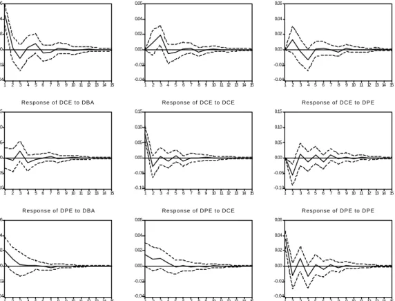
GRAPHIC 2

IMPULSE RESPONSE FUNCTION FOR CEARÁ, BAHIA AND PERNAMBUCO

-0.04 -0.02 0.00 0.02 0.04 0.06 1 2 3 4 5 6 7 8 9 10 11 12 13 14 15 R e s p o n s e o f D B A t o D B A -0.04 -0.02 0.00 0.02 0.04 0.06 1 2 3 4 5 6 7 8 9 10 11 12 13 14 15

Response of DBA to DCE

-0.04 -0.02 0.00 0.02 0.04 0.06 1 2 3 4 5 6 7 8 9 10 11 12 13 14 15 R e s p o n s e o f D B A t o D P E -0.10 -0.05 0.00 0.05 0.10 0.15 1 2 3 4 5 6 7 8 9 10 11 12 13 14 15

Response of DCE to DBA

-0.10 -0.05 0.00 0.05 0.10 0.15 1 2 3 4 5 6 7 8 9 10 11 12 13 14 15

Response of DCE to DCE

-0.10 -0.05 0.00 0.05 0.10 0.15 1 2 3 4 5 6 7 8 9 10 11 12 13 14 15

Response of DCE to DPE

-0.04 -0.02 0.00 0.02 0.04 0.06 1 2 3 4 5 6 7 8 9 10 11 12 13 14 15 R e s p o n s e o f D P E t o D B A -0.04 -0.02 0.00 0.02 0.04 0.06 1 2 3 4 5 6 7 8 9 10 11 12 13 14 15

Response of DPE to DCE

-0.04 -0.02 0.00 0.02 0.04 0.06 1 2 3 4 5 6 7 8 9 10 11 12 13 14 15 R e s p o n s e o f D P E t o D P E

Response to One S.D. Innovations ± 2 S.E.

through the estimation of impulse response functions from the VAR system of equations. GRAPHIC 2 shows the effects that a shock, equivalent to one standard deviation of the series, in one specific economy has in its own and in the other economies.

A shock in the economy of Bahia is very rapidly absorbed in the state. By the second year ,the shock is introduced and the positive effect in the economy disappear. The initial response of the Ceará economy to this shock is negative. Only after three years, it has some positive impact on it. The response of Pernambuco economy is positive but declining in the first three years.

A shock in the economy of Ceará appear to have positive and increasing effects on the economy of Bahia in the first three years after it takes place. After the fourth year, there are some negative effects. They do not, however, eliminate the cumulative positive effects observed early. The effect of the shock in the Pernambuco economy is firstly positive but it decreases rapidly in the following years. That is, in Bahia the initial effects are small but tend to increase over the following years, while in Pernambuco the initial effects are large but tend to decrease thereafter. The effects on Bahia of a Shock in the economy of Pernambuco are positive in the first two years but negative in the following three. The cumulated effect is close to zero. The economy of Ceará appears to be negatively effected by a shock in Pernambuco’s economy.

4 - CONCLUSION

In this paper we attempt to have a broad view on the interaction of the economies of the three largest states of Brazil’s Northeast. The empirical analysis is based on a VAR model of the states GSP.

The economies of Bahia and Pernambuco and of Ceará and Pernambuco appear to have contemporaneous economic cycles. The magnitudes of such comovements are not large, however. The economies of Ceará and Bahia do not appear to have any contemporaneous economic cycles.

The results indicate that past movement in the economy of Ceará tend to have initially small but increasing effects in the economy of Bahia, and large but decreasing effects on the economy of Pernambuco. On the other hand, a shock in the economy of Pernambuco appears to have little net effect on the economy of Bahia, but appears to hurt the economy of Ceará. That is, while the economies of Ceará and Bahia appear to be complementary the economies of Ceará and Perna mbuco appear to be competitors.

As an agenda for future researches, we can mention the estimation of structural reduced form specifications for the GSP of each state, and a close analysis of Input-output matrix available for the region. The main idea is to have a clearer picture of the process of economic development of the region. This will be achieved through a better understanding of the ways by which the states’ GSP are influenced by macroeconomic variables such as investment, interest rate, population, exports, etc, and the ways the region’s economic sectors interact to each other.

Resumo:

Parte da constatação de que o debate relativo ao desenvolvimento regional do Nordeste brasileiro tem se concentrado nos efeitos que políticas nacionais teriam na região. Pouca atenção tem sido dada a análise dos efeitos que a economia de um Estado específico pode trazer a outros Estados da região. Realiza um estudo empírico acerca da interação econômica entre os três maiores Estados da região Nordeste: Bahia, Ceará e Pernambuco. Faz a análise empírica baseada na estimação de um modelo VAR (Vector Autoregression Model) para os respectivos PIBs estaduais. As informações relativas à maneira pela qual as economia s interagem entre si são obtidas a partir da matriz de correlação dos resíduos do modelo VAR, de testes de causalidade de Granger e análise das funções de resposta de impulso derivados do respectivo modelo.

Palavras-chave:

Políticas Nacionais; Desenvolvimento Regional; Interação Econômica; Brasil-Nordeste.

5 - BIBLIOGRAFIA CONSULTADA

BOLETIM CONJUNTURAL. Nordeste do Bra-sil. SUDENE, nov. 1997. Fascículo.

CARLINO, G, DEFINA, R. Regional income

dynamics. Philadelphia: Federal Reserve Bank of Philadelphia , 1993. (Working Pa-per).

ENDERS, W. Applied econometric time series.

New York: John Wiley, 1995

ENGLE, R. F., Granger, C. W. J. Co-integration and error-correction: representation,

estima-tion, and testing. Econometrica, v. 55, p.

251-76, 1987

HAMILTON, J. D. Time series analysis.

Prince-ton:. Princeton University Press, 1994. LESAGE, P. J., PAN, Z. Using spatial contiguity as Bayesian prior information in regional

forecasting models. International Regional

Science Review, v. 18, p. 33-53, 1995

LUTKEPOHL, H. Differencing multiple time series: another look at Canadian money and

income data. Journal of Time Series

analy-sis, v. 3, p. 235-43, 1982

SIMS, C.A. Are forecasting models usable for

policy analysis? Quarterly Review of

Fede-ral Reserve Bank of Minne apolis,p. 2-16, winter 1986

_________. A comparison of interwar and post-war business cycles: monetarism

reconside-red. American Economic Review Papers

and Proceedings, v. 70, p. 250-257, 1980a

_________. Macroeconomics and reality.

Eco-nometrica, v.48, p. 1-48, 1980 b.

_________. Money, income, and causality.

Ame-rican Economic Review, v. 62, p. 540-553, 1972

_________. Policy analysis with econometrics

models. Brookings Papers of Economic

Activity, v. 2, p. 107-52, 1982. ________________