Modeling and Forecasting Implied Volatility an Econometric Analysis of the VIX Index

(1)

öMmföäflsäafaäsflassflassflas

ffffffffffffffffffffffffffffffffffff

Discussion Papers

Modeling and Forecasting Implied Volatility –

an Econometric Analysis of the VIX Index

Katja Ahoniemi

Helsinki School of Economics, FDPE, and HECER

Discussion Paper No. 129

October 2006

ISSN 1795-0562

HECER – Helsinki Center of Economic Research, P.O. Box 17 (Arkadiankatu 7), FI-00014

University of Helsinki, FINLAND, Tel +358-9-191-28780, Fax +358-9-191-28781,

(2)

HECER

Discussion Paper No. 129

Modeling and Forecasting Implied Volatility – an

Econometric Analysis of the VIX Index*

Abstract

This paper models the implied volatility of the S&P 500 index, with the aim of producing

useful forecasts for option traders. Numerous time-series models of the VIX index are

estimated, and daily out-of-sample forecasts are calculated from all relevant models. The

directional accuracy of the forecasts is evaluated with market-timing tests. Option trades

are simulated based on the forecasts, and their profitability is also used to rank the

models. The results indicate that an ARIMA(1,1,1) model enhanced with exogenous

regressors has predictive power regarding the directional change in the VIX index.

GARCH terms are statistically significant, but do not improve forecasts. The best models

predict the direction of change correctly for over 60 percent of the trading days.

Out-of-sample option trading over a period of fifteen months yields positive returns when the

forecasts from the best models are used as the basis for investment decisions.

JEL Classification

: C32, C53, G13

Keywords

: Implied volatility, Forecasting, Option markets

Katja Ahoniemi

Department of Economics,

Helsinki School of Economics

P.O. Box 1210

00101 Helsinki

FINLAND

e-mail:

katja.ahoniemi@hse.fi

*The author wishes to thank Markku Lanne, Pekka Ilmakunnas, and Petri Jylhä for

valuable comments. Financial support from the FDPE, the Jenny and Antti Wihuri

Foundation, the Okobank Group Research Foundation, the Finnish Foundation for Share

Promotion, and the Finnish Foundation for Advancement of Securities Markets is gratefully

acknowledged. This paper has been presented at the European Financial Management

Association 2006 Annual Meetings, Madrid, Spain, and at the 2006 Econometric Society

European Meetings, Vienna, Austria.

(3)

1

Introduction

Professional option traders such as hedge funds and banks’ proprietary traders are inter-ested primarily in the volatility implied by an option’s market price when making buy and sell decisions. If the implied volatility (IV) is assessed to be too high, the option is considered to be overpriced, and vice versa. Returns from volatility positions in op-tions, such as straddles, depend largely on the movements in IV, and the trader does not necessarily need a directional view regarding the price of the option’s underlying asset. The forecast accuracy of IV has been researched extensively, i.e. how well IV fore-casts the realized volatility over the life of an option. Christensen and Prabhala (1998) find that the volatility implied by S&P 100 index options predicts the actual volatility in the underlying index, but the forecasts are biased. Blair et al. (2001) find that volatil-ity forecasts provided by the VIX index are unbiased, and they outperform forecasts augmented with GARCH effects and high-frequency observations. Similar results were reported early on by Chiras and Manaster (1978) for individual stock options as well as by Jorion (1995) for foreign exchange options. In summary, most prevailing studies find that IV is most likely the best, although perhaps a biased, predictor of future realized volatility.

A clearly contradictory result comes from Canina and Figlewski (1993), who conclude that the IV of S&P 100 options has virtually no correlation with the future realized volatility. Day and Lewis (1992), who analyze S&P 100 index options, and Lamoureux and Lastrapes (1993), who study stock options, find that IV is biased and inefficient, as historical volatility can improve forecasts based on IV alone.

Relatively little work has been done on modeling IV, compared with the extensive literature on volatility modeling that exists today. Brooks and Oozeer (2002) and Har-vey and Whaley (1992) use regression models to forecast implied volatility and trade accordingly. Both studies suggest profits for a market maker, but not for a trader fac-ing transaction costs. Mixon (2002) uses regression models to find that domestic stock returns explain changes in IV well.

Also, few studies explore option trading in connection with IV analysis, and those studies that do simulate trades employ strategies that are not favored among actual mar-ket participants. Harvey and Whaley (1992), Brooks and Oozeer (2002) and Corredor et al. (2002) employ simple buy or sell option trading strategies, whereas typical option trades involve various types of spreads, such as the straddle. Noh et al. (1994) simulate straddle trades, and in the trading simulation of Poon and Pope (2000), S&P 100 call options are bought and S&P 500 call options simultaneously sold, or vice versa. Coval and Shumway (2001) focus on pure option trading, calculating returns for long call, long put, and long straddle positions, with no time series analysis or other decision rule in the background.

The objective of this study is to model and forecast implied volatility, with the ultimate aim of producing relevant information for option traders. The goal of the model-building is to find a model that would reliably forecast the future direction of IV, thus providing valuable signals to option traders. The success of the forecasts will be evaluated with their directional accuracy, with a market timing test, and by simulating option trades with true market prices and calculating the profitability of the trades.

An ARIMA(1,1,1) model augmented with the returns of the S&P 500 index and the returns of the MSCI EAFE index is found to be a good fit for a time series of the VIX index. This model specification produces forecasts with a directional accuracy of up

(4)

to 62 percent. Option trades simulated on the basis of these forecasts lead to positive returns in a fifteen-month out-of-sample period.

This paper proceeds as follows. Section 2 describes the data used in this study, Section 3 presents the models estimated for the VIX time series, Section 4 contains the analysis of forecasts, and Section 5 discusses the option trading simulations. Section 6 concludes.

2

Data

2.1 Implied volatility

Implied volatility is calculated by solving an option pricing model for the volatility when the prevailing market price for an option is known. Volatility is the only ambiguous input into e.g. the Black-Scholes option pricing formula, which is shown below for a call option: C =SN(d1)−Xe−rTN(d2) (1) where d1 = ln(S/X)+(r+σ 2_/₂₎_T σ√T d2=d1−σ √ T

C denotes the price of a European call option,S is the market price of the underlying asset, X is the strike price of the option,r is the risk-free interest rate, T is the time to maturity of the option, N is the cumulative normal distribution function, and σ is the volatility in the returns of the underlying asset during the life of the option.

The Black-Scholes pricing model makes two assumptions that are in contrast with what is observed in actual financial markets. First, the model assumes that the volatility in the price of the underlying asset will remain constant throughout the life of the option. Second, the logarithmic returns of the underlying asset are assumed to follow a normal distribution, whereas financial market returns exhibit both skewness and excess kurtosis. The non-normality of financial returns is manifested in the fact that when IVs are calculated from prevailing market prices with the Black-Scholes model, the so-called volatility smile or volatility skew emerges: IVs vary with the strike price of options, even for options with the same maturity date.

2.2 The VIX index

The core data in this study consists of daily observations of the VIX volatility index calculated by the Chicago Board Options Exchange1_{. The VIX, introduced in 1993, is}

derived from the bid/ask quotes of options on the S&P 500 index. It is widely followed by financial market participants and is considered not only to be the market’s expectation of the volatility in the S&P 500 index over the next month, but also to reflect investor sentiment and risk aversion. If investors grow more wary, the demand for above all put

(5)

options will rise, thus increasing IV and the value of the VIX. Also, e.g. Blair et al. (2001) and Mayhew and Stivers (2003) use the VIX as an indicator of market implied volatility.

The calculation method of the VIX was changed on September 22, 2003 to bring it closer to actual financial industry practises. From that day onwards, the VIX has been based on S&P 500 rather than S&P 100 options: the S&P 500 index is the most commonly used benchmark for the U.S. equity market, and the most popular underlying for U.S. equity derivatives. A wider range of strike prices is included in the calculation, making the new VIX more robust. Also, the Black-Scholes formula is no longer used, but the methodology is independent of a pricing model. In practise, the VIX is calculated directly from option prices rather than solving it out of an option pricing formula. Values for the VIX with the new methodology are available from the CBOE from 2.1.1990. The data set used in this study consists of daily observations covering fifteen years, from 2.1.1990 to 31.12.2004. Public holidays that fall on weekdays, when the CBOE is closed, were omitted from the data set.

The VIX is calculated using the two nearest expiration months of S&P 500 options in order to achieve a 30-calendar-day period2. Rollover to the next expiration occurs eight calendar days prior to the expiry of the nearby option. The value of the index is derived from the prices of at-the-money and out-of-the-money calls and puts. The closer the option’s strike price to the at-the-money value, the higher the weight its price receives in the calculation. The formula for calculating the VIX index is:

σ2 = 2 T X i ∆K_i K2 i erTQ(Ki)− 1 T " F K0 −1 #₂ (2)

whereσis the value of the VIX divided by 100, T is the time to expiration of the option contract,F is the forward index level derived from option prices,Ki is the strike price of

theith _{out-of-the-money option (call if}_K

t> F and put ifKt< F), ∆Ki is the interval

between strike prices, or (Ki+1−Ki−1)/2,K0is the first strike belowF,ris the risk-free

interest rate up to the expiration of the option contract, andQ(Ki) is the midpoint of

the bid-ask spread for each option with strikeK_i. Calls and puts are included up to the point where there are two consecutive strike prices with a bid price equal to zero.

The use of the VIX index considerably alleviates the problems of measurement errors and model misspecification. The simultaneous measurement of all variables required by an option pricing model is often difficult to achieve. When the underlying asset of an option is a stock index, infrequent trading in one of the component stocks of the index can lead to misvaluation of the index level. Also, there is no correct measure for the volatility required as an input in a pricing model such as Black-Scholes. The chosen option pricing model for IV calculation is critical, as the assumptions of the model can greatly affect the resulting value for IV. If a European option valuation model is used to determine the IV of an American option, an erroneous value will result.

(6)

2.3 Other data

Data on various financial and macroeconomic indicators was also obtained from the Bloomberg Professional service to test whether they could help explain the variations in the VIX. The data set contains the S&P 500 index, the trading volume of the S&P 500 index, the MSCI EAFE (Europe, Australasia, Far East) index, the three-month USD LIBOR interest rate, the 10-year U.S. government bond yield, and the price of crude oil from the next expiring futures contract. Data on the S&P 500 trading volume is available only from 4.1.1993 onwards.

The out-of-sample performance of option trades executed based on the analysis of the VIX time series will be tested with the daily open and close quotes of near-the-money S&P 500 index options, which are quoted on the Chicago Board Options Exchange. The options in the data set were selected on a monthly basis so that all options that were at-the-money at least momentarily during the month in question were included as possibilities. Only the two nearest expirations are considered, as they are overwhelm-ingly the most liquid3_{. The S&P 500 option quotes were obtained from the Bloomberg}

Professional service for the 15-month period of 1.10.2003 to 31.12.2004.

3

Modeling the VIX

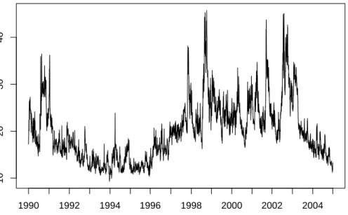
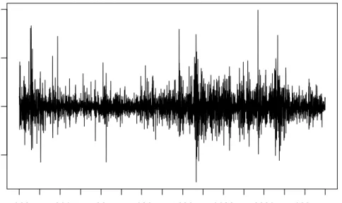
The VIX index was relatively stable in the early 1990s, but more volatile from the last quarter of 1997 to the first quarter of 2003. Figure 1 shows the daily level of the VIX for the entire sample. Clear spikes in the value of the VIX coincide with the Asian financial crisis of late 1997, the Russian and LTCM crisis of late 1998, and the 9/11 terrorist attacks. A visual inspection of the VIX first differences points to heteroskedasticity in the data, as can be seen in Figure 2.

10

20

30

40

1990 1992 1994 1996 1998 2000 2002 2004

Figure 1: VIX index 1.1.1990 - 31.12.2004

3_{Poon and Pope (2000) analyze S&P 100 and S&P 500 option trading data for a period of 1,160}

trading days and find that contracts with 5-30 days of maturity have the highest number of transactions and largest trading volume. At-the-money and slightly out-of-the-money options are most heavily traded.

(7)

−5

0

5

10

1990 1992 1994 1996 1998 2000 2002 2004

Figure 2: VIX first differences 1.1.1990 - 31.12.2004

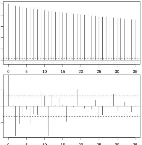
Logarithms of the VIX observations were taken in order to avoid negative forecasts of volatility. The daily logarithmic levels of VIX display high autocorrelation, as shown in Figure 3. The autocorrelations for the differenced time series are also shown in Figure 3.

A unit root is rejected by the augmented Dickey-Fuller (ADF) test for both the level (p-value 0.0006) and differenced (p-value 0.0000) time series at the one-percent level of significance. The lag lengths in the ADF tests are four for the level series and ten for the differenced series, based on selection with the Bayesian Information Criterion.

ARM A and ARF IM A models were estimated for the VIX levels, but despite the high persistence in the time series, even the ARF IM Amodels failed to produce useful forecasts (directional accuracy of over 50 percent). Also, the value received fordin the

ARF IM Amodeling exceeded 0.49 when its value was restricted to be less than 0.5, and fell within the non-stationary range of [0.5,1] when no restrictions were placed on its value. In light of this evidence, the models in this study were built for log VIX first differences rather than levels.

Descriptive statistics for the VIX first differences are provided in Table 1. The VIX is skewed to the right, and it displays excess kurtosis.

Full sample In-sample

Maximum 0.416861 0.416861 Minimum -0.275054 -0.275054 Mean -0.000069 0.000155 Median -0.002547 -0.001691 Standard deviation 0.055931 0.057527 Skewness 0.595536 0.607743 Excess kurtosis 3.62725 3.63307

Table 1: Descriptive statistics for VIX first differences. Full sample: 1.1.1990-31.12.2004, in-sample: 1.1.1990-31.12.2002.

(8)

0 5 10 15 20 25 30 35 0.0 0.2 0.4 0.6 0.8 1.0 0 5 10 15 20 25 30 35 −0.05 0.00 0.05

(9)

robustness of the results and stability of coefficients over time. The time periods are listed in Table 2. Period 1 covers the entire in-sample. The dates chosen for Period 2 reflect the starting point of more volatile behavior in the VIX. Periods 3 and 4 were chosen based on the number of observations. Studies such as Noh et al. (1994) and Blair et al. (2001) use 1,000 observations when calculating forecasts fromGARCH models. Forecasts were also calculated with only 500 observations to see whether forecast performance would improve with only a short period of observations: conditions in financial markets can change rapidly, and perhaps only the most recent information is relevant for forecasting purposes. The in-sample estimation period ends for all time periods on 31.12.2002, and the first forecasts are calculated for 2.1.2003.

Period Dates No. of observations

Period 1 1.1.1990-31.12.2002 3260

Period 2 1.10.1997-31.12.2002 1314

Period 3 4.1.1999-31.12.2002 1000

Period 4 29.12.2000-31.12.2002 500

Table 2: Time periods in coefficient estimation

3.1 Linear models

Based on tests for autocorrelation and the p-values of the coefficients, anARIM A(1,1,1) specification was found to be the best fit for the log VIX time series from the family of

ARM Amodels. TheARIM A(1,1,1) model was then augmented withGARCH errors and exogenous regressors. Goodness-of-fit was compared primarily with the Bayesian Information Criterion (BIC), and secondly with the coefficient of determination R2_.

Heteroskedasticity-robust standard errors were used throughout the analysis. In all

esti-mation withGARCH errors, the estimation method was Gaussian maximum likelihood.

A number of macroeconomic indicators were included in the regressions to see whether they could improveARIM Amodels of the VIX. These variables were the returns in the S&P 500 index, the one-month, or 22-trading-day, historical volatility of the S&P 500 index and its first difference, the spread between the VIX and the historical volatility of the S&P 500 index and its first difference, the trading volume of the S&P 500 index and its first difference, the returns of the MSCI EAFE (Europe, Australasia, Far East) index, the first difference of the three-month USD LIBOR interest rate, the first difference of the slope of the yield curve proxied by the 10-year rate less the 3-month rate, and the first difference of the price of oil from the next expiring futures contract. Many variables similar to these have been used by e.g. Franks and Schwartz (1991).

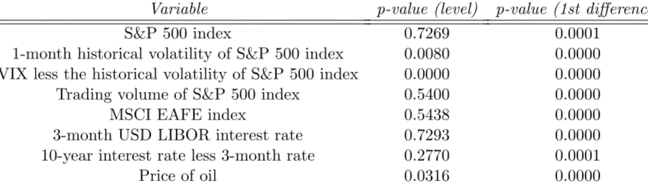
Logarithms were used for all variables except the slope of the yield curve. Use of the S&P 500 trading volume, the short-term interest rate, and the slope of the yield curve without differencing was ruled out by the ADF test (see Table 3). The p-values from the ADF test indicate that the null hypothesis of a unit root cannot be rejected at the one-percent level for the above-mentioned time series. Also, returns must naturally be used for the S&P 500 and MSCI EAFE index returns. The returns of the S&P 500 index, its trading volume, and returns in the MSCI EAFE index in particular could be assumed to have some effect on changes in the VIX. High trading volume could be a signal of e.g. panic selling, linked to rising IV.

(10)

Positive and negative returns in the S&P 500 index were separated by forming sep-arate variables for each, as negative shocks have a tendency of raising volatility more than positive shocks. Dividend payouts are not taken into account in calculating the returns of the S&P 500 index.

Variable p-value (level) p-value (1st difference)

S&P 500 index 0.7269 0.0001

1-month historical volatility of S&P 500 index 0.0080 0.0000

VIX less the historical volatility of S&P 500 index 0.0000 0.0000

Trading volume of S&P 500 index 0.5400 0.0000

MSCI EAFE index 0.5438 0.0000

3-month USD LIBOR interest rate 0.7293 0.0000

10-year interest rate less 3-month rate 0.2770 0.0001

Price of oil 0.0316 0.0000

Table 3: P-values from ADF tests for a unit root in explanatory variables.

The six linear models that were estimated for the differenced VIX time series are listed in Table 4. The regression results indicate that an ARIM A(1,1,1) model is the best ARIM A specification. The exogenous regressors that were found to improve the fit of the model and have statistically significant coefficients were the returns of the MSCI EAFE index as well as the positive and negative returns of the S&P 500 index. Data on the S&P 500 index trading volume was available for all time periods except Period 1. Its first differences were added to the analysis (Models 5 and 6) in order to check for possible improvements to forecasts, although its coefficient was not statistically significant. The addition of aGARCH specification fits the chosen models, with

statis-tically significant coefficients for both theARCH andGARCH terms. GARCH models

were only estimated with a minimum of 1,000 observations, as estimates of conditional heteroskedasticity may be unreliable with a small sample size4_.

Linear models

Model ARIMA / GARCH Exogenous regressors

Model 1 ARIMA(1,1,1)

-Model 2 ARIMA(1,1,1) + GARCH(1,1)

-Model 3 ARIMA(1,1,1) W P N

Model 4 ARIMA(1,1,1) + GARCH(1,1) W P N

Model 5 ARIMA(1,1,1) W P N V

Model 6 ARIMA(1,1,1) + GARCH(1,1) W P N V

Table 4: Linear models. W=log returns of the MSCI EAFE index, P=positive log returns of the S&P 500 index, N=negative log returns of the S&P 500 index, V=first differences of log S&P 500 trading volume.

In practise, the estimated linear equation is:

V IXRt=c+β1V IXRt−1+β2²t−1+β3Wt+β4Pt−1+β5Nt−1+β6Vt−1+²t (3) 4_{This is the minimum number of observations used by e.g. Blair et al. (2001) and Noh et al. (1994)}

when calculating volatility forecasts from GARCH models. Engle et al. (1993) calculate variance forecasts for an equity portfolio and find thatARCH models using 1,000 observations perform better than models with 300 or 5,000 observations.

(11)

where V IXR=first differences of the logarithms of the VIX index, W=log returns of the MSCI EAFE index, P=positive log returns of the S&P 500 index, N=negative log returns of the S&P 500 index, V=log first differences of S&P 500 trading volume. As in the models of e.g. Davidson et al. (2001) and Simon (2003),P is equal to the return of the S&P 500 index when the return is positive, and zero otherwise. Likewise forN, it is equal to the return of the S&P 500 index when the return is negative, and zero otherwise. The time indexing ofW differs from the other variables, as its value is known to traders in the U.S. markets before the local market opens for trading: W is calculated from the returns of Asian and European markets. Therefore,Wtcan be used to explain

V IXRt, and information that is as up-to-date as possible is utilized.

In Models 2, 4, and 6, GARCH(1,1) errors with a Gaussian distribution are used.

GARCH models are based on the autoregressive conditional heteroskedasticity model introduced by Engle (1982) and generalized by Bollerslev (1986). In theGARCH(1,1) model,²is defined as:

²t=zth1t/2

wherezt is a sequence ofi.i.d.∼(0,1) random variables and

h_t=α₀+α₁²2

t−1+β1ht−1

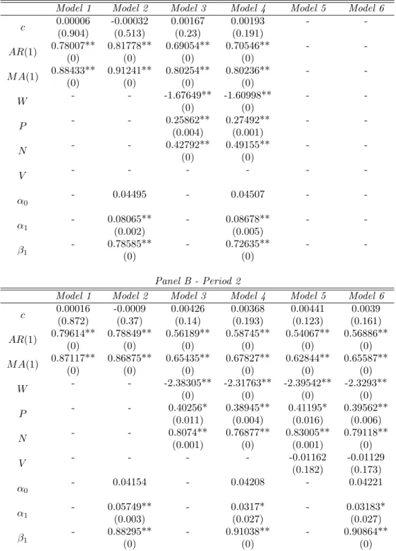
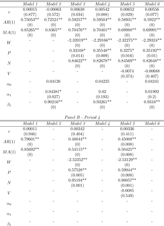
The coefficients and their p-values for all six models are presented in Table 5 for Periods 1 and 2 and in Table 6 for Periods 3 and 4. The AR(1) and M A(1) terms are statistically significant at the one-percent level throughout, and the returns of the MSCI EAFE index and the S&P 500 index are significant at the five-percent level.

The changes in S&P 500 trading volume are not statistically significant, but the possible improvementV will provide to forecasts will be evaluated in Section 4. GARCH

terms are significant at the five-percent level throughout, with the exception of Models

4 and 6 in Period 3, or when the number of observations in GARCH estimation is

smallest. The coefficients in the models evolve over time, as was to be expected based on the visual analysis of the VIX time series. In Period 4, with only 500 observations, the impacts of MSCI EAFE and S&P 500 returns are largest.

The coefficients of N are larger in absolute value than the coefficients of P for all the linear models. In other words, negative returns impact the VIX more than positive returns, which is consistent with earlier findings about the larger effect of negative shocks in financial markets. This finding has been reported by e.g. Fleming et al. (1995) for the VIX index and by Simon (2003) for the VXN, or the Nasdaq 100 Volatility Index. They estimated negative coefficients for contemporaneous positive and negative returns in the underlying index. Thus, positive contemporaneous returns lower the VIX, but negative contemporaneous returns raise IV and thus the index level.

In this study, S&P 500 index returns are not contemporaneous, but lagged. The option trader opens her positions at the start of the day, without knowing how the stock market will develop during the day. Therefore, the best available information comes from dayT−1. The positive coefficients in this study can be interpreted as a reflection of mean reversion: a positive S&P 500 return may have lowered the VIX during dayT, so in day T + 1, the VIX rises. Similarly for negative returns, a rise in the VIX in day

T is followed by a fall in day T+ 1. On the other hand, the negative coefficient for the MSCI EAFE index is in line with the results of Fleming et al. (1995) and Simon (2003). The foreign stock market return is contemporaneous, so a negative coefficient leads to

(12)

a drop in the VIX if the return in foreign markets has been positive, and vice versa for negative foreign market returns.

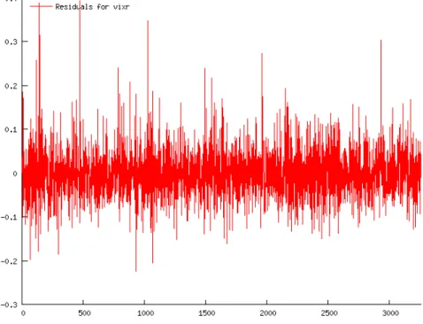
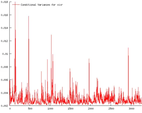
The residuals for Model 3 in Period 1 are shown in Figure 4 and the conditional vari-ances for Model 4 in Period 1 are shown in Figure 5. The clustering in the residuals and the spikes in the conditional variances again point to the conditional heteroskedasticity in the time series of VIX first differences. These figures are provided as representa-tive examples, and the equivalent figures from other pairs of models with and without

GARCH errors are similar.

Figure 4: Residuals for Model 3, period 1

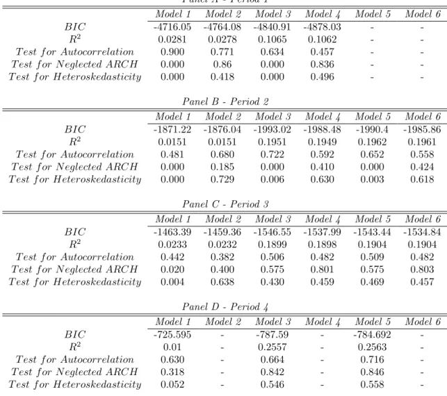
Goodness-of-fit measures and test statistics are given in Table 7. The BIC and R2

measures reveal that the goodness-of-fit of the models improves clearly with the addition of exogenous regressors. However, the addition ofV to the set of regressors (Models 5 and 6) no longer improves the goodness-of-fit. Based on the BIC, Model 3 is the best specification in all periods except Period 1, where it is outperformed by Model 4.

GARCH errors make a pronounced change to the test results for the models in Peri-ods 1 and 2. After addingGARCH errors to the models, the null hypotheses of tests for neglected ARCH and heteroskedasticity are rejected at the five-percent level. Accord-ing to the tests, Models 3 and 5 are free of neglectedARCH and heteroskedasticity in Periods 3 and 4, but this may be due to weaker power of the tests with a small number of observations used in the estimation. The Breusch-Godfrey test for autocorrelation indicates that the null hypothesis of no autocorrelation cannot be rejected for any of the considered models in any of the time periods.

3.2 Probit models

As the focus in this study is on obtaining the correct direction of change in the VIX index (up or down) rather than the correct magnitude, binary probit models were also

(13)

Panel A - Period 1

Model 1 Model 2 Model 3 Model 4 Model 5 Model 6

c 0.00006 -0.00032 0.00167 0.00193 - -(0.904) (0.513) (0.23) (0.191) AR(1) 0.78007** 0.81778** 0.69054** 0.70546** - -(0) (0) (0) (0) M A(1) 0.88433** 0.91241** 0.80254** 0.80236** - -(0) (0) (0) (0) W - - -1.67649** -1.60998** - -(0) (0) P - - 0.25862** 0.27492** - -(0.004) (0.001) N - - 0.42792** 0.49155** - -(0) (0) V - - - -α0 - 0.04495 - 0.04507 - -α1 - 0.08065**_(0.002) - 0.08678**_(0.005) - -β1 - 0.78585**₍₀₎ - 0.72635**₍₀₎ - -Panel B - Period 2

c 0.00016 -0.0009 0.00426 0.00368 0.00441 0.0039 (0.872) (0.37) (0.14) (0.193) (0.123) (0.161) AR(1) 0.79614** 0.78849** 0.56189** 0.58745** 0.54067** 0.56886** (0) (0) (0) (0) (0) (0) M A(1) 0.87117** 0.86875** 0.65435** 0.67827** 0.62844** 0.65587** (0) (0) (0) (0) (0) (0) W - - -2.38305** -2.31763** -2.39542** -2.3293** (0) (0) (0) (0) P - - 0.40256* 0.38945** 0.41195* 0.39562** (0.011) (0.004) (0.016) (0.006) N - - 0.8074** 0.76877** 0.83005** 0.79118** (0.001) (0) (0.001) (0) V - - - - -0.01162 -0.01129 (0.182) (0.173) α0 - 0.04154 - 0.04208 - 0.04221 α1 - 0.05749**_(0.003) - 0.0317*_(0.027) - 0.03183*_(0.027) β1 - 0.88295**₍₀₎ - 0.91038**₍₀₎ - 0.90864**₍₀₎

Table 5: Coefficients from linear model estimation (Periods 1 and 2). P-values in parentheses. (**) denotes statistical significance at the 1% level, and (*) at the 5% level.

(14)

c 0.00015 -0.00063 0.00638 0.00542 0.00652 0.00556 (0.877) (0.572) (0.034) (0.088) (0.029) (0.077) AR(1) 0.75053** 0.72521** 0.59257** 0.59504** 0.58931** 0.5922** (0) (0) (0) (0) (0) (0) M A(1) 0.85265** 0.8365** 0.70476** 0.70401** 0.69988** 0.69991** (0) (0) (0) (0) (0) (0) W - - -2.32019** -2.29166** -2.32275** -2.29324** (0) (0) (0) (0) P - - 0.33108* 0.35548** 0.3275* 0.35192** (0.014) (0.009) (0.016) (0.01) N - - 0.84622** 0.82678** 0.84569** 0.82648** (0) (0) (0) (0) V - - - - -0.0074 -0.00688 (0.374) (0.407) α0 - 0.04126 - 0.04225 - 0.04241 α1 - 0.04381*_(0.027) - _(0.193)0.02 - 0.01992_(0.2) β1 - 0.90216**₍₀₎ - 0.93261**₍₀₎ - 0.9316**₍₀₎ Panel B - Period 4

c 0.00011 - 0.00342 - 0.00336 -(0.946) (0.404) (0.411) AR(1) 0.79601** - 0.48044** - 0.45008** -(0) (0) (0.008) M A(1) 0.85692** - 0.54115** - 0.50425** -(0) (0) (0.008) W - - -2.52352** - -2.53129** -(0) (0) P - - 0.57528** - 0.59944** -(0.005) (0.008) N - - 0.95194** - 0.98057** -(0.001) (0.001) V - - - - -0.0085 -(0.549) α0 - - - -α1 - - - -β1 - - -

-Table 6: Coefficients from linear model estimation (Periods 3 and 4). P-values in parentheses. (**) denotes statistical significance at the 1% level, and (*) at the 5% level.

(15)

BIC -4716.05 -4764.08 -4840.91 -4878.03 -

-R2 _0.0281 _0.0278 _0.1065 _0.1062 _-

-T est f or Autocorrelation 0.900 0.771 0.634 0.457 -

-T est f or N eglected ARCH 0.000 0.86 0.000 0.836 -

-T est f or Heteroskedasticity 0.000 0.418 0.000 0.496 -

-Panel B - Period 2

BIC -1871.22 -1876.04 -1993.02 -1988.48 -1990.4 -1985.86

R2 _0.0151 _0.0151 _0.1951 _0.1949 _0.1962 _0.1961

T est f or Autocorrelation 0.481 0.680 0.722 0.592 0.652 0.558

T est f or N eglected ARCH 0.000 0.185 0.000 0.410 0.000 0.424

T est f or Heteroskedasticity 0.000 0.729 0.006 0.630 0.003 0.618

Panel C - Period 3

BIC -1463.39 -1459.36 -1546.55 -1537.99 -1543.44 -1534.84

R2 _0.0233 _0.0232 _0.1899 _0.1898 _0.1904 _0.1904

T est f or Autocorrelation 0.442 0.382 0.506 0.482 0.509 0.482

T est f or N eglected ARCH 0.020 0.400 0.575 0.801 0.575 0.803

T est f or Heteroskedasticity 0.004 0.638 0.430 0.459 0.469 0.457

Panel D - Period 4

BIC -725.595 - -787.59 - -784.692

-R2 _0.01 _- _0.2557 _- _0.2563

-T est f or Autocorrelation 0.630 - 0.664 - 0.716

-T est f or N eglected ARCH 0.318 - 0.842 - 0.846

-T est f or Heteroskedasticity 0.052 - 0.546 - 0.558

-Table 7: Statistics and tests for linear models. The tests are Lagrange multiplier tests, with p-values provided. Five lags are used in the tests for autocorrelation and neglectedARCH. The test for autocorrelation is the Breusch-Godfrey LM test statistic. The test for neglectedARCH is Engle’s LM test statistic, computed from a regression of squared residuals on lagged squared residuals. The test for heteroskedasticity is computed from a regression of squared residuals on squared fitted values. The asymptotic distribution of all the test statistics isχ2_.

(16)

Figure 5: Conditional variances for Model 4, period 1

estimated. This will enable a check of whether the linear models, which are estimated with more precise information, provide added value to the forecasts, even though the focus is on the direction of change. With probit models, a move upwards was marked 1 and a change downwards as 0:

yt=1[V IXRt>0], t= 1,2, ..., T

where 1[·] is an indicator function.

The same explanatory variables that were used in linear models were found to be significant in probit models as well. In addition, the lagged binary variable was also included as a regressor in two of the four models (see Table 8). The explanatory power of the lagged binary variable is not likely to be very good, however, as the VIX is a mean reverting time series. Models 3 and 4 were not estimated from Period 1, as data on the S&P 500 index trading volume is only available from the beginning of 1993.

Probit models

Model Lagged binary variable Exogenous regressors

Model 1 - W P N

Model 2 X W P N

Model 3 - W P N V

Model 4 X W P N V

Table 8: Probit models. W=log returns of the MSCI EAFE index, P=positive log returns of the S&P 500 index, N=negative log returns of the S&P 500 index, V=first differences of log S&P 500 trading volume.

(17)

p=F(Z) =

Z _Z

−∞

f(Z)dZ (4) whereF(·) is the cumulative standardized normal distribution. The equation forZ that is estimated in this study is given in Equation 5:

BINt+1 =c+β1Wt+1+β2Pt+β3Nt+β4Vt+β5BINt+²t+1 (5)

whereBIN is a binary variable that receives the value 1 when the VIX index rises, and the value 0 when the VIX index falls.

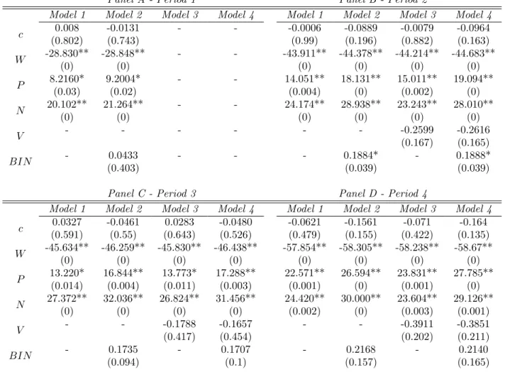
The coefficients from the probit estimation are given in Table 9. The lagged binary variables and V are not statistically significant, but W, P, and N are all significant at the five-percent level. Similar to the linear models, the impact of negative S&P 500 returns is larger than the impact of positive returns (with the exception of Model 3 in Period 4). The signs of the coefficients in the probit models are the same as the signs in the linear models.

Panel A - Period 1 Panel B - Period 2

Model 1 Model 2 Model 3 Model 4 Model 1 Model 2 Model 3 Model 4

c 0.008 -0.0131 - - -0.0006 -0.0889 -0.0079 -0.0964 (0.802) (0.743) (0.99) (0.196) (0.882) (0.163) W -28.830** -28.848** - - -43.911** -44.378** -44.214** -44.683** (0) (0) (0) (0) (0) (0) P 8.2160* 9.2004* - - 14.051** 18.131** 15.011** 19.094** (0.03) (0.02) (0.004) (0) (0.002) (0) N 20.102** 21.264** - - 24.174** 28.938** 23.243** 28.010** (0) (0) (0) (0) (0) (0) V - - - -0.2599 -0.2616 (0.167) (0.165) BIN - 0.0433 - - - 0.1884* - 0.1888* (0.403) (0.039) (0.039)

Panel C - Period 3 Panel D - Period 4

Model 1 Model 2 Model 3 Model 4 Model 1 Model 2 Model 3 Model 4

c 0.0327 -0.0461 0.0283 -0.0480 -0.0621 -0.1561 -0.071 -0.164 (0.591) (0.55) (0.643) (0.526) (0.479) (0.155) (0.422) (0.135) W -45.634** -46.259** -45.830** -46.438** -57.854** -58.305** -58.238** -58.67** (0) (0) (0) (0) (0) (0) (0) (0) P 13.220* 16.844** 13.773* 17.288** 22.571** 26.594** 23.831** 27.785** (0.014) (0.004) (0.011) (0.003) (0.001) (0) (0.001) (0) N 27.372** 32.036** 26.824** 31.456** 24.420** 30.000** 23.604** 29.126** (0) (0) (0) (0) (0.002) (0) (0.003) (0.001) V - - -0.1788 -0.1657 - - -0.3911 -0.3851 (0.417) (0.454) (0.202) (0.211) BIN - 0.1735 - 0.1707 - 0.2168 - 0.2140 (0.094) (0.1) (0.157) (0.165)

Table 9: Coefficients from probit estimation. P-values in parentheses. (**) denotes statistical signifi-cance at the 1% level, and (*) at the 5% level.

Measures of goodness-of-fit and p-values from tests for autocorrelation and het-eroskedasticity are provided in Table 10. The addition of the changes in S&P 500

(18)

trading volume does not improve the goodness-of-fit of the models, and neither does the inclusion of the lagged binary variable. The BIC indicates that Model 1 outperforms the other models in all periods. Coefficients of determination are clearly best for models estimated in Period 4, or with 500 observations.

The LM test for autocorrelation rejects the null hypothesis at the five-percent level for nine of the fourteen probit models. Heteroskedasticity is rejected at the five-percent level only for the models in Period 2. The rejections in Periods 3 and 4 may again be due to weaker power with smaller numbers of observations, however.

Model 1 Model 2 Model 3 Model 4

BIC 2204.08 2207.77 -

-R2 _0.042 _0.042 _-

-T est f or Autocorrelation 0.002 0.002 -

-T est f or Heteroskedasticity 0.052 0.078 -

-Panel B - Period 2

BIC 853.484 854.889 856.164 857.561

R2 _0.1012 _0.1041 _0.1028 _0.1057

T est f or Autocorrelation 0.022 0.073 0.032 0.091

T est f or Heteroskedasticity 0.005 0.008 0.010 0.020

Panel C - Period 3

BIC 653.111 655.172 656.249 658.356

R2 _0.1005 _0.1029 _0.1014 _0.1037

Panel D - Period 4

BIC 310.726 312.831 313.04 315.173

R2 _0.1744 _0.1785 _0.1782 _0.1821

Table 10: Statistics and tests for probit models. Five lags are used in the LM tests for autocorrelation and heteroskedasticity, whose p-values are provided. The R2 _{is the squared correlation between the}

predictions from the normal CDF and the binary actuals.

4

Forecasts

The next step in the analysis is to obtain forecasts from the models described in Section 3. Out-of-sample, one-step-ahead forecasts were calculated for the VIX first differences. In practise, the predicted direction of change was calculated on a daily basis.

Forecasts were calculated from all models presented above, estimated with numbers of observations equal to those used in the four time periods. Therefore, the first series of forecasts is estimated with 3,260 observations, the second series with 1,314 observations, the third series with 1,000 observations, and the fourth series with 500 observations.

(19)

The forecasts were calculated from rolling samples, keeping the sample size constant each day. In other words, after calculating each forecast, the furthest observations are dropped, the observations for the most recent day are added to the sample, and the model is re-estimated. For comparison, Model 3 was also estimated with an incremen-tal (growing) sample size starting with 3,260 and 1,314 observations, i.e. by adding the newest observations to the sample each day, but dropping no observations5_{. This}

introduces a seventh linear model into the analysis, Model 3I.

Once each model is estimated up to dayT, the values of the regressors for dayT are plugged in to obtain the forecast for the change in the VIX from day T to day T+ 1. Again, the only variable that is treated differently is the MSCI EAFE index, whose value forT+ 1 is used when calculating the forecasts.

Successful forecasting of IV from an option trader’s point of view involves forecasting the direction of IV correctly; a correct magnitude for the change is not as relevant. This is because positions such as the straddle will generate a profit if the IV moves in the correct direction, ceteris paribus (the size of the profit is affected by the magnitude of change, however). The forecasting accuracy of the various models is evaluated based on sign: how many times does the sign of the change in the VIX correspond to the direction forecasted by the model.

The first forecast is calculated for 2.1.2003, and the last for 31.12.2004. This amounts to 501 days of forecasts. Table 11 shows the forecast performance of the various models, measured with the correct direction of change. The linear and probit models succeed in predicting the direction of change correctly for 52-62 percent of the trading days. This performance is in line with the results of e.g. Pesaran and Timmermann (1995) and Gen¸cay (1998).

For linear models, the addition of exogenous regressors clearly improves the forecast

performance, but improvements from addingGARCH errors are negligible. The number

of observations used in the model estimation affects the accuracy of the sign predictions hardly at all. The best accuracy, or 310 correct signs out of 501 days, comes from both Model 6 with 1,000 observations and Model 3 with 500 observations. No clear conclusion can be drawn on whether or not it is beneficial to includeV as a regressor.

With probit models, the forecasts are probabilities that the outcome will be 1. All forecasts over 50 percent were interpreted as a move upwards, and forecasts below 50 percent were taken as a forecast of the value of the VIX falling. The best performer is Model 4 with 1,000 observations, which produces 299 correct directional forecasts. How-ever, the share of correct signs is close to equal for all the probit models. The addition of the lagged binary variable both improves and weakens the forecasting performance, depending on the model and number of observations. Thus, the number of observations and exact model specification from among the four alternatives seem to hold little rel-evance. It can be noted that all linear models, with the exception of Models 1 and 2, provide better forecasts than the best probit model.

In the spirit of the particular nature of this study, the predictive ability of the models was tested using the market timing test for predictive accuracy developed by Pesaran and Timmermann (1992). The Pesaran-Timmermann test (henceforth PT test) was originally developed with the idea that an investor switches between stocks and bonds depending on the returns expected from each asset class.

The PT test is calculated with the help of a contingency table (Table 12). The

5_{E.g. Lamoureux and Lastrapes (1993) use both rolling and incremental sample size in their variance}

(20)

Panel A -line ar 3260 observations 1314 observations 1000 observations 500 observations Corr. sign % MSE Corr. sign % MSE Corr. sign % MSE Corr. sign % MSE Mo del 1 271 54.1% 0.00196 270 53.9% 0.00192 266 53.1% 0.00193 263 52.5% 0.00192 Mo del 2 277 55.3% 0.00191 274 54.7% 0.00192 272 54.3% 0.00193 -Mo del 3 305 60.9% 0.00169 305 60.9% 0.00170 307 61.3% 0.00170 310 61.9% 0.00171 Mo del 4 308 61.5% 0.00169 304 60.7% 0.00169 309 61.7% 0.00170 -Mo del 5 -306 61.1% 0.00170 306 61.1% 0.00171 305 60.9% 0.00174 Mo del 6 -305 60.9% 0.00170 310 61.9% 0.0017 -Mo del 3I 309 61.7% 0.00169 305 60.9% 0.00170 -Panel B -pr obit 3260 observations 1314 observations 1000 observations 500 observations Corr. sign % MSE Corr. sign % MSE Corr. sign % MSE Corr. sign % MSE Mo del 1 293 58.5% -291 58.1% -290 57.9% -294 58.7% -Mo del 2 296 59.1% -297 59.3% -297 59.3% -291 58.1% -Mo del 3 -296 59.1% -291 58.1% -292 58.3% -Mo del 4 -293 58.5% -299 59.7% -291 58.1% -T able 11: Correct sign predictions (out of 501 trading da ys) and mean squared errors

(21)

Actual outcome

UP DOWN

Forecast UP Nuu Nud

DOWN N_du N_dd

Table 12: 2x2 contingency table for forecast evaluation

contingency table shows how many times the actual outcome was up if the forecast was up (Nuu), and likewise for the other combinations. The formula for the PT test is given

in Equation 6. This version of the test statistic is provided by Granger and Pesaran (2000). P T = √ N KS Ã ˆ πf(1−πˆf) ˆ πa(1−πˆa) !₁_/₂ (6) where KS= Nuu Nuu+Ndu − Nud Nud+Ndd ˆ π_a= Nuu+Ndu N ˆ π_f = Nuu+Nud N

KS is the Kuiper score, commonly used in meteorological forecasting, ˆπa is the

proba-bility that actual outcomes are up, and ˆπ_f is the probability that outcomes are forecast to be up. The limiting distribution of PT isN(0,1) when the null hypothesis is true.

The PT test confirms that the estimated models do possess market timing ability, i.e. the directional forecasts are statistically significant (see Table 13). The forecasting ability of the models is statistically significant for all models except linear Model 1 with 500 observations. In the contingency tables, both linear and probit models receive a higher value forN_ddthan forN_uu, i.e. the directional accuracy of the models is better for moves downward. Linear models are more likely to forecast up too often, i.e. Nud > Ndu. For

probit models, negative forecasts lead to more mistakes, i.e. Ndu> Nud.

The mean squared errors for the forecasts from the linear models are also provided in Table 11. This type of traditional measure of forecast performance is not extremely relevant in the context of this study, as the direction of change determines the option trading returns. However, MSE (Equation 7) was used to establish that the forecasts

outperform a random walk, where the predicted value for day T + 1 is equal to the

value of day T, i.e. the forecasted change is zero. If the forecasts have no value over a prediction for zero change, they are useless for option traders, who require an indication of change in order to take a position in the market.

M SE= 1

N

X

N

(22)

Panel A -line ar 3260 obs. 1314 obs. 1000 obs. 500 obs. PT statistic p-value PT statistic p-value PT statistic p-value PT statistic p-value Mo del 1 2.591** 0.00479 2.139* 0.01620 1.882* 0.02992 1.353 0.08799 Mo del 2 2.973** 0.00147 2.106* 0.01759 1.890* 0.02936 -Mo del 3 4.795** 0.00000 4.956** 0.00000 5.026** 0.00000 5.497** 0.00000 Mo del 4 5.025** 0.00000 4.765** 0.00000 5.155** 0.00000 -Mo del 5 -5.018** 0.00000 4.945** 0.00000 4.956** 0.00000 Mo del 6 -4.882** 0.00000 5.253** 0.00000 -Mo del 3I 5.205** 0.00000 4.829** 0.00000 -Panel B -pr obit 3260 obs. 1314 obs. 1000 obs. 500 obs. PT statistic p-value PT statistic p-value PT statistic p-value PT statistic p-value Mo del 1 3.472** 0.00026 3.318** 0.00045 3.192** 0.00071 3.626** 0.00014 Mo del 2 3.766** 0.00008 3.905** 0.00005 3.864** 0.00006 3.332** 0.00043 Mo del 3 -3.808** 0.00007 3.304** 0.00048 3.490** 0.00024 Mo del 4 -3.572** 0.00018 4.033** 0.00003 3.376** 0.00037 T able 13: P esaran-Timmermann test statistics and their p-v alues for linear and probit mo dels. (**) denotes statistical significance at the 1% lev el, and (*) at the 5% lev el.

(23)

The test for superior predictive ability (SPA) developed by Hansen (2005) was used for this purpose. The SPA test of Hansen allows for the simultaneous comparison of m

series of forecasts, in contrast to e.g. the forecast accuracy test of Diebold and Mari-ano (1995), which evaluates two series at a time. Hansen defines relative performance variables as:

d_k,t ≡L(ξt, δ0,t−h)−L(ξt, δk,t−h)

or equivalently

d_k,t≡L(Yt,Yˆ0,t)−L(Yt,Yˆk,t)

where dk,t denotes the relative performance of model k compared to the benchmark

(k = 0) at time t, L is the loss function, δk is a decision rule, h shows how many

periods in advance the decision must be made,ξ_t is a random variable, Y_t is the actual realization, and ˆYk,t is the prediction from modelk. When

µ_k≡E(d_k,t) the null hypothesis can be stated as:

H₀ :µ_k≤0 (8) Model k is better than the benchmark only if E(dk,t) > 0. The studentized test

statistic itself is provided in Equation 9. This test statistic should decrease the influence of poor, irrelevant series of forecasts. The null distribution is sample-dependent, which also helps to identify the relevant series of forecasts.

T_nSP A≡max " max k=1,...,m n1/2_d k ˆ ωk ,0 # (9) ˆ

ω_k2 is a consistent estimator of ω_k2≡var(n1/2dk), and

d_k= _n1P_nd_k,t

In the SPA test, one series of forecasts is defined to be the benchmark; in this case, it is the random walk. The other series of forecasts are provided by the models described above. The loss function used to evaluate the models is the mean squared error. The p-values for each respective number of observations are given in Table 14. The p-values are calculated with 1,000 bootstrap resamples. The null hypothesis of the test is that the benchmark is not inferior to the alternative forecasts, and it is thus rejected for all four time periods. In other words, the at least one series of forecasts from the evaluated models is more accurate than a random walk.

5

Option trading

The purpose of the VIX forecasts is to provide useful information for option traders. The forecasts from the models presented above were used to simulate option trades with S&P 500 option market prices. The trades that were simulated were straddles, which are spreads that involve buying or selling an equal amount of call and put options.

(24)

# of obs. p-value 3260 0.00100 1314 0.00100 1000 0.00200 500 0.00300 All alternatives 0.00100

Table 14: P-values from SPA test against the benchmark of a random walk (linear models). 1,000 bootstrap resamples. The p-value for all alternatives is from a SPA test using all series of forecasts, i.e. forecasts with 3,260, 1,314, 1,000 and 500 observations.

Straddles are so-called volatility trades that are commonly used in practise by pro-fessional option traders. Their use in this simulation should be more realistic than the buy-or-sell strategies simulated by Brooks and Oozeer (2002) and Harvey and Whaley (1992). Straddles are employed in a trading simulation by e.g. Noh et al. (1994). A long straddle, i.e. an equal number of bought call and put options, yields a profit if IV rises. A short straddle, which involves selling call and put options, profits when IV falls.

50 100 150 0 20 40 60 Call Put Straddle 50 100 150 −60 −40 −20 0 _Call Put Straddle

Figure 6: Payoff graphs of long (above) and short straddles (below) upon option expiration. The price of the underlying asset is on the x-axis. The solid line is the total payoff, the dashed line (- - -) is the payoff from a call option, and the dotted line (· · ·) is the payoff from a put option.

The classic payoff graphs of both straddle types are shown in Figure 6. This figure relates the payoffs of straddles to the value of the underlying asset upon option maturity. The relation between straddle price and volatility, much more relevant for this study, is depicted in Figure 7. Both figures show that the sold straddle is the riskier strategy, as

(25)

the losses from this position are unlimited in theory. 0.1 0.2 0.3 0.4 0.5 0.6 −15 −10 −5 0 5 10 15

Figure 7: The prices of long (upper line) and short straddles (lower line). The volatility used to price the options is on the x-axis. The straddle prices are calculated from the Black-Scholes formula for hypothetical options withS= 100,X = 100,r= 0.04,T = 1/12, andσ varying between 5% and 65%. The options are thus at-the-money, and the time to maturity mimics the 30-day maturity of the VIX. All other values exceptσare held constant.

The prices for call and put options on the S&P 500 index were obtained for 1.10.2003-31.12.2004, a period of fifteen months, or 313 trading days. The fifteen-month period is equal to that analyzed by Brooks and Oozeer (2002), whose sign predictions were correct for the IV of options on long gilt futures for 52.5 percent of trading days. Daily straddle positions were simulated with this data by utilizing the out-of-sample forecasts from the linear and probit models.

The option positions are opened with the open quotes and closed with the closing quotes of the same day. This strategy allows for using options that are as close-to-the-money as possible on each given day. The strike price was chosen so that the absolute gap between the actual closing quote of the S&P 500 index from the previous day and the option’s strike price was the smallest available. In practise, the moneyness (S/X) of the options that were traded varied between 0.994 and 1.010 when the trades were opened. Options with the nearest expiration date were used, up to ten trading days prior to the expiration of the nearby option, when trading was rolled over to the next expiration date. This is necessary as the IV of an option close to maturity may behave erratically. This analysis does not incorporate transaction costs, as the main purpose of the exercise is not to obtain accurate estimates of actual profits, but to use the trading profits and losses to rank the forecast models.

The option positions are technically not delta neutral, which means that the trading returns are sensitive to large changes in the value of the options’ underlying asset, or the S&P 500 index, during the course of the day. However, this problem was not deemed critical for this analysis. The deltas of at-the-money call and put options offset each other6_{, so that the positions are close to delta neutral when they are opened at the}

start of each day. The deviation from delta neutrality in this study comes from the fact that strike prices are only available at certain fixed intervals, so the straddles may

(26)

not be exactly delta neutral even at the moment they are entered into. The positions are updated daily, so the strike price used can be changed each day. Also, Engle and Rosenberg (2000) note that straddles are sensitive to changes in volatility but insensitive to changes in the price of the options’ underlying asset.

Although the straddle is a volatility trade, its returns are naturally not completely dependent on the changes in IV. Even a trader with perfect foresight would lose on her straddle position on 119 days out of the 313 days analyzed, or on 38 percent of the days. In practise, if the forecasted direction of the VIX was up, near-the-money calls and near-the-money puts were bought. Equivalently, if the forecast was for the VIX to fall, near-the-money calls and near-the-money puts were sold. The exact amounts to be bought or sold were calculated separately for each day so that 100 units (dollars) were invested in buying the options each day, or a revenue of 100 was received from selling the options. This same approach of fixing the investment outlay was used by Harvey and Whaley (1992) and Noh et al. (1994).

The average price of the calls and puts was used to determine the exact share of each to be traded. The return from a long straddle was calculated as in Equation 10, and the return from a short straddle is shown in Equation 11. In this analysis, the proceeds from selling a straddle are not invested during the day, but held with zero interest.

R_l= 100 Co+Po (−Co−Po+Cc+Pc) (10) Rs= _C100 o+Po (Co+Po−Cc−Pc) (11)

Cois the open quote of a near-the-money call option,Po is the open quote of a

near-the-money put option, and Ccand Pc are the respective closing quotes of the same options

at the end of the same trading day.

Although the emphasis is on directional accuracy, filters have also been used in the option trading simulations. These filters leave out the weakest signals, i.e. signals that predict the smallest absolute or percentage changes, as they may not be as reliable in the directional sense. This use of filters is in the spirit of Hartzmark (1991), who inves-tigated separately whether traders predict large changes with better accuracy. Harvey and Whaley (1992) and Noh et al. (1994) employ two filters to leave out the small-est predictions of changes, and Poon and Pope (2000) use three filters in order to take transaction costs into account.

The filters employed are provided in Table 15. Filter I for linear models considers the absolute value of the predicted change, and Filters II-V leave out the smallest predicted percentage changes. For probit models, the five filters eliminate signals that are close to 50 percent.

The returns from trading options on all days, and when employing a filter, are presented in Table 16 for linear models and Table 17 for probit models. No trading signals are left for linear Models 1 and 2 with Filter V (with the exception of two trades for Model 1 with 3,260 observations). The theoretical return with perfect foresight would be 464.4 units. For the linear models, Model 3 yields the best return when trading on all days with the exception of 3,260 observations. The effect the number of observations

(27)

Linear models Probit models

Filter Rule Filter Rule

Filter I |V IXR\ |<0.001 Filter I 49.5%<p <ˆ 50.5% Filter II |V IXR\ t+1/V IXt|<0.1% Filter II 49.0%<p <ˆ 51.0%

Filter III |V IXR\ t+1/V IXt|<0.2% Filter III 47.5%<p <ˆ 52.5%

Filter IV |V IXR\ t+1/V IXt|<0.5% Filter IV 45.0%<p <ˆ 55.0%

Filter V |V IXR\ t+1/V IXt|<1.0% Filter V 40.0%<p <ˆ 60.0%

Table 15: Filters used in simulated option trading

has on the option trading returns is not obvious. The largest profits in absolute value are generated by models with 3,260 or 1,314 observations.

For most models, profits improve when refraining from trading on days when the forecasted change in the VIX is very small. Filter II performs best overall for the linear models. The largest absolute return is generated by using Filter III with Model 2 with 3,260 observations, but in light of the analysis from previous sections, this result is most likely a coincidence: ARIM A(1,1,1) models are outperformed by models with exogenous regressors. In light of all the above analysis, the recommendation would be to trade based on the forecasts of Model 3 with Filter I or II.

Filters IV and V are never optimal for linear models, but for probit models, it is often best to leave out all signals between 40 and 60 percent, or use Filter V. In fact, the use of no filter or Filter II would lead to negative returns in all of the 14 probit cases evaluated, and Filter I leads to positive returns in only one case. Filter V performs best for 7 of the 14 cases. As even Filters IV and V generate negative returns for a part of the probit models, and earlier analysis failed to find a clear ranking for the models, it would seem that linear modeling provides more reliable results for option traders. Therefore, the conclusion is drawn that trading should not be based on the forecasts from probit models.

The statistical significance of the option trading returns using linear model forecasts was evaluated with the Hansen SPA test. Only linear models were considered at this stage, as they were deemed more reliable in predicting the changes in the VIX index and in producing positive option trading returns. The opposite numbers of trading returns were used as the loss function in the test. The filters used in this study can be thought of as the trading rules described in Hansen (2005): these trading rules tell the investor how to react to a binary signal of the directional change expected for the next day.

In Panel A of Table 18, the returns from trading on all days are first compared. The benchmark is the model that generates the best returns when using no filters. The test does not reject for any period, indicating that there is little evidence against the null hypothesis that the benchmark is the best model. In Panel B, all possible returns are included in the analysis, i.e. all models and all filters are considered for each period. The best return is again chosen as the benchmark. The high p-values show that the null hypothesis cannot be rejected7_.

The SPA tests were also run for one model at a time, in order to determine the

7_{The absolute difference in returns between the 3,260 observation benchmark (Model 2, Filter III)}

and Model 3, Filter I and Model 3I with no filter is very small. As discussed above, the returns for Model 2 are most likely a coincidence. The SPA test with M3, FI or M3I, no filter as the benchmark also fails to reject these models as the best trading rule.

(28)

Panel A - 3260 observations

Trading P/L Filter I Filter II Filter III Filter IV Filter V

Model 1 -18.5 -3.1 (282) -28.7 (240) 21.0(165) -15.8 (12) -10.2 (2) Model 2 45.9 27.6 (279) 41.5 (236) 96.4(146) 23.2 (9) 0.0 (0) Model 3 64.6 94.6(284) 58.7 (251) 42.2 (219) -12.2 (102) 17.6 (15) Model 4 79.7 74.1 (285) 52.7 (252) 33.9 (200) -28.0 (98) 21.1 (13) Model 5 - - - -Model 6 - - - -Model 3I 93.4 74.8 (283) 42.2 (244) 21.3 (208) -6.1 (93) 8.0 (13) Panel B - 1314 observations

Model 1 18.0 -12.8 (272) 0.3 (219) 90.7(132) 14.2 (7) 0.0 (0) Model 2 19.9 -22.3 (277) 28.3 (213) 33.4(120) 9.4 (10) 0.0 (0) Model 3 66.0 82.8(291) 66.3 (262) 40.4 (216) 31.9 (127) 14.3 (27) Model 4 42.9 47.2 (291) 58.3(259) 56.4 (229) 23.0 (121) 34.0 (22) Model 5 59.1 18.4 (292) 60.1(273) 37.1 (217) 2.1 (129) -5.4 (25) Model 6 -6.8 32.4 (290) 36.4 (258) 69.0(218) 22.5 (121) 29.6 (23) Model 3I 30.9 57.6 (289) 71.0 (261) 73.0(223) -9.3 (125) 22.2 (27) Panel C - 1000 observations

Model 1 -4.5 -5.0 (267) 34.7(195) 24.7 (81) 12.7 (2) 0.0 (0) Model 2 -26.4 7.1 (279) 15.4(200) -1.9 (92) 14.2 (7) 0.0 (0) Model 3 52.9 16.8 (293) 77.7(267) 70.8 (229) 15.9 (120) -12.0 (28) Model 4 4.3 31.6 (289) 60.8(266) 50.6 (220) 24.5 (117) -0.1 (23) Model 5 23.5 21.6 (295) 64.6 (264) 68.9(226) 0.0 (120) -17.4 (27) Model 6 24.9 25.1 (287) 59.7(266) 27.6 (218) 23.9 (118) 5.5 (25) Model 3I - - - -Panel D - 500 observations

Model 1 -57.7 6.1(261) -19.7 (191) -20.2 (72) -9.8 (4) 0.0 (0) Model 2 - - - -Model 3 38.4 37.8 (284) 53.0(261) 48.7 (225) 16.3 (126) 2.2 (26) Model 4 - - - -Model 5 20.7 16.2 (287) 79.4(263) 32.6 (223) -1.8 (126) 20.7 (26) Model 6 - - - -Model 3I - - -

-Table 16: Option trading returns from linear models (number of days traded out of 313 in parentheses). Best return for each model in boldface.

(29)

Panel A - 3260 observations

Model 1 -88.7 -71.5 (294) -36.2 (276) 18.2 (243) -7.2 (173) 33.3(84) Model 2 -60.4 3.1 (295) -15.2 (286) -25.5 (235) 1.5 (169) 15.2(85)

Model 3 - - -

-Model 4 - - -

-Panel B - 1314 observations

Model 1 -72.2 -77.2 (298) -63.5 (288) 28.8 (256) -26.4 (210) 31.5(125) Model 2 -87.7 -42.7 (298) -25.0 (285) -51.0 (248) 21.0(206) 7.4 (124) Model 3 -70.0 -66.6 (299) -66.9 (289) 49.9(253) -44.4 (203) -7.1 (129) Model 4 -40.4 -58.7 (295) -10.7 (284) -54.4 (252) 25.8(202) 21.8 (126)

Panel C - 1000 observations

Model 1 -85.2 -65.9 (299) -67.7 (290) 24.9(261) 17.5 (222) 3.3 (135) Model 2 -15.6 -16.6 (298) -25.8 (289) -45.5 (257) -21.6 (229) 14.8(134) Model 3 -49.1 -51.7 (297) -63.3 (291) -55.5 (262) 13.0(217) 11.3 (137) Model 4 -35.3 -11.2 (295) -8.5 (284) -54.4 (254) 19.8(218) 16.1 (134)

Panel D - 500 observations

Model 1 -58.6 -54.8 (297) -21.3 (285) 3.7 (258) -22.5 (213) 42.7(133) Model 2 -88.2 -81.1 (297) -82.7 (289) 7.2 (262) -25.8 (216) 20.6(133) Model 3 -76.9 -54.4 (298) -34.4 (286) 17.7 (253) -8.1 (209) 25.8(135) Model 4 -70.4 -74.9 (299) -74.6 (288) 24.0(261) -14.0 (210) 22.4 (136)

Table 17: Option trading returns from probit models (number of days traded out of 313 in parentheses). Best return for each model in boldface.

Panel A: Trading on all days

# of obs. No. of models Benchmark p-value

3260 5 Model 3I 0.934

1314 7 Model 3 0.922

1000 6 Model 3 0.948

500 3 Model 3 0.89

Panel B: Trading on all days; all filters

# of obs. No. of models Benchmark p-value

3260 30 M2, F III 0.947

1314 42 M1, F III 0.956

1000 36 M3, F II 0.998

500 18 M5, F II 0.998

(30)

significance of the filter choice once the model selection has been made. Table 19 provides the p-values from this analysis. Again, the test does not reject the null hypothesis that the model with the highest absolute return provides the best trading rule.

Panel A - 3260 obs. Panel B - 1314 obs.

Model Benchmark p-value Model Benchmark p-value

Model 1 Filter III 0.921 Model 1 Filter III 0.981

Model 2 Filter III 0.965 Model 2 Filter III 0.846

Model 3 Filter I 0.983 Model 3 Filter I 0.979

Model 4 No filter 0.863 Model 4 Filter II 0.931

Model 5 - - Model 5 Filter II 0.931

Model 6 - - Model 6 Filter III 0.965

Model 3I No filter 0.965 Model 3I Filter III 0.916

Panel C - 1000 obs. Panel D - 500 obs.

Model Benchmark p-value Model Benchmark p-value

Model 1 Filter II 0.912 Model 1 Filter I 0.878

Model 2 Filter II 0.842 Model 2 -

-Model 3 Filter II 0.954 Model 3 Filter II 0.937

-Model 5 Filter III 0.919 Model 5 Filter II 0.985

-Model 3I - - Model 3I -

-Table 19: P-values from SPA test for option trading returns, model-by-model analysis

6

Conclusions

This paper has sought to find well-fitting linear and probit models for the VIX index, to analyze their predictive ability, and to calculate the returns from an option trading simulation based on forecasts from the models. The positive and negative returns of the S&P 500 index and foreign stock market returns, measured by the first differences of the MSCI EAFE index, are statistically significant explanatory variables for the first differences of the VIX. Despite the high persistence in the time series of the VIX index,

ARF IM Amodels do not fit the data.

GARCH terms are statistically significant inARIM A(1,1,1) models, butGARCH

errors do not improve the forecast accuracy of the various models considered. The best models forecast the direction of change of the VIX correctly on 62 percent of the trading days in the 501-day out-of-sample period, with the linear models outperforming probit models. The Pesaran-Timmermann test confirms that the forecast accuracy of the best models is statistically significant.

Different amounts of observations are used in estimating the models in order to capture the effect of a possible structural shift in the behavior of the VIX in 1997, and to account for the possibility that only the most recent observations are relevant when operating in financial markets. However, based on the results obtained, the significance of the number of observations is limited.

(31)

linear models yield positive profits. The use of a filter to leave out the signals for a very small change in the VIX improves the results in most cases. Trading based on the forecasts from probit models leads to heavy losses with many of the models and filter strategies considered. Therefore,ARIM A models outperform probit models when both forecast accuracy and option trading returns are considered.

Based on the results, there seems to be a certain degree of predictability in the direction of change of the VIX index that can be exploited profitably by option traders, at least for certain periods of time. Given the nature of financial markets, it may not be possible to replicate the results in e.g. more volatile market conditions.

(32)

REFERENCES

Blair, B.J., Poon, S-H. & Taylor, S.J. (2001), ‘Forecasting S&P 100 volatility: the incremental information content of implied volatilities and high-frequency index returns’,Journal of

Ec