Distributed Rate Assignments for Simultaneous Interference and Congestion Control in CDMA-Based Wireless Networks
Jennifer Price and Tara Javidi
Department of Electrical and Computer Engineering University of California, San Diego
[email protected], [email protected]
Abstract
This paper considers the optimal, distributed assignment of rates to elastic users in a broadband multi-cell CDMA network with arbitrary but known layout and variable rate assignments, connected to a traditional wired IP network. We show that by using an optimization framework, it is possible to construct a distributed rate assignment algorithm similar to current congestion control protocols that addresses both MAC and transport layer issues (i.e. addresses both interference and congestion control). Practical implementation of this algorithm, as well as its impact on convergence and performance, is also addressed.
I. INTRODUCTION
In data-only systems, most traffic is elastic; that is, it can tolerate variable transmission rates and delay [1]. As such, a successful wireless network is one that can respond to random fluctuations in channel conditions by adapting user transmission rates at the sources, similar to a wired IP network. Unlike users in a wired network, however, a wireless user’s rate is regulated by the transport layer (in response to the congestion status of the links/buffers in the network) and the MAC layer (in response to interference levels and channel quality of the wireless medium). Traditionally, transport and MAC layer protocols are implemented in separate modules as shown in Figure 1(a). Not only does this limit the information available at each module, but interactions between transport and MAC layer protocols can significantly degrade performance in terms of both throughput and delay [2]. One way to address this is through a cross-layer design in which both congestion and interference are managed simultaneously, as in Figure 1(b). In [3], we have shown the first steps in designing such an algorithm and presented numerical studies regarding the algorithm performance. Here, we provide analytical results regarding the optimality and convergence of such an algorithm, and address issues related to practical implementation of distributed control.
Fig. 1. Internal Structure of a Wireless User
In this paper, we examine the cross-layer resource allocation problem using an optimization framework. Conceptually, this is similar to a large body of work on congestion control in wired TCP (e.g. [1], [4], [5]) and resource allocation in wireless networks (see [6] and references therein). Our approach is similar in spirit to several works on cross-layer design in ad-hoc networks (see [7], [8], [9], [10] and [11]), and is most closely related to [8] in its construction and decoupling of the optimization problem. Although the problem formulations are similar, the main difference is that the authors in [8] treat wireless connections as links with variable capacity using information theoretic capacity. In realistic systems, however, an information theoretic capacity may not be practical - particularly in the context of delay. Instead, we work directly with a constraint on Eb
Nt (or SINR) in the context of CDMA physical design. This is similar to the idea of delay-limited capacity in [12], and is more practical. As we will see, the constraint on
Eb
Nt has a nonlinear form, making the decomposition used in [8] ineffective in our context. The rest of this paper is organized as follows. Section II formulates the optimal rate assignment problem. Section III contains the derivation and description of the distributed rate assignment protocol. Section IV discusses issues related to practical implementation and provides simulation results. Finally, Section V presents our conclusions and areas of future work.
II. NETWORKSETTING AND CDMA INTERFERENCEMODEL
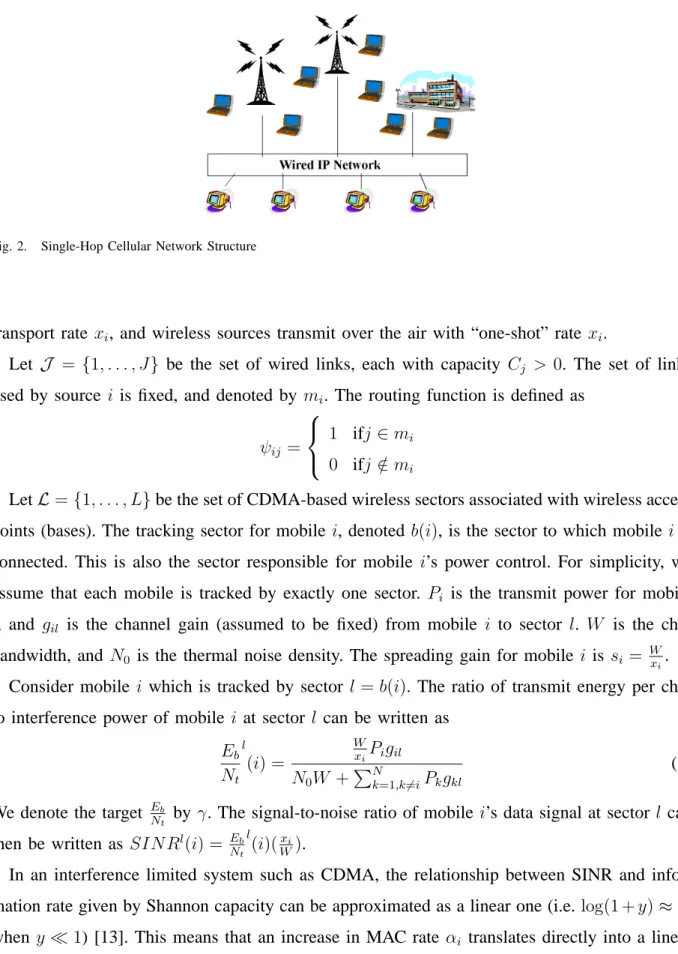
We focus on the uplink of a broadband CDMA network with variable transmission rates, similar to cdma 1xEVDO systems. Mobiles communicate directly with the base stations, which are connected directly to the wired IP network, as shown in Figure 2.
Let N ={1, . . . , N, N + 1, . . . , M} be the set of all sources, where the first N are wireless sources (also referred to as mobiles). Wired sources transmit over the wired network with
Fig. 2. Single-Hop Cellular Network Structure
transport rate xi, and wireless sources transmit over the air with “one-shot” rate xi.
Let J = {1, . . . , J} be the set of wired links, each with capacity Cj > 0. The set of links used by source i is fixed, and denoted by mi. The routing function is defined as
ψij = 1 ifj ∈mi 0 ifj /∈mi
LetL ={1, . . . , L}be the set of CDMA-based wireless sectors associated with wireless access points (bases). The tracking sector for mobile i, denoted b(i), is the sector to which mobile i is connected. This is also the sector responsible for mobile i’s power control. For simplicity, we assume that each mobile is tracked by exactly one sector. Pi is the transmit power for mobile
i, and gil is the channel gain (assumed to be fixed) from mobile i to sector l. W is the chip bandwidth, and N0 is the thermal noise density. The spreading gain for mobile i is si = Wxi.
Consider mobile i which is tracked by sector l =b(i). The ratio of transmit energy per chip to interference power of mobile i at sector l can be written as
Eb Nt l (i) = W xiPigil N0W + PN k=1,k6=iPkgkl (1) We denote the target Eb
Nt by γ. The signal-to-noise ratio of mobile i’s data signal at sector l can then be written as SIN Rl(i) = Eb
Nt l
(i)(xi W).
In an interference limited system such as CDMA, the relationship between SINR and infor-mation rate given by Shannon capacity can be approximated as a linear one (i.e. log(1 +y)≈ y when y¿1) [13]. This means that an increase in MAC rate αi translates directly into a linear increase in information rate if and only if Eb
assume the condition Eb
Nt =γ is necessary for decodability of transmissions at a rate proportional toxi [14]. In order to ensure the validity of the approximationlog
³ 1 + Eb Nt l (i)(xi W) ´ ≈ Eb Nt l (i)(xi W), we introduce the following technical assumption which is consistent with practical systems [15].
Technical Assumption 1: The target value Eb
Nt =γ must satisfy γ <4.
A. Cross-Layer Optimal Rate Assignments
In order to address rate control as a constrained optimization problem, we must first introduce the notion of feasible rate assignments. In a wired network, a feasible rate assignment is typically one in which sum rate of all users transmitting across a given link is less than the capacity of the link. In a wireless network, however, the definition of what constitutes a feasible rate-power pair is highly dependent upon the design of a particular system. Constraints may include minimum or maximum power constraints, interference limits, minimum rate guarantees, QoS metrics, or maximum delay requirements. Since the focus of this work is a CDMA DO network, we use a common definition of feasible MAC rates which depends on both a target Eb
Nt (denoted by γ), and a target interference level (denoted by K). A more detailed explanation of these feasibility criteria can be found in the 3GPP2 standards for CDMA2000 [16].
We say a rate vector x= (x1, . . . , xM) is feasible if there exists a non-negative power vector (P1, . . . , PN) such that the following conditions are satisfied:
C1. PMi=1xiψij ≤Cj ∀j ∈ J C2. Eb Nt l (i)≥γ ∀i≤N and l =b(i) C3. PNi=1Pigil ≤KN0W ∀l ∈ L C4. 0≤xi ≤ W4 ∀ i≤N
where γ and K are constants. The first condition is the link capacity constraint for the wired network [4], and depends on the routing matrix ψ. The second condition specifies the target
Eb
Nt level, while the third conditions specifies a limit on the ratio of received power to thermal noise at each base station1. Together, these two conditions guarantee an acceptable BER for
wireless transmissions. The last condition simply ensures the validity of the standard Gaussian 1Such a condition is often used to help maintain stability of the system (see [6], [16], [17], for further discussion).
approximation used for performance analysis of a matched filter receiver2.
In [17] and [20], we have developed a simpler feasibility region with a linear-type structure. Using similar modifications, we formally define our feasibility region.
Definition 1: A rate vector x= (x1, . . . , xM) belongs to the feasible region ∆ if and only if
it satisfies the following conditions: LC1. PMi=1xiψij ≤Cj ∀ j ∈ J LC2. PNi=1 xi W+γxi gil gib(i) ≤ K γ(1+K) ∀ l ∈ L LC3. 0≤xi ≤ W4 ∀ i≤N
Condition LC2 is obtained by considering Condition C3 as an equality, solving for the transmis-sion powers, and substituting into Condition C2. In Theorem 3 in [17], we have shown that if
α∈ ∆ then it satisfies Conditions C1-C4. In general, the region defined by ∆ will be a subset of that defined by C1-C4. We have provided a detailed discussion on the relationship between ∆ and the feasibility region defined by C1-C4 in [17].
Among all feasible rate vectors, we wish to choose a rate vector that is proportional fair [1]. In other words, we choose to optimize the utility function PMi=1log(xi), resulting in the following problem:
Problem P
Find the rate vector x that is the solution to:
x∗ = arg max x∈∆ M X i=1 log(xi)
It is worth noting that the results presented in this paper can be extended to more general utility functions with minimal modifications to the problem setup.
III. DISTRIBUTED ALGORITHM FORRATEASSIGNMENTS
In the remainder of this paper, we see how optimization and dual methods can be used to design distributed algorithms that converge to the cross-layer optimal solution to Problem P. The challenge in directly applying dual methods to Problem P is that ∆ is not a convex region. In 2An important (and often neglected) issue in high data rate CDMA networks is the performance degradation due to
multi-path interference when low spreading gains are used [18], [19]. Thus, we restrict our attention to transmission rates that result in spreading gains that the authors in [18] have shown to exhibit only moderate performance degradation due to multi-path interference.
order to remedy this, we introduce the change of variable ri = xiγx+iW. This gives the following problem, which we show to be a convex problem with no duality gap.
Problem P1 max 0≤r≤ 1 γ+4 M X i=1 log( riW 1−γri ) s.t. M X i=1 riW 1−γri ψij ≤Cj ∀ j ∈ J N X i=1 ri gil gib(i) ≤ K γ(1 +K) ∀ l∈ L
Theorem 1: Problem P1 is a convex optimization problem for which there is no duality gap. Proof: It is simple to verify that under Technical Assumption 1, the objective function in
Problem P1 is strictly concave and the constraints are convex over the range 0 ≤ ri ≤ γ+41 . From Proposition 5.3.1 (page 512) in [21], we know that there is no duality gap if there exists a vector of primal variables r such that
M X i=1 riW 1−γri ψij−Cj <0 ∀ j ∈ J and N X i=1 ri gil gib(i) − K γ(1 +K) <0 ∀ l∈ L This is clearly satisfied with ri = 0 ∀i= 1, . . . , M and we are done.
We now consider the Lagrange function associated with Problem P1: L1(r, λ, µ) = M X i=1 log( riW 1−γri )− J X j=1 λj à M X i=1 riW 1−γri ψij −Cj ! − L X l=1 µl à N X i=1 gil gib(i) ri − K γ(1 +K) !
The dual problem can be formulated as follows:
DP1. Find the Lagrangian multipliers (λ1, . . . , λJ) and (µ1, . . . , µL) such that they solve min µ,λ≥0 M X i=1 φi(qi, pi) + J X j=1 λjCj+ K γ(1 +K) L X l=1 µl
where qi = J X j=1 λjψij and pi = PL l=1 gibgil(i)µl i= 1, . . . , N 0 i=N + 1, . . . , M and φi(qi, pi) = max r µ log( riW 1−γri )− r 1−γrqi−rpi ¶ (2) Notice that for a given set of Lagrange multipliers, Eqn (2) is an autonomous rule that can be implemented at each source using locally available information. This is an extremely attractive property since it allows for distributed computation of the rate assignments: when the multipliers are chosen appropriately, the autonomous rule given by Eqns (2) results in a globally optimal, proportional fair solution. The remaining task is to generate the correct Lagrange multipliers, which we do using a gradient projection method. Substituting xi back in gives the following algorithm consisting of three parts:
Base Algorithm
Each base station produces a regulatory signal (Lagrangian multiplier µl) that indicates the level of interference at that sector. This signal evolves according to the difference equation:
∆µl = β(PNi=1 gil gib(i) xi W+γxi − K γ(1+K)) if µl(t)>0 β[PNi=1 gil gib(i) xi W+γxi − K γ(1+K)]+ if µl(t) = 0 (3)
where β is a constant and PNi=1 gil gib(i)
xi
W+γxi is a measure of interference at each sector. These signals are then used to generate the aggregate signals p.
Link Algorithm
Each link produces a regulatory signal (Lagrangian multiplier λj) that indicates the level of congestion at that link. This signal evolves according to the difference equation:
∆λj = ξ(PMi=1xiψij−Cj) if λj(t)>0 ξ[PMi=1xiψij−Cj]+ if λj(t) = 0 (4)
where ξ is a constant and PMi=1xiψij is the total traffic on link j. These signals are then used to generate the aggregate signals q.
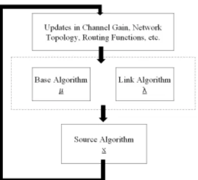
Fig. 3. Control-Theoretic View of Modular Rate Assignments Fig. 4. Flowchart of Algorithm Operation
Each source reacts to the levels of congestion (indicated by the link coordination signals) and, when applicable, the interference levels at its neighboring sectors (indicated by the base coordination signals) by adjusting its rate such that
xi = arg max x µ log(x)−xqi− x W +γxpi ¶ (5) Figure 3 gives a control-theoretic view of the algorithm, while Figure 4 gives a flowchart of algorithm operation. At each update interval, the Base Algorithm and Link Algorithm are run simultaneously, taking into account any changes in network conditions. The Source Algorithm is then run, taking into account the new congestion and interference prices. From these figures, we see one of the main advantages to the type of feedback structure we have employed - when run continuously, the algorithm will 1) converge to the optimal rate allocation, and 2) adapt to quasi-static changes in network conditions.
We now introduce the following convergence theorem, whose proof can be found in Appendix II.
Theorem 2: There exist values β0 and ξ0 such that for all β < β0 and ξ < ξ0, the distributed
algorithm described by Eqns (3)- (5) converges to the solution to Problem P.
IV. PRACTICAL DISTRIBUTEDIMPLEMENTATION
A. Signaling Mechanisms
The computation and communication of regulating signals is the basis of the distributed algorithm described in the previous section. However, Lagrange multipliers need not be locally available, even though they can always be computed in parallel via (in general complicated) message passing schemes as those in [8]. In other words, we distinguish between the above
described parallel implementations, and truly distributed rate control in which locally available observations are used. Throughout this section, we substantiate our claim that our proposed algorithms can be implemented in a distributed manner with reasonable overhead using locally available observations. In particular, we are interested in addressing 1) the computation of the regulating signals µ and the availability of p, and 2) the computation of the regulating signals
λ and the availability of q.
Recall the base algorithm from Eqn (3). This equation requires each base to know information about the load at all other bases. In order to facilitate distributed computation, we introduce the following alternative which approximates the original solution:
∆µlw β(PNi=1 Pigil N0W −K) if µl(t)>0 β[PNi=1 Pigil N0W −K] + if µ l(t) = 0 (6) The quantity PNi=1 Pigil
N0W can be measured at base station l [16], and represents the sector’s
overall interference. This quantity is referred to as Rise Over Thermal (ROT) [16]. Notice that this alternate algorithm does not require an estimate of loading at the other base stations; rather, we use an over-estimation of the load at neighboring base stations by assuming Zl = K ∀ l. Although we do not have analytical results on the equilibrium point when this alternate algorithm is used, such an equilibrium will in general violate the linear constraints LC1-LC3, but will satisfy the original (non-linear) constraints C1-C4 [17]3.
Once the regulating signalsµl are computed at each base, they are used to generate aggregate signals for each mobile. Recall the definition of each user’s aggregate wireless signal pi =
PL
l=1 gibgil(i)µl. At first glance it seems that in order to calculate pi, each mobile requires full
knowledge of the channel. In [17] and [20] we have shown that there exists a practical solution to this problem using the CDMA pilot signal, PS, and a pricing pilot signal, PPS. This pilot symbol is transmitted with a power level proportional to the base signal, µl. Hence pi can be calculated as pi = PL l=1ggibil(i)µl w EP P S T R EP T(b(i)) where E P P S
T R and ETP(b(i)) are quantities which can easily be measured locally by mobile i (see [17] and [20] for more details).
The practical scheme to compute the wired link signals λ and the corresponding aggregate 3
Note that both the original and the modified base algorithms require sources to transmit over the air with rate xi, even
if the queue is not long enough to sustain such a rate. Although wasteful of bandwidth during transient periods, this can be accomplished by transmitting “dummy” packets and will not impact the optimality of the equilibrium point.
signalsqis well understood since Eqn (4) has a well-known interpretation in terms of queue delay at each link [4], [5], [8]. When dealing with a discrete-time system, however, the usual differential equation for queueing delay λ˙j = C1j(
PM
i=1xiψij −Cj) becomes ∆λj = ∆Cjt(
PM
i=1xiψij −Cj),
where ∆t is the time between successive updates. If we set ξ = ∆Cjt, then λj is the queueing delay at link j, and qi is user i’s end-to-end queueing delay. Recall from Theorem 2, however, that the convergence of the algorithm is dependent upon the step-size being “small enough” (see [22], pages 212-215 for further discussion). Since the step size is proportional to the update interval ∆t, the convergence of the modular algorithm is dependent upon the time-scale of the distributed feedback loops shown in Figure 3. In other words, in order to guarantee convergence we must either run the algorithm “fast enough” (small ∆t) or use a scaled version of delay as the feedback signal (use stepsize of SC∆t, S ≥1). The aggregate signals are now the end-to-end delay divided by S, which can still be locally computed by the sources. The drawback is that the
actual delay is nowS times higher than if we had simply run the algorithmS times faster. This
is similar to the concept of tightly and loosely coupled links in [11], where the use of scaling results in loosely coupled links.
B. Simulation Results
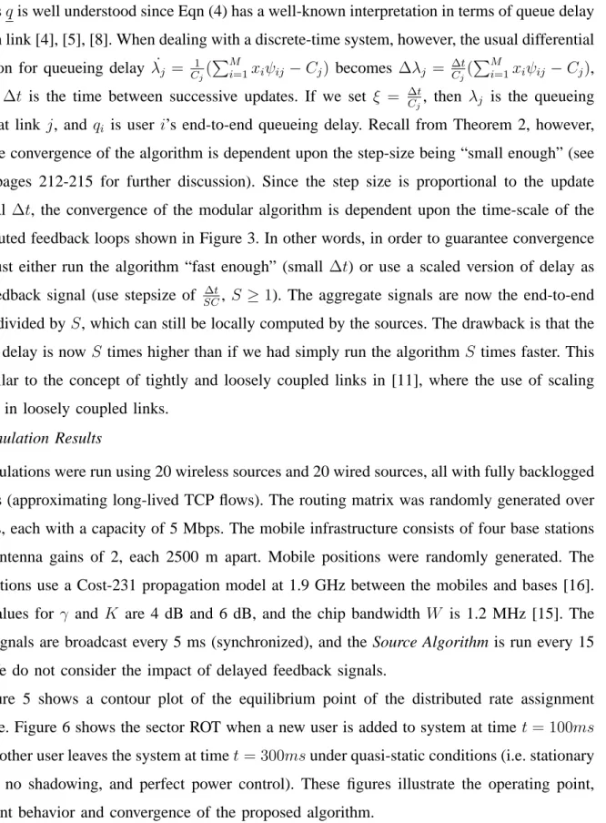
Simulations were run using 20 wireless sources and 20 wired sources, all with fully backlogged buffers (approximating long-lived TCP flows). The routing matrix was randomly generated over 6 links, each with a capacity of 5 Mbps. The mobile infrastructure consists of four base stations with antenna gains of 2, each 2500 m apart. Mobile positions were randomly generated. The simulations use a Cost-231 propagation model at 1.9 GHz between the mobiles and bases [16]. The values for γ and K are 4 dB and 6 dB, and the chip bandwidth W is 1.2 MHz [15]. The PPS signals are broadcast every 5 ms (synchronized), and the Source Algorithm is run every 15 ms. We do not consider the impact of delayed feedback signals.
Figure 5 shows a contour plot of the equilibrium point of the distributed rate assignment scheme. Figure 6 shows the sector ROT when a new user is added to system at time t= 100ms and another user leaves the system at timet= 300msunder quasi-static conditions (i.e. stationary nodes, no shadowing, and perfect power control). These figures illustrate the operating point, transient behavior and convergence of the proposed algorithm.
60 80 100 120 140 160 180 0 1000 2000 3000 4000 5000 0 1000 2000 3000 4000 5000 Distance (m) Distance (m) Mobile Rate (Kbps)
Fig. 5. Contour Plot of Wireless User Rates
0 100 200 300 400 500 4 6 8 10 12 14 16 Time (ms) ROT at Base 1 (dB)
Fig. 6. ROT for Changing Network Topologies
V. CONCLUSIONS ANDFUTURE WORK
In this paper, we have developed a cross-layer approach to optimal rate assignment in multi-sector CDMA networks. We formulated the rate assignments as an optimization problem subject to interference and congestion constraints, and developed distributed algorithms to solve this maximization problem. Finally, we introduce signalling mechanisms and briefly examined the transient behavior of the algorithm.
The cross-layer approach to optimal rate assignment presented in this paper is a “one-shot” algorithm; that is, it combines the MAC and transport layer protocols to control interference and congestion simultaneously. Traditionally, however, MAC and transport layer protocols are implemented separately. An important area of future work is the investigation of “modular”-type algorithms, in which MAC and transport protocols are coordinated, rather than merged, to achieve cross-layer optimal rate assignment. We have begun investigating dual-based algorithms in which the delay associated with addition of intermediate queues at each wireless source provides the necessary information for coordinating MAC and transport layers. We do not yet have analytical results regarding the performance of such algorithms. However, initial simulations suggest that this approach not only allows for modular implementation (hence, the ability to run MAC and transport protocols at different time scales) but provides a level of robustness to channel variation and changes in the network setting.
APPENDIXI: SUPPORTINGDEFINITIONS AND LEMMAS FOR THEOREM2
Fact 1: Given a set of Lagrangian multipliers and the corresponding dual objective function
minimizes D(·) if D(·) is convex, lower bounded, continuously differentiable, and ∇D(·) is Lipschitz continuous (for proof, see [22], pages 213-214).
Definition 2: Let ϕ be a (J +L) by 1 vector containing the Lagrangian multipliers λ and µ
(i.e. ϕT =
h λµ
i
). We can write the dual objective function as
D(ϕ) = M X i=1 φi(qi, pi) + J X j=1 ϕjCj+ K γ(1 +K) L X j=J+1 ϕj where φ(·), qi, and pi are as described earlier in the dual problem, DP1.
Lemma 1: The dual objective function D(ϕ) is lower bounded, convex, and continuously
differentiable over the feasibility region.
Proof: That D(ϕ) is lower bounded and convex comes directly from the properties of
the dual objective function and weak duality [4]. From Proposition 6.1.1 (page 605) in [21], we know that D(ϕ) is continuously differentiable if ∀ ϕ, the Lagrange function L1(r, ϕ) has a
unique maximizer. From Theorem 1, we know that L1(r, ϕ) is a strictly concave function of r.
Since the allowable values of rform a convex set, the functionL1(r, ϕ)has a unique maximizer.
Fact 2: For a given set of Lagrange multipliers ϕ, the rates that uniquely maximize L(r, ϕ)
are given by r∗ i = arg max 0≤r≤ 1 γ+4 µ log( rW 1−γr)− rW 1−γrqi−rpi ¶ (7)
Definition 3: The gradient of the dual objective function is given by the following(J+L)×1
vector (indexed by j): ∇D(ϕ) = Cj− PM i=1 r∗ iW 1−γr∗ iψij K γ(1+K)− PN i=1ri∗ gij gib(i) (J×1) (L×1) (see [22], page 669).
Definition 4: The Hessian of the dual objective function is given by the following (J+L)×
(J+L) matrix (indexed by j,k): ∇2D(ϕ) = PM i=1(1−γrW∗ i)2ψij ∂r∗ i ∂ϕk PN i=1 gij gib(i) ∂r∗ i ∂ϕk
Proof:
From Fact 2 and taking first order conditions, we note that either: 1. ri∗ = γ+41 (a boundary value of (7)), or 2. r∗ 1 i(1−γr∗i) − W (1−γr∗ i)2qi−pi = 0
If r∗i = γ+41 is a boundary value, then limϕk−ϕ0k→0 r∗
i(ϕk)−r∗i(ϕ0k)
ϕk−ϕ0k = 0. Otherwise, we have the following: ∂r∗ i ∂ϕk = (r ∗ i)2 ³ W(1−γr∗ i)∂ϕ∂qik + (1−γr ∗ i)3∂ϕ∂pik ´ (1−γr∗ i)(2γri∗−1)−2γW qi(r∗i)2 (8) We can now upper bound the terms in the Hessian of the dual objective function using (8) by:
∇2D(ϕ) = AJ×J BJ×L CL×J DL×L where AJ×J = hPMi=1 W 2ψ ijψik (1−γr∗ i)h(i) i BJ×L = · PM i=1 W ψijgibgik (i)(1−γr ∗ i) h(i) ¸ CL×J = · PN i=1 Wgibgij (i)ψik(1−γr ∗ i) h(i) ¸ DL×L = · PN i=1 gij gik gib2(i)(1−γr ∗ i)3 h(i) ¸ and h(i) = (1−2γr∗i)(1−γr∗i) (r∗ i)2 + 2γW qi.
Using Technical Assumption 1 and the upper bound ri ≤ γ+41 , we have
1. the numerator of each term in the sum is non-negative and upper bounded by 2W2 for each element of ∇2D(ϕ), and
2. (1−γri∗)(1−2γr∗i)>0
Finally, by definition, qi ≥0∀ i. Thus, each term in the summation is upper bounded for every element of the Hessian. Since the summations are finite, this implies that the summation is also upper bounded for every element of the Hessian, and we are done.
Lemma 3: The Hessian of the dual objective function ∇D(ϕ) is Lipschitz continuous (i.e.
Proof: Using Taylor theorem and norm definitions, we have
k∇D(ϕ)− ∇D(ϕ0)k
2 = k∇2D(ϕ)(ϕ−ϕ0)k2
≤ k∇2D(ϕ)k
2kϕ−ϕ0k2
[4]. Now, using the properties of the norm (see [22], pages 626, 634-635), we can write k∇2D(ϕ)k2 2 = k∇2D(ϕ)∇2D(ϕ)Tk2 ≤ k∇2(D)(ϕ)∇2(D)(ϕ)Tk ∞ · k∇2(D)(ϕ)∇2(D)(ϕ)Tk 1 = k∇2(D)(ϕ)∇2(D)(ϕ)Tk2 1 = (max j J+L X i=1 |aij|)2 where aij are the elements of (∇2(D)(ϕ)∇2(D)(ϕ)T). Thus,
k∇2(D)(ϕ)k ≤max j J+L X i=1 |aij|
Since the elements of ∇2(D)(ϕ) are bounded (as given by Lemma 2), so are the elements of ∇2(D)(ϕ)∇2(D)(ϕ)T. Thus, k∇2(D)(ϕ)kis bounded by some value K, resulting in Lemma 3.
ACKNOWLEDGMENT
The authors would like to thank Dr. C. Lott at Qualcomm Corporate R&D for his thoughtful suggestions. This work was supported in part by the NSF CAREER Award No. CNS-0347961 and in part by the ARO-MURI Grant No. W911NF-04-1-0224.
REFERENCES
[1] F. Kelly, “Mathematical modelling of the Internet,” in Mathematics Unlimited - 2001 and Beyond, B. Engquist and W. Schmid, Eds. Springer-Verlaq, 2001, pp. 685–702.
[2] H. Balakrishnan, S. Seshan, E. Amir, and R. Katz, “Improving TCP/IP performance over wireless networks,” in Proceedings
of the First ACM Conference on Mobile Computing and Networking, 1995.
[3] J. Price and T. Javidi, “Cross-layer (MAC and transport) optimal rate assignment in CDMA-based wireless broadband networks,” in Proceedings of the Asilomar Conference on Signals, Systems and Computers, Nov. 2004, pp. 1044–1048. [4] S. H. Low and D. E. Lapsley, “Optimization flow control, I: Basic algorithm and convergence,” IEEE/ACM Transactions
[5] J. Mo and J. Walrand, “Fair end-to-end window-based congestion control,” IEEE/ACM Transactions on Networking, vol. 8, no. 5, pp. 555–567, Oct 2000.
[6] J. Price and T. Javidi, “On dual methods for adaptive resource allocation in wireless networks: A taxonomy of practical challenges in CDMA,” in Resource Allocation in Next Generation Wireless Networks, Y. Pan and W. Li, Eds., Preprint. [7] L. Chen, S. Low, and J. Doyle, “Joint congestion control and media access control design for ad hoc wireless networks,”
in Proceedings of IEEE INFOCOM, 2005.
[8] M. Chiang, “To layer or not to layer: Balancing transport and physical layers in wireless multihop networks,” in Proceedings
of IEEE INFOCOM, 2004.
[9] T. ElBatt and A. Ephremides, “Joint scheduling and power control for wireless ad hoc networks,” IEEE Transactions on
Wireless Communications, vol. 3, no. 1, pp. 74–85, January 2004.
[10] A. Eryilmaz and R. Srikant, “Fair resource allocation in wireless networks using queue-length-based scheduling and congestion control,” in Proceedings of INFOCOM, 2005.
[11] X. Lin and N. Shroff, “Joint rate control and scheduling in multihop wireless networks,” in Proceedings of the IEEE
Conference on Decision and Control, 2004.
[12] S. Hanly and D. Tse, “Multiaccess fading channels II: Delay-limited capacities,” IEEE Transactions on Information Theory, vol. 44, no. 7, pp. 2816–2831, Nov 1998.
[13] R. Leelahakriengkrai and R. Agrawal, “Scheduling in multimedia CDMA wireless networks,” IEEE Transactions on
Vehicular Technology, vol. 52, no. 1, Jan 2003.
[14] R. D. Yates, “A framework for uplink power control in cellular radio systems,” IEEE Journal on Selected Areas in
Communications, vol. 13, no. 7, pp. 1341–1347, Sept 1995.
[15] P. Black and Q. Wu, “Link budget of CDMA2000 1xev-do wireless Internet access system,” in The 13th IEEE International
Symposium on Personal, Indoor and Mobile Radio Communications, vol. 4, Sept 2002, pp. 1847–1852.
[16] 3rd Generation Partnership Project 2 (3GPP2), “cdma2000 high rate packet data air interface specification,” www.3gpp2.org, Technical Report C.S0024-A v2.0, 2005.
[17] J. Price and T. Javidi, “Decentralized rate assignments in a multi-sector CDMA network,” IEEE Transactions on Wireless
Communications, vol. 5, no. 12, December 2006.
[18] D. Kalofonos and J. Proakis, “On the performance of coded low spreading gain DS-CDMA systems with random spreading sequences in multipath Rayleigh fading channels,” in Global Telecommunications Conference, vol. 6, November 2001, pp. 3247–3251.
[19] K. Hwang and K. Lee, “Performance analysis of low processing gain DS/CDMA systems with random spreading sequences,” IEEE Communications Letters, vol. 2, no. 12, pp. 315–317, December 1998.
[20] J. Price and T. Javidi, “Decentralized and fair rate control in a multi-sector CDMA system,” in Proceedings of the Wireless
Communications and Networking Conference, 2004.
[21] D. Bertsekas, Nonlinear Programming. Athena Scientific, 1999.