A Competitive and Dynamic Pricing Model for
Secondary Users in Infrastructure based Networks
Soumitra Dixit, Shalini Periyalwar, and Halim Yanikomeroglu
Broadband Communications and Wireless Systems (BCWS) Centre,Department of Systems and Computer Engineering, Carleton University, Ottawa, Ontario K1S 5B6, Canada. E-mail:{sdixit, shalinip, halim}@sce.carleton.ca
Abstract—Enabling unsubscribed Secondary User (SU) access
through Dynamic Spectrum Access (DSA) techniques provides a huge opportunity to the Wireless Service Providers (WSPs) for achieving efficient radio spectrum usage as well as gain additional profits. This paper presents a novel and dynamic SU pricing model for implementation by the WSPs at their Base Stations (BSs) based upon a BS-centric distributed framework, that allows the SU price to vary dynamically with the changing radio spectrum usage at the BS. Assuming high competition among regional WSPs, a non-cooperative competition structure is considered among the WSPs, where neither information nor resources are shared among the WSPs. A simple single cell scenario easily scalable to multiple cells achieving competitive yet dynamic SU pricing among the BSs of two WSPs, is presented in this paper. The final SU price is seen to depend on the spectrum utilization at the BS, the wireless channel, and the price charged by WSPs to their Primary Users (PUs).
I. INTRODUCTION
Unbalanced utilization of the radio spectrum with respect to time and location coupled with huge investments by the Wireless Service Providers (WSPs) in acquiring the licensed spectrum, have a serious impact on the bottom line of the WSPs, and in turn on the price paid by the subscribers for wireless access. Enabling temporary wireless access to Secondary Users (SUs) through Dynamic Spectrum Access (DSA) techniques, provides the WSPs with an opportunity to not only improve the efficiency of radio spectrum usage but also earn additional profits from such SU access [1], [2].
To this effect, majority of the work in literature has focused on spectrum sharing techniques and SU pricing models based on a centralized approach, where a Centralized Mediating Entity (CME) such as a spectrum broker or a spectrum regulator pools the unutilized spectrum information from all the WSPs in the area [1], [3]–[5]. This approach is envisioned to regulate, co-ordinate and lease the spectrum temporarily (hours) to either WSPs interested in temporarily increasing their capacity [3], [4], or directly to SUs requiring temporary wireless access [5], [6].
However, two primary difficulties can be foreseen con-sidering the implementation of the centralized approaches described above involving CMEs. Firstly, radio spectrum usage characteristics are observed to vary with respect to time and location, thus leading to the requirement of multiple regional CMEs with increased signaling overhead for CME-WSP coor-dination. Secondly, considering the highly competitive
multi-WSP environment, it can be considered unlikely for the multi-WSPs to share their spectrum or spectrum related information.
In this paper, we present a methodology to implement the Base Station (BS)-centric distributed framework from [2] for achieving competitive yet dynamic SU pricing among the WSPs in a region, while simultaneously maximizing individual WSP profits from SU access. Since the analysis in this paper is based on the BS-centric distributed framework from [2], the individual WSPs are assumed to operate without the presence of CMEs, and in a non-cooperative manner without any sharing of spectrum or spectrum related information. It must be noted that, the BSs are considered to be independent elements setting SU prices based on their local spectrum utilization, and act in the best interest of their respective WSPs. The organization of this paper is as follows: Section II intro-duces the BS-centric distributed framework and the dynamic incentive based SU pricing model [2]. Section III describes the methodology for achieving profitable yet competitive dynamic SU pricing among the WSPs in the area, without inter-WSP cooperation. Simulations and results showcasing the profitabil-ity potential to the WSPs from such SU access are presented in Section IV, with Section V highlighting the conclusions.
II. BS-CENTRICDISTRIBUTEDFRAMEWORK AND
DYNAMICSU PRICING
The BS-centric distributed framework [2] implemented in this paper considers enhanced BSs with the capability of providing direct temporary SU access, by conducting SU admission control and Primary User (PU)-SU resource allo-cation decisions based on their instantaneous spectrum usage characteristics. This distributed framework not only improves the instantaneous spectrum usage, but also reduces the heavy signaling overhead required in CME-WSP-BS coordination.
Every BS in this distributed framework broadcasts their lo-cal spectrum information (e.g., SU price per application class) to the SUs in the area. The SUs can therefore select the most-suitable BS and potentially acquire temporary wireless access instantaneously directly from the BS, rather than waiting for the CME to negotiate and select a WSP, which in turn selects the most suitable BS to provide access to the SU. It must be noted that, the BS-centric distributed framework [2] allows temporary wireless access to SUs, if and only if, there remain surplus spectrum available at the BS after the all PUs (i.e.,
^ŽĨt^Wϭ ;tŝDyͿ ^ŽĨt^Wϯ ;>dͿ ^ĞůĞĐƚĞĚ^ ^h ^ŽĨt^WϮ ;>dͲͿ >ŽĐĂůƐƉĞĐƚƌƵŵ ŝŶĨŽƌŵĂƚŝŽŶ^ĺ^h ^ƉĞĐƚƌƵŵĂĐĐĞƐƐ ƌĞƋƵĞƐƚ^hĺ%6 WhƵƚŝůŝnjĂƚŝŽŶ ĂƚƚŚĞ^ ŝ͕ƉƵ ^ƉĞĐƚƌƵŵ ĂǀĂŝůĂďůĞĂƚ ƚŚĞ^ĨŽƌ^hƐ ŝ͕ƉƵ ^ƉĞĐƚƌƵŵďĂŶĚůŝĐĞŶƐĞĚďLJ ƚŚĞt^WĂǀĂŝůĂďůĞĂƚƚŚĞ^ ;^ŝŶŐůĞĨƌĞƋƵĞŶĐLJŶĞƚǁŽƌŬͿ
Fig. 1. Distributed framework for SU access [2]
subscribers) have been satisfactorily served, thus guaranteeing no disruption to PU service.
Figure 1 illustrates the BS-centric distributed framework based scenario, where a SU can potentially gain temporary wireless access from the BS of one of the three WSPs. The WSPs are assumed to have a single frequency network with an all-IP framework, where the unutilized spectrum at each BS can be made available to the SU in its coverage area.
A. Terminology: SU Pricing Model
Assuming the total spectrum at the BS to be 1 unit, the frac-tion of the spectrum utilized by PUs at BSiis denoted byαi,pu, while the unutilized spectrum available to the SUs is given by (1−αi,pu), as shown in Fig. 1. The variable price charged to the SUs by the BSs (WSPs) for a particular application class (finite time t in seconds: delay sensitive applications, finite block of B bytes: delay insensitive applications) is known as the SU price and denoted by si. The fixed price charged by the WSPs to the PUs for the same application class is referred to as the PU price denoted by pi.
Before detailing the SU pricing model, the terminology relevant to spectrum utilization at BSi is listed as follows:
αi,pu :PU utilization or PU demand at BSi,
αi,h :Spectrum reserved (handoff and overload protection),
αi,th :Threshold for spectrum utilization; αi,th = 1−αi,h,
αi,su :SU utilization; αi,su exists iff αi,pu< αi,th,
αi,t :Spectrum Utilization Factor (SUF), i.e.,αi,pu+αi,su,
αi,ic :Incentive cutoff limit beyond whichsi> pi,
whereαi,pu, αi,h, αi,th, αi,su, αi,t, αi,ic ∈ [0,1].
B. Dynamic Incentive based Pricing Model
The SU price si is defined in terms of the fixed PU price
pi and the SUF at the BS can be given as [2]
si= (fi(αi,t))mi×pi, (1) where si,fi(αi,t),pi andmi are non-negative real numbers.
The termfi(αi,t)is the normalized SU price with respect to (w.r.t.) the fixedpiand captures the variable nature of spectrum utilization at the BS. This term based on the log barrier function [7], and has an inherent property for SU admission admission control. The normalized SU price is defined as
fi(αi,t) = ⎧ ⎨ ⎩ −ln 1− αi,t αi,th ni if αi,t< αi,th ∞ if αi,t≥αi,th , (2) where ni is a positive real number representing the Incentive Cutoff Factor (ICF). The ICF is useful in defining the incentive in (2), such that whenαi,t< αi,ic, we havesi< pi. The value of ICF is be obtained by solving (2) setting αi,t =αi,ic and
fi(αi,t) = 1 [2]. This incentive structure embedded into the
SU pricing model, depends on the PU price, and allows the WSPs to attract more SUs during periods of low PU demand (off-peak hours) and discourages the SUs to join the network during periods of high PU demand (peak hours).
The exponent of fi(αi,t) in (1) is a non-negative real number referred to as the Price Leveling Factor (PLF) denoted by mi, and provides additional flexibility to the WSPs for pricing the SUs. The PLF is used in the next section to set SU prices with the aim of maximizing individual WSP profits, considering inter-WSP competition and SU pricing incentives. Assumingαi,pu < αi,ic, Fig. 2 shows the dynamic nature of the pricing model for BSiwith the configuration parameters
αi,ic= 0.7 andαi,th = 0.9. The original SU price with PLF
mi = 1is denoted by si, while the new adjusted SU pricing curve with PLFmi = 1is denoted assi in Fig. 2. The profits from SUs can be demonstrated comparing the PLF mi = 1 andmi= 0.3, with the latter assuring profits to the WSP for every SU served considering a fixed costC.
The pricing model [2] above can be described as dynamic and opportunistic. Dynamic nature of the pricing model can be attributed to the SU price changing w.r.t. the SUF at the
0 0.1 0.2 0.3 0.4 0.5 0.6 0.7 0.8 0.9 1 0 0.5 1 1.5 2 2.5 3 3.5 4 SUF ( αi,t )
SU price (per SU)
s
i
si : mi = 1 si’ : mi = 0.3
Fixed PU price (per PU): pi = 1
Fixed cost (per PU/SU): ci = 0.45
Spectrum at BSi
currently available for SU access
(αi,pu , αi,th )
Inherent SU admission control
si→∞
when αi,t→αi,th
Spectrum at BSi
currently occupied by PUs
αi,pu = 0.4 Spectrum at BS i reserved for handoff and overload protection αi,h =0.1 Spectrum at BSi
currently available with monetary incentive to the SUs
(αi,pu , αi,ic )
Fig. 2. Incentive based dynamic model for SU pricing [2] WSP configuration parametersαi,ic= 0.7, αi,th= 0.9
BSi. The SU pricing structure is calculated at BSi using (1) for a fixed time window T (e.g., 10 minutes) based on the predicted PU demand, and is then broadcasted to the SUs in the area. The SUs gaining access during this time window are priced opportunistically with the SU price being the lowest for the first SU and incrementing for every subsequent SU.
C. Multiple WSPs and Competitive Pricing
Considering PU service, the PUs pay a fixed price (per month, minute, bytes) for a given service (e.g., voice or data) to the WSPs. With multiple WSPs competing (no cooperation among WSPs) for a larger subscriber base, the PU prices set by each WSP can be seen to stabilize and fall into equilib-rium, thus maximize individual WSP profits and providing no incentives to the WSPs for deviating from the set prices [8].
Efficient spectrum utilization requires the WSPs not only to maximize their subscriber base (PUs), but also attract SUs to gain temporary access to the unutilized spectrum at their respective BSs. The WSPs would thus would compete with each other in a non-cooperative manner, with the goal of setting SU prices to maximize their individual profits from SU access. The dynamic SU pricing model allows the WSPs to provide incentives in price to attract the SUs during periods of low SUF, i.e., αi,pu< αi,t< αi,ic.
Although the PLF (mi) provides flexibility to the WSPs to adjust their SU prices, obtaining equilibrium pricing among the WSPs with dynamically changing prices could be prohibitively complex. Therefore a methodology for achieving inter-WSP competitive yet dynamic SU pricing is developed in the next section, based on the linear city model and static SU pricing.
III. NON-COOPERATIVECOMPETITIVESU PRICING
Assuming the BSs as individual entities acting on behalf of their respective WSPs, we consider a single cell scenario to initially find equilibrium SU prices considering static SU pricing. Calculation of these static equilibrium SU prices based on the linear city model will be the intermediate step in achieving non-cooperative competitive dynamic SU pricing.
A. Linear City Model
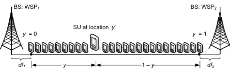
The linear city model assumes a city to be represented by a line of distance 1 unit with a single BS for each of the two competing WSPs placed on either side of the city, as shown in Fig. 3. Since each of the two WSPs in the linear city scenario have only one BS, the same indexiwill be used for the WSPs, beyond this point in the paper. The unit distance on the linear city is represented byy ∈[0,1], and the BSs are assumed to be at a distance dfi from the city, where dfi is the exclusion region and depends on antenna configurations at the BS of WSPi. Hence the linear city extends fromdf1 (y = 0) to the
cell edge (y= 1) for WSP1and vice versa for WSP2. For static SU pricing structure, we assume a fixed SU price
Sito be charged by the WSPs to all the SUs, such that the SUs have a monetary incentive w.r.t. the PU price, i.e., Si < pi. The cost to each WSP for providing temporary wireless access to a single SU is assumed to be fixed and equal C =C1 =
±\ \ %6:63 %6:63 68DWORFDWLRQµ\¶ \ \ GI GI
Fig. 3. SU service differentiation based on the linear city model
C2. Thus from the profitability perspective of the WSPs, the equilibrium SU priceSi∗ must satisfyCi < Si∗ < pi. It must be noted that the SU prices (S1, S2) are assumed to be set
simultaneously by the WSPs with the goal of individual profit maximization, without inter-WSP cooperation.
Price based competition among multiple sellers (i.e. WSPs) theoretically leads to equilibrium prices equaling to the costs, i.e.,Si∗=Ci, thus resulting in zero profits to the sellers [8], [9]. However, such a phenomenon is rarely observed in real markets, since the sellers always distinguish their service based on quality, brand, promotional offers, etc.. The differentiation of their own service from similar service by other WSPs in the region, creates a niche market for the WSPs, maximizing their individual profits as well as competing on prices.
The methodology for achieving competitive inter-WSP SU pricing is thus based on this intermediate step of fixed equilib-rium pricing analysis with SU service differentiation based on the linear city model. The PLF (mi) introduced in Section II can then be used to transform the fixed equilibrium SU prices into competitive yet dynamic SU prices.
A total of q SUs are assumed to be uniformly distributed along the linear city from 0 to 1, and each SU is required to select either of the two WSPs for temporary access. The BSs of the two WSPs are assumed to have sufficient unutilized spectrum in total for serving all the SUs on the linear city.
From the SU’s perspective, selection of a WSP not only depends on the price but also on the signal strength at the SU terminal. Therefore the perceived price (monetary unit: ‘$’) for a SU located at any point ‘y’ can be given as [9]
Ui(y) =Si+ (ζ×y) ($), (3) where ζ is a constant nonnegative real number representing the dissatisfaction level of a SU. Observing (3), the perceived price to the SU for access to the BS of WSPi and hence the dissatisfaction level can be seen to increase asy increases.
B. SU Dissatisfaction Levelζ
In order to define the SU dissatisfaction levelζ in (3), we first define the Satisfaction Level (SL) denoted by τi for the SUs w.r.t. the BS of WSPi. The SL τi(r) for the rth SU on the linear city w.r.t. the BS of WSPi is defined in terms of the spectral efficiencyηi(r)at the SU terminal as
τi(r) =maxηi((r)
ηi). (4)
Averaging out the shadowing, the maximum value of the spectral efficiency ηi can be observed at dfi, i.e., at y = 0
nearest to BS of WSPi. The standard deviation of the SLs from (4) is denoted by σi, and can be used to represent the wireless channel on the linear city. The dissatisfaction level
ζ can be considered as the reciprocal of the SL and can be defined as: ζ=K1K2 ($), whereK1=Δ(1 K2) ($)andK2= σ1+σ2 2 . (5) K1 andK2 are constants and nonnegative real numbers, and
Δ(K2) defines the unit change in the value of K2. With ζ
defined, we now proceed to calculate the equilibrium SU prices with a static SU price (Si) and fixed equal costC.
C. Equilibrium Analysis: Static SU Pricing
For any SU located at a distance y from BS of WSP1 as shown in Fig. 3, the SU will select WSP1 if UW SP,1(y) <
UW SP,2(1−y), while it will select WSP2 if UW SP,1(y) >
UW SP,2(1−y), and in case UW SP,1(y) = UW SP,2(1−y)
either of the two WSPs is randomly selected [9].
It could be possible for WSP1 to capture the entire market by settingS1such thatS1< S2−ζ, i.e., serve all theqSUs in the linear city. However, in context of the system framework and the assumptions described, due to limited quantity of spectrum in offer for the SUs, the entire SU demand cannot be satisfied by a single WSP. Also WSP1 would need to know the SU price S2 set by WSP2, which is contrary to
our assumptions that SU prices are set simultaneously. Therefore, to achieve competitive SU pricing, the WSPs will need to set their SU prices close to each other. From the SUs’ perspective, the SUs will prefer to obtain access from the WSP with the lower SU price, since the SUs cannot be guaranteed Quality of Service (QoS) at all times as the BSs are required to allocate resources to satisfactorily serve the PUs first [2]. With the SU prices set to be close (or equal) to each other by the WSPs, the SUs will prefer to select the WSP with the lower perceived price thus gaining a higher SL.
We now focus on a SU located at a distancedon the linear city, such that UW SP,1(d) = UW SP,2(1−d). Solving the
equality ford, gives us the SU demand at WSP1 as
D1(S1, S2) =ζ−S21+S2
ζ , (6)
where D1(S1, S2) is a nonnegative real number. The profit
achievable by WSP1 based on SU demand can be given as
π1(S1, S2) =S1×(D1(S1, S2))−C×(D1(S1, S2)), (7) where π1(S1, S2) is a nonnegative real number. For profit
maximization, WSP1’s best response to the SU price set by WSP2 can be obtained as
BR1(S2) = ∂π1
∂S1 =
S2+ζ+C
2 . (8)
The model being symmetric for both the WSPs, a similar set of results can be obtained for WSP2. Thus assumingS1=S2,
the Nash Equilibrium (NE) SU price can be expressed as
S∗=C+ζ, (9)
where S∗ is non-negative real number [9].
D. Transformation to Dynamic SU Pricing
The PLF [2] described in Section II provides additional price adjustment flexibility to the incentive based dynamic pricing model, and therefore can be used to transform the static NE SU price into dynamic yet competitive SU pricing.
To implement the transformation, initially, the SU price to be paid by the first SU is adjusted to be equal to the static NE SU price obtained from (9). The value of the PLF is obtained next by rearranging (1) and settingsi =S∗i andαi,t=αi,pu. Finally, the PLF is substituted in (1) to obtain the new dynamic yet competitive SU pricing structure denoted bysi.
Thus it can be observed that incremental SU prices are charged to every new SU, depending upon the amount of unutilized spectrum available at the BS. Since the NE SU price is adjusted to be equal to SU price of the first SU and every subsequent SU pays a higher SU price, the WSPs are guaranteed profits from every SU.
IV. SIMULATIONS ANDRESULTS
For analyzing the profitability potential for the WSPs, a single cell with no inter-cell interference is assumed for the linear city. The wireless channel is based on the urban macro-cell scenario [10], and the simulation parameters are defined in Table I. The carrier frequency of 2 GHz for WSP1and 1.9 GHz for WSP2 is assumed giving a path loss of P L1 = 128.1 +
37.6 log10(δ) andP L2 = 127.7 + 37.6 log10(δ)respectively,
where δis the distance in meters. Every SUs entering BSi is randomly allocated either 400, 500 or 600 KHz, assuming the total bandwidth at BSi to be 20 MHz.
The simulation scenario considered in this paper assumes similar PU utilization at the BSs of the two WSPs and with symmetric incremental WSP costs. However, it must noted that, other scenarios with dissimilar PU utilization and asymmetric WSP costs can also be shown to achieve high inter-WSP competitive pricing.
The competitive nature of the dynamic SU prices can be quantified using the following inter-WSP competitiveness metric:
ψs1,s2 =VAR(Λ),where Λ =|sˆ1−sˆ2|, (10)
and VAR denotes the variance.ˆs1={s1(1), s1(2), ..., s1(L1)}
and sˆ2 = {s2(1), s2(2), ..., s2(L2)} give the vector of the
TABLE I SIMULATIONPARAMETERS
Parameter WSP1 or WSP2
BS-cell edge distance 250 m
Exclusion distancedfi 35 m
BS total transmit power 46 dBm
BS transmitter antenna gain 14 dB SU terminal receiver antenna gain 0 dB
Noise figure 5 dB
Noise power density at SU terminal -174 dBm/Hz
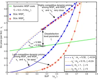
0 0.1 0.2 0.3 0.4 0.5 0.6 0.7 0.8 0.9 0 0.1 0.2 0.3 0.4 0.5 0.6 0.7 0.8 0.9 1 Symmetric WSP costs C = 0.2 + 0.3(αi,t ) SUs: WSP1 SUs: WSP2 SUF (αi,t )
SU price (per SU)
s i s1’ : m1 = 0.32, ζ =0.24 s2’ : m2 = 0.15, ζ =0.24 s1: m1 = 1, ζ = 0 s2: m2 = 1, ζ = 0 Dissatisfaction level parameter ζ α1,pu = 0.365 α2,pu = 0.355
Less competitive dynamic pricing
among WSP1 and WSP2
s1 and s2 far apart
Highly competitive dynamic pricing
among WSP1 and WSP2
s1’ and s2’ very close
Fig. 4. Competitive nature of SU pricing among WSP1and WSP2 WSP configuration parameters specified in Table II
original SU prices set by WSP1and WSP2respectively, while the vector of the new SU prices is given bysˆi. Positive integers
L1andL2 represent the number of SUs served by the WSP1
and WSP2 respectively. Since either L1 ≥ L2 or L1 ≤ L2
such that q=L1+L2, we concatenate eithersˆ1 or sˆ2 such
that L1=L2 before using them in (10).
The competitive nature with dynamic SU pricing can be observed in Fig. 4, with the new SU price (si) curves for both WSPs seen to be very close to each other, in comparison to the original SU price (si) curves. The lower value of the metric
ψs
1,s2 for the new SU prices w.r.t.ψs1,s2 for the original SU
prices as in Table II, validates the competitive nature of the new SU prices. High inter-WSP competition and Cumulative Profits (CP) for the new SU prices can be seen in Fig. 5.
It must be noted that the SU profit results shown in table II and Fig. 5 consider only one BS for the time window T,
0 2 4 6 8 10 12 14 16 −3 −2 −1 0 1 2 3 4 5 6
Number of SUs with wireless access and monetary incentive
Cumulative profits ($) over the time window
T minutes s1’ : m1 = 0.32, ζ =0.24 s2’ : m2 = 0.15, ζ =0.24 s1: m1 = 1, ζ = 0 s2: m2 = 1, ζ = 0
Complete loss for WSP2
Partial profits to WSP1
Highly competitve cumulative profits
for WSP1 and WSP2
Less competitve cumulative profits
for WSP1 and WSP2
Fig. 5. Cumulative profits to WSPs from SUs WSP configuration parameters specified in Table II
TABLE II
WSP PARAMETERS ANDRESULTS
Parameter WSP1 WSP2
PU utilizationαi,pu 0.365 0.355
Spectrum thresholdαi,th 0.9 0.85
Incentive cutoff limitαi,ic 0.7 0.75
Incentive cutoff factorni 1.83 3.67
Results WSP1 WSP2
Number of SUs served with monetary incentive 13 15
CP withζ= 0.24($) 4.95 5.71
% rise in CP forsiw.r.t.si 79.53 129.54
Competitiveness ψs
1,s2: 3.44×10
−4 ψs1,s2: 5.24×10⁻²
and SUs joining the network only when incentives in prices are available. However, this model can be easily scaled to estimate the overall daily SU profit to the WSPs, by simply multiplying the SU profits obtained from a single BS in a day with the total number of BSs owned by the WSP.
V. CONCLUSIONS
This paper provides a methodology for achieving non-cooperative competitive yet dynamic SU pricing, based on a novel BS-centric distributed framework. The framework and methodology described in this paper demonstrates the profitability potential to the WSPs from SU access based on the distributed framework. The final competitive dynamic SU price set by the BS for direct temporary wireless access to the SUs can be observed to depend upon the wireless environment, the SUF at the BS, current PU demand and the PU price.
REFERENCES
[1] T. Weiss and F. Jondral, “Spectrum pooling: an innovative strategy for the enhancement of spectrum efficiency,” IEEE Communications Magazine, vol. 42, no. 3, pp. S8–14, March 2004.
[2] S. Dixit, S. Periyalwar, and H. Yanikomeroglu, “A distributed framework with a novel pricing model for enabling dynamic spectrum access for secondary users,” inProc. IEEE VTC 2009-Fall.
[3] M. Buddhikot, P. Kolodzy, S. Miller, K. Ryan, and J. Evans, “Dimsum-net: new directions in wireless networking using coordinated dynamic spectrum,” inProc. of WoWMoM, June 2005, pp. 78–85.
[4] D. Niyato and E. Hossain, “Microeconomic Models for Dynamic Spectrum Management in Cognitive Radio Networks ,” in Cognitive Wireless Communication Networks, E. Hossain and V.K. Bhargava, Ed. US: Springer, 2007, pp. 391-423.
[5] O. Ileri, D. Samardzija, and N. Mandayam, “Demand responsive pricing and competitive spectrum allocation via a spectrum server,” in Proc. IEEE DySPAN 2005, pp. 194–202.
[6] J. Perez-Romero, O. Salient, R. Agusti, and L. Giupponi, “A novel on-demand cognitive pilot channel enabling dynamic spectrum allocation,” inProc. of IEEE DySPAN, April 2007, pp. 46–54.
[7] S. Boyd and L. Vandenberghe,Convex Optimization. Cambridge, U.K: Cambridge University Press, 2004.
[8] R. Barnes,Economic Analysis, An Introduction. London, U.K: Butter-worth & Co. Ltd., 1971.
[9] B. Polak,Game Theory Lecture Notes. Yale University open courses, 2007. [Online]. Available: http://oyc.yale.edu/economics/game-theory/ [10] 3GPP TR 36.942 v1.2.0, “E-UTRA Radio Frequency (RF) system
![Fig. 1. Distributed framework for SU access [2]](https://thumb-us.123doks.com/thumbv2/123dok_us/1063499.2641319/2.918.82.447.86.326/fig-distributed-framework-for-su-access.webp)