Spatial effects of video compression on classification in convolutional neural networks.

AUTHOR(S):

TITLE:

YEAR:

Publisher citation:

OpenAIR citation:

Publisher copyright statement:

OpenAIR takedown statement:

This publication is made freely available under ________ open access.

This is the ___________________ version of proceedings originally published by _____________________________

and presented at ________________________________________________________________________________

(ISBN __________________; eISBN __________________; ISSN __________).

This publication is distributed under a CC ____________ license. ____________________________________________________

Section 6 of the “Repository policy for OpenAIR @ RGU” (available from

http://www.rgu.ac.uk/staff-and-current-students/library/library-policies/repository-policies

) provides guidance on the criteria under which RGU will

consider withdrawing material from OpenAIR. If you believe that this item is subject to any of these criteria, or for

any other reason should not be held on OpenAIR, then please contact

[email protected]

with the details of

the item and the nature of your complaint.

GREEN

JOHNSTON, P., ELYAN, E. and JAYNE, C.

Spatial effects of video compression on classification in convolutional neural networks.

2018

JOHNSTON, P., ELYAN, E. and JAYNE, C. 2018. Spatial effects of video compression on classification in convolutional neural networks. In Proceedings of the International joint conference on neural networks 2018 (IJCNN 2018), 8-13 July 2018, Rio de Janeiro, Brazil. Piscataway: IEEE [online], article ID 8489370. Available from: https://doi.org/10.1109/IJCNN.2018.8489370

JOHNSTON, P., ELYAN, E. and JAYNE, C. 2018. Spatial effects of video compression on classification in convolutional neural networks. In Proceedings of the International joint conference on neural networks 2018 (IJCNN 2018), 8-13 July 2018, Rio de Janeiro, Brazil. Piscataway: IEEE, article ID 8489370. Held on OpenAIR [online]. Available from: https://openair.rgu.ac.uk

AUTHOR ACCEPTED

International joint conference on neural networks 2018 (IJCNN), 8-13 July 2018, Rio de Janeiro, Brazil 9781509060146 2161-4407

© 2018 IEEE. Personal use of this material is permitted. Permission from IEEE must be obtained for all other uses, in any current or future media, including reprinting/republishing this material for advertising or promotional purposes, creating new collective works, for resale or redistribution to servers or lists, or reuse of any copyrighted component of this work in other works.

BY-NC 4.0 https://creativecommons.org/licenses/by-nc/4.0

https://mirrors.creativecommons.org/presskit/buttons/88x31/png/by-nc.png[10/10/2017 09:37:50]

OpenAIR at RGUDigitally signed by OpenAIR at RGU Date: 2018.12.17 16:24:12 Z

Spatial Effects of Video Compression on

Classification in Convolutional Neural Networks

Pamela Johnston

Eyad Elyan

School of Computing Science and Digital Media Robert Gordon University

Aberdeen, United Kingdom Email: [email protected]

Chrisina Jayne

Abstract—A collection of Computer Vision application reuse

pre-learned features to analyse video frame-by-frame. Those features are classically learned by Convolutional Neural Networks (CNN) trained on high quality images. However, available video content is almost always subject to compression which is nearly never considered during the analysis process. In this paper, we present an empirical study to measure how the visual discrepancy of compressed data limit the learning performance of the CNN model. The learning performance is evaluated using a benchmark of synthetic datasets compressed at various levels using H.264/AVC. We measure the image quality quantitatively using classical evaluation metrics such as Peak Signal to Noise Ratio and Structural SIMilarity. A cross-evaluation is performed to measure the robustness of the CNN model in processing for a wide range of quality-varying visual data. Our experimental results have shown that the performance of the CNN depends on the compression rate. The results show that, in general, higher compression results in lower performance. However performance on lower quality test data can be improved by using lower quality data for CNN training. Finally, our work demonstrates that conditioning the CNN with the compression properties could potentially lead to better learning.

I. INTRODUCTION

The field of image classification has seen great advances in the state-of-the-art using CNNs. The availability of large datasets such as ImageNet [1] and CIFAR-10 [2] have en-hanced the body of research and machines can now surpass humans on some image classification tasks [3]. The natu-ral progression of this research is towards video analysis, and large video datasets already include YouTube-8M [4], Sport1M [5] and ImageNet’s expanding video dataset [6]. There is a repeated tendency, however, to simply transfer all learning from still images straight to video applications without modification. This is especially evident in the format of large datasets, for example, YouTube-8M [4] is expressed as the last level activations of an ImageNet-trained Inception network. This method of representation may lead to fundamen-tal inaccuracies, which go undetected as large datasets make exhuastive manual checking unfeasible. In the visual object tracking domain, datasets such as [7], [8] are provided only as a sequence of still images. ImageNet [6] provides both video files and extracted JPEG files of the individual, annotated frames. This simplifies algorithm development by precluding

pixel extraction from the video file, however any information from the compressed video bitstream is lost, including basic metrics such as frame rate and information about transforms already applied to the pixel data.

Much of CNN video analysis involves feature extraction using networks pre-trained on the still images of ImageNet such as the VGG networks of [9] or AlexNet [10]. This includes work in the field of visual object tracking [11]–[15], work in the area of video content understanding [16], [17] and in the area of video classification [5], [18]. With such widespread use of compressed video analysis using networks trained on still images, it is worth investigating how video compression affects the features learned in CNNs. Results show that performance in CNNs is improved by using the quality of the test data to inform the quality of the training data, rather than the established method of using only the highest quality data for training.

II. BACKGROUND

To the best of our knowledge, despite the pervasion of video compression, there has been little investigation into how video compression affects learning in CNNs. The authors of [19] showed how noise resulting from JPEG compression affects image classification in a deep neural network trained on high quality images. Their results suggested that the pre-trained networks were more resilient to compression-related deformations than to Gaussian blur, however, the authors did not consider that the data used to train their network was gathered ”in the wild”, and most likely already subject to compression. The availability of uncompressed data is a limitation in this field.

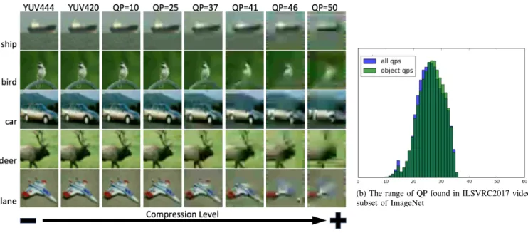
To consider the effects of compression in CNNs, we must first understand the mechanics of compression. Numerous standards are available for compression but MPEG-2 [20] and H.264/AVC [21] are the most widespread. A brief overview is given here but for futher details of H.264/AVC, the reader is referred to [21]–[23]. Figure 1a shows how H.264/AVC affects the tiny images of CIFAR-10.

All compression can be lossy or lossless. In most cases, video compression is lossy as the first stage in the process usually converts RGB data to YUV 4:2:0. This quarters

(a) The effects of quantisation on images from CIFAR-10

(b) The range of QP found in ILSVRC2017 video subset of ImageNet

Fig. 1. 1a There is no visual difference between YUV 4:4:4 and YUV 4:2:0 but the number of bytes used to represent the image has been reduced by half.

the colour resolution but halves the total number of bytes needed for storage and goes unnoticed by human eyes. JPEG compression can also apply this step. In general, CNNs trained on natural images learn distinctive edge-type Gabor filters and colour blobs in the first layer [24]. The use of YUV 4:2:0 in JPEG training images can explain this: colour blobs are lower resolution than intensity edges, just as the compressed colour component is of lower resolution than the intensity component. Another mechanism used in [21] removes redundancy by utilising existing data to make predictions and then encoding only the difference between actual data and predictions. Pre-diction is done at both frame level and block level. H.264/AVC commonly divides each frame into 16x16 pixel macroblocks for processing, which can cause blocking artifacts in more compressed video. An Intra (I or key) frame or block is constructed using only data within the same time interval. Intra frame compression can be applied directly to single images. As compression increases, blocks predicted from their neighbours become more like their neighbours and smooth colour transitions become banded. Inter (Predicted (P) or

Bidirectionally (B) predicted) frames use data from other frames in the bitstream, but ultimately refer back to I-frames. I-frames are the least compressed frame type, partly because there are fewer options for redundancy and partly because they are deliberately encoded with higher quality to provide a good quality reference for prediction.

Quantisation is the coarsest method of rate control in video compression and takes place in the frequency domain. Quantisation is expressed as:

C=round( δ

QP) (1)

Where C is the transmitted coefficient,δ is the frequency domain difference between prediction and actual and QP is

QuantisationParameter. A high QP yields a smaller bitstream

at the expense of more compression artifacts and lower quality. In H.264/AVC, the range of QP is 0 (lossless) to 52. Crucially, with a suitable rate control algorithm, QP varies both spatially and temporally throughout a video sequence. Thus an object’s visual quality can also vary spatially and temporally. Unlike natural changes in an object’s appearance, changes due to video compression quality may be measured objectively using data from the compressed bitstream.

This work examines both constant quality for reproducibility and constant bitrate for a real-world perspective. Figure 1b shows a normalised histogram of the spread of QP found in ILSVRC2017 bitstreams for complete frames and the areas within the defined bounding box of the first object in the sequence. There is little difference in QP between the subject of each video and the background, indicating that the encoder used to compress the sequences does not differentiate between the two. The average QP of all the frames is 25.52 and the average QP of the first object’s bounding boxes is 25.74. More interestingly, the I frames have average QP = 21.93, much lower than the sequence average. The same object will be compressed at different levels of quality in different frames. If a classifier is used to track objects over a sequence of frames, some objects may be missed due to changing compression levels in different frames. The data in Figure 1b, however, may reflect the ILSVRC2017 dataset itself rather than the real world.

A. Measuring image quality

For image quality assessment, we used both Peak Signal to Noise Ratio (PSNR) and Structural Similarity (SSIM) [25]. In video compression, it is common to utilise full reference quality metrics which directly compare uncompressed and compressed images to gain an objective metric. In images with a bit depth of 8, PSNR is calculated as:

(a) YUV (b) QP=10 (c) QP=25 (d) QP=37 (e) QP=50

Fig. 2. An example image from STL-10 when compressed at different compressions. Small block artifacts visible around the rigging of the ship diminish as the image is compressed but after QP=25, detail is lost.

P SN R= 20log10(√255

M SE) (2)

where MSE is the Mean Squared Error. PSNR does not account for the visual effect of neighbouring pixels. It is simply a measure of the difference between co-located pixels in the test and reference images.

The details of SSIM can be found in [25]. In short, SSIM has a range of 0-1 and endeavours to closely model human perception. It accounts for how the human visual system is affected by high frequency areas in images as well as contextual pixel intensity.

III. METHODS

The main motivation of this experiment is to explore how the quality of CNN training data determines performance on test data of the same or different quality. Because we examine the spatial effects of video compression in isolation and not the temporal effects, it is acceptable to use an image classifier. This also correlates with how CNN object classifiers are commonly used on individual frames of video. We selected a number of image datasets (MNIST [26], CIFAR-10 [2], labelled images of STL-CIFAR-10 [27]), to synthesise video-frame datasets. This avoids any pre-existing video compression artifacts that may be found in video datasets. Each of the synthesised datasets was then used individually to train a CNN. One CNN was trained using all the synthesised datasets together. Each trained CNN was then tested with all related test sets individually, to see whether features learned using one dataset were immediately transferable to another, closely related dataset.

For the purposes of this experiment, the images in CIFAR-10 were considered uncompressed. CIFAR-CIFAR-10 is based on a subset of Tiny Images [28] where original images were resized to 32x32 pixels. When the image resolution is reduced, so, too, are any spatial compression artifacts. JPEG compression com-monly uses an 8x8 block size, so any CIFAR-10 image with original dimensions over 256x256 pixels has blocking artifacts effectively removed. Banding artifacts are also comparatively reduced. To generate a series of uncompressed larger images, the CIFAR-10 dataset was resized to 64x64 (double height and width, Lanczos interpolation [29] for smoothing).

The basic set of experiments was also performed using MNIST. The single binary channel of MNIST was used as

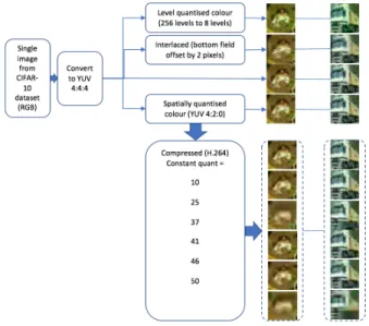
Fig. 3. Generation of constant quality datasets

the Y-channel in YUV data, with constant values of 128 for the U and V channels to give a greyscale image.

Finally, the labelled images only of STL-10 were used. The images are 96x96x3 and there are 13000 labelled images in the dataset. Prior to dataset synthesis, these were split into 80% training and 20% testing, ensuring an even split of class labels. Like CIFAR-10, this dataset is supplied as RGB pixel values, so there is no way to objectively quantify any previous compression, however compression artifacts can be seen when viewing some of the individual images (Figure 2) so these images were not considered uncompressed.

A. Dataset synthesis

Every training set and every test set (Table I) was synthe-sised using the same split of original images. This resulted in images across related datasets that were visually similar (Figure 1a) but no data leakage between test and train sets.

Interlaced frames were produced by offsetting every alter-nate row of YUV 4:4:4 by 2 pixels. Interlacing is a historical technique in broadcast video where the top field (odd rows) and the bottom field (even rows) are captured individually and is accounted for specifically in [21]. Interlacing produces vis-ible comb effects but enables further compression and general bitrate smoothing. Our simulation of interlacing mimics the comb effects of a slow camera pan over a static scene. In the

TABLE I

ASUMMARY OF SYNTHESISED DATASETS

Dataset Name Description

The following were applied to CIFAR-10, MNIST and STL-10

YUV 4:4:4 Lossless translation of RGB to YUV colour space

YUV 4:2:0 Lossless intensity (Y), colour (UV) at one quarter resolution, spatially averaged

Level UV Lossless intensity (Y), colour (UV) quantised to 8 uniformly spaced levels

Interlaced Offset alternate horizontal lines by 2 pixels

q(QP) f(F) Compressed frame number(F) = [0,2,3,6] with Quantisation Parameter(QP) = [10, 25, 37, 41, 46, 50];

The following were applied to CIFAR-10 only

q(QP) f(F) Compressed frame number(F) = [0,2,3,6] with bitrate(QP) >52

Fig. 4. The 7 frames of a short, synthesized video. The invariant image is overlaid onto a moving background of upwards scrolling horizontal lines. The background border adds 8 pixels on each side so that of the 9 macroblocks comprising the image, 8 contain moving data. This forces the compression codec to use predicted blocks with motion compensation, rather than skipped blocks as it would with a repeated image.

real world the extent of these effects depend on object motion relative to the camera.

The YUV 4:2:0 dataset was used to synthesise compressed video frame datasets (Figure 3). Still images were used to make a simple 7-frame video (Figure 4). This sequence was compressed using constant QP or bitrate, a Group Of Pictures (GOP) structure of IBBPBBP and one-pass encoding. Bitrates and quantisation parameters were manually selected to allow a range of quality in the video sequences. The extracted frames were of the frame types: Intra frame (0);Bi-directional frame (2);Predicted frame (3,6).

B. Network architecture

The network used in the experiments is conv5x5-64, pool3x3, conv5x5-64, pool3x3, fc-384, fc-192, softmax. ReLU was used. The learning rate was fixed at 0.1. This network is known to achieve a precision of around 84% on RGB CIFAR-10 after 30k iterations and approximately 86% after 60k iterations. The purpose of these experiments is not to directly enhance state-of-the-art but to investigate the effects of video compression on learning. Frames derived from CIFAR-10 were normalised by subtracting the average pixel value from all pixels. For data augmentation, the images were randomly cropped from 32x32 to 28x28 and randomly horizontally flipped during training. The test set was centrally cropped and normalised. MNIST frames were normalised but no further augmentation. STL-10 derived frames were normalised and flipped only.

It was found that switching from RGB24 colour space to YUV 4:4:4 had no impact on precision, as intuitively expected.

C. Training and testing

A model was trained on every dataset in the series and each model was tested with every related dataset (Table II) and the

mean Average Precision (mAP) recorded.

To examine the effect of pre-training, a CNN was ini-tialised with all the weights and biases learned on one synthesised dataset and allowed to further train on another. Specifically:

• pre-trained on uncompressed YUV4:4:4, further trained

on uncompressed YUV4:4:4

• pre-trained on uncompressed YUV4:4:4, further trained on highly compressed QP 50

• pre-trained on highly compressed QP 50, further trained on uncompressed YUV4:4:4

• pre-trained on highly compressed QP 50, further trained on highly compressed QP 50

IV. RESULTS AND DISCUSSION

One of the main findings is that CNNs respond to com-pressed video in an intuitive way. In general, more comcom-pressed video leads to lower classification precision (Figure 7, Table III). The effects of heavy compression distort objects enough to render them unrecognisable by human eyes (Figure 1a), and the results (Figure 7) show that this is broadly matched in machine vision. The maximum precision for a given test set is generally achieved by a network trained with data most similar to that of the test set. A network trained with a variety of different compression levels becomes a ”jack of all trades, master of none” (Table III).

Features learned on one compression level transfer well to less compressed video: a network trained on video frames compressed with a particular QP achieves at least the same precision on frames compressed with a lower QP. Similarly, a network trained on video frames compressed at a given bitrate performs equally well or better when tested with frames compressed at a higher bitrate. Conversely, although a network trained on high quality frames achieves better precision when tested with frames of high quality, it experiences greater drop off in precision when faced with lower quality data.

A. Colour spaces

In datasets with no video compression (YUV 4:4:4, YUV 4:2:0, level UV and interlaced), features trained oninterlaced

frames do not transfer well to non-interlaced frames (Table IV). Moreover, networks trained on non-interlaced data did not achieve good precision on interlaced test data. Features learned on interlaced data were more transferable to non-interlaced

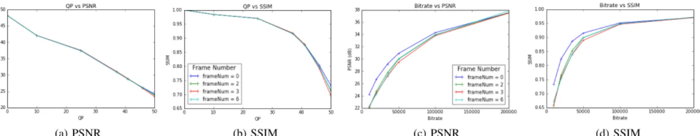
(a) PSNR (b) SSIM (c) PSNR (d) SSIM

Fig. 5. The effects of constant quantisation and rate control on image quality metrics (CIFAR-10). Different frame types produce very similar graphs, except for Intra frames with rate control which are higher quality than the others.

TABLE II RELATED DATASETS

Source dataset Synthesised (related) datasets

CIFAR-10 YUV 4:4:4, YUV 4:2:0, Level UV, Interlaced, q(QP) f(F);(QP) = [10, 25, 37, 41, 46, 50];(F) = [0,2,3,6]

CIFAR-10 YUV 4:4:4, YUV 4:2:0, Level UV, Interlaced, q(QP) f(F); QP>52;(F) = [0,2,3,6]

CIFAR-10-double YUV 4:4:4, YUV 4:2:0, Level UV, Interlaced, q(QP) f(F);(QP) = [10, 25, 37, 41, 46, 50];(F) = [0,2,3,6]

MNIST YUV 4:4:4, YUV 4:2:0, Level UV, Interlaced, q(QP) f(F);(QP) = [10, 25, 37, 41, 46, 50];(F) = [0,2,3,6]

STL-10 YUV 4:4:4, YUV 4:2:0, Level UV, Interlaced, q(QP) f(F);(QP) = [10, 25, 37, 41, 46, 50];(F) = [0,2,3,6]

(a) YUV (b) QP=10 (c) QP=37 (d) QP=50 (e) Double (f) interlaced Fig. 6. The first layer filters, constant QP training on CIFAR-10 (re-ordered according to variance in each filter)

TABLE III

MEANAVERAGEPRECISION FOR NETWORKS CROSS EVALUATION ON CIFAR-10INTRA FRAME. BEST TRAINED NETWORK FOR THIS TEST UNDERLINED; BEST TEST RESULT FOR THIS TRAINED NETWORK INBOLD.

Trained On (QP) Tested With (QP) All YUV 10 25 37 41 46 50 YUV 73.6 84.0 83.4 82.6 78.8 75.0 67.7 60.9 10 73.7 83.6 83.5 82.6 79.3 75.1 68.1 61.0 25 73.5 82.1 82.5 82.2 79.0 75.4 68.0 61.0 37 70.6 73.1 73.5 74.6 76.9 74.4 68.8 61.0 41 67.6 63.6 63.5 65.7 71.4 72.3 67.9 61.6 46 60.1 48.4 48.0 49.7 58.2 62.3 64.2 59.9 50 53.3 36.1 36.7 37.7 44.4 50.3 57.0 57.9

data than vice versa. Visualisation of the filters learned in the first layer of the CNN (Figure 6) shows some combing effects. It can be theorised that features from CNNs trained only on still image data or photographs which do not contain interlaced data will perform less well on interlaced videos. This effect diminished with a larger frame size (Table IV), so smaller features may be more affected by interlacing, but further research is needed to confirm this. It is common to resize video and images for neural networks [10], [30], and this reduces combing effects. A de-interlacing filter may be

TABLE IV

MEANAVERAGEPRECISION FOR NETWORKS TRAINED/TESTED ON DIFFERENT UNCOMPRESSED COLOUR SPACES GENERATED FROM

CIFAR-10 [SINGLE IMAGE DIM;DOUBLE IMAGE DIM] Trained On Tested With YUV 4:4:4 Level UV YUV 4:2:0 Interlaced YUV 4:4:4 84.0; 82.0 83.4; 81.1 83.4; 81.8 59.3; 53.8 Level UV 83.3; 80.1 83.6; 81.2 82.8; 80.2 57.9; 53.3 YUV 4:2:0 83.7; 81.8 83.2; 80.7 83.4; 81.5 58.2; 53.0 Interlaced 37.3; 78.2 39.8; 76.5 33.0; 78.2 82.0; 81.6

applied but this will cause some blurring. Although this is not examined here, we hypothesise that de-interlacing artifacts will reduce CNN performance.

Decreased colour information, either by quantisation to fixed levels or by reduction of colour resolution, does not have a large impact on maximum achievable precision (Table IV). A drop in colour data in the training set or the test set leads to a drop in mean average precision, however reducing colour resolution to one quarter of its original value (as in YUV 4:4:4 to YUV 4:2:0 conversion) does not significantly impact classification (mAP difference of 0.6%). This may be partly attributed to the shape of the learned filters: it is possible that the most discriminative filters, like human eyes, weight

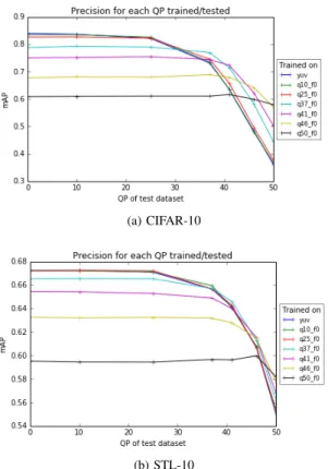
(a) CIFAR-10

(b) STL-10

Fig. 7. Features learned on a given QP transfer well to test data encoded with the same QP or lower, best viewed in colour

luma (intensity) more strongly than chroma (colour).

B. Constant quality

The maximum achievable mAP generally reduces as quan-tisation of the training data increases. Interestingly, the maxi-mum mAP for each network does not necessarily coincide with testing on its related dataset (Table III). The network trained on data with QP=50, for example, gives its lowest mAP when tested with QP=50 data. In general, slightly higher precision is achieved when a network is tested with data of a lower QP than than of its training set. Conversely, test data with a specific QP achieves the best precision when passed through a network trained on a similar QP.

The plots of the networks trained on STL-10 are very close together for uncompressed, QP=10 and QP=25 (Figure 7). Us-ing a modified network architecture with an additional conv5-64 layer, networks trained on QP=10 and QP=25 outperformed those trained on uncompressed data. This can be explained by visible compression artifacts in the original image Figure 2). Some uncompressed images show blocking artifacts that are visibly reduced by compressing with QP=10, and still further reduced with QP=25. This is a serendipitous effect of compression. At QP=37 and above, introduced compression artifacts come into play and the maximum mAP is conse-quently reduced.

The first layer filters of a neural network are known to give an indication of the low level features learned in the network. An examination of these for the network trained on

CIFAR-10 data (Figure 6) shows that networks trained on higher QP data rely more heavily on colour-based filters rather than intensity filters. Intensity filters learned on high QP data are far less distinct than their low QP counterparts. This corresponds with the idea that the effects of quantisation in the frequency domain manifest visually as blurring.

It was found that MNIST data was very robust against video compression. Video compression applied to MNIST gave a range of SSIM from 0.74 and PSNR from 21.0 dB. Application of constant quality compression to CIFAR-10, yielded minimum SSIM = 0.36 and PSNR = 16.9 dB. For STL-10: minimum SSIM = 0.42 and PSNR = 19.41 dB. While PSNR gives an indication of how the compressed signal differs from the original, SSIM gives a better indication of visual

difference. The networks trained on datasets synthesised from MNIST showed little change in performance when tested with data of a different compression level. The pattern of increasing QP leading to decreasing mAP was still present, however the mAP ranged from 97.0% to 99.2% for non-interlaced data. and 95.0% to 99.3% for interlaced data.

The range of SSIM shows how compression affects the data. The smaller range of quality metrics for compressed datasets synthesised from STL-10 shows that CIFAR-10 is more adversely affected by compression and this relates to the range of mAP (Figure 7). Datasets derived from STL-10 have a lower range of SSIMandmAP than those derived from CIFAR-10.

C. Frame type

When using constant QP, frame-type (I, B, P) has little effect on CNN classification, with average variation of 0.6% mAP, and slightly better performance for networks trained on frame 0. This ties in with the quality metrics shown in Figures 5a and 5b where it can be seen that, with constant QP, there is very little difference between the frame types. For constant bitrate, this effect was more marked, with an average range of 1% mAP and networks trained on frame 0 exhibiting higher performance. Similarly, testing with I-frames also achieves higher performance than P- or B-frame test batches. This can be attributed to rate control mechanisms in x264 which allocate more bits to I-frames, and thus a lower average QP as illustrated in Figures 5c and 5d.

D. Constant Bitrate

The graph of networks trained on datasets of different target bitrates (Figure 8) shows similar results to those for constant QP: more compressed data yields lower achievable mAP, but networks trained solely on uncompressed or high bitrate data perform poorly when classifying low bitrate frames.

E. Double Image Dimensions

For double image dimensions, results were broadly similar to those found above: networks trained on uncompressed data achieve the highest mAP of 82% but this drops off most quickly when tested with lower quality data. Networks trained on lower quality data achieved lower maximum mAP

Fig. 8. Features learned on a given bitrate transfer well to test data encoded with the same bitrate or higher

and produced equal or better mAP when tested with higher quality data. Most interestingly, Table IV shows that the drop in performance for interlaced data was much lower in this experiment. This can be attributed to the network learning spatially larger discriminative features (Figure 6) and also because the interlaced offset was maintained as 2 pixels so the combing effect was proportionately smaller on larger im-ages. A further experiment was performed using the network architecture with an extra conv5-64 layer. The results showed improved performance ( 7% absolute mAP) of the interlaced-data-trained network when tested with non-interlaced data. This suggests that deeper layers may effect some form of deinterlacing but further research is needed.

Another intuitive result is in the visualisation of the first layer filters (Figure 6): doubling the image dimensions of the dataset without changing the kernel size of the first layer sim-ply doubles the learnt feature size. This is significant because it helps explain the common appearance of first layer filters trained on natural images. If training images utilise YUV 4:2:0 colour space, then chroma resolution is one quarter of luma resolution. Therefore, colour features learned in CNNs are also lower resolution than their intensity (edge-type) counterparts. This implies that the use of YUV 4:2:0 is widespread in JPEG data used to train many modern networks. Hypothetically, the first layer features of a network trained on YUV 4:4:4 data would exhibit colour-edge features rather than colour blobs.

F. Pretraining

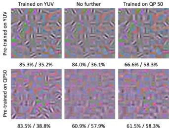
The results for pre-training (Figure 9) show a network can be fine tuned towards different levels of compression but this reduces precision for the original data. In the case of a network pre-trained on uncompressed data (Figure 9, top row), the differences in the first layer filters are very slight but the differences in mAP are marked. This suggests that much of the fine tuning is achieved in higher layers of the network which. For the network pre-trained on uncompressed data and further trained on highly compressed data (Figure 9, top right), the edge-type filters in the first layer do not visually blur. It can be hypothesised that the increase in mAP from 36.1% to 58.3% comes from the equivalent of feature blurring in deeper

Fig. 9. The filters learned in the first layer with pre-training: the central column shows the original trained network with no further training, the left column has been further trained with uncompressed data, the right column has been further trained with the most compressed data [mAP on uncompressed / QP 50 data]

layers. Sharp features in the first layer are required for mAP on uncompressed data.

Pre-training a network with QP = 50 and further training with uncompressed data (Figure 9, bottom left), allows sharp edge-type filters to emerge in the first layer and the mAP for uncompressed data improves, at the expense of highly compressed data. Further training with compressed data might allow deeper layers of the network to generalise around these sharp features and improve compressed test precision. The mAP improves on both compressed and uncompressed test sets when the network is further trained on highly compressed data (Figure 9, bottom right). This improvement is small but follows the trend shown in Figure 7 where features learned on compressed data transfer successfully to less compressed datasets.

G. Limitations

We synthesise our own video datasets from still images for these experiments. Intra frame compression can be validly performed on single frames, and the results here focus on the first intra frame of the sequence. In compressing artificially constructed video sequences, video encoders may make un-naturally constrained compression decisions, so the effects of

frame typemay be understated in these experiments. V. CONCLUSIONS

With high prevalence of compressed video and increasing use of CNNs for video analysis, we have provided a timely evaluation of the effects of video compression on classification by CNNs. We found that the highest precision on a given test set occurs when the network is trained on a similarly compressed dataset. Features learned in networks trained on highly compressed frames are equally valid when testing less compressed data, but the precision of the network is

generally lower than that of one trained on uncompressed frames. A network trained on images of a specific quality disproportionately misclassifies objects of a worse quality but mostly maintains performance when classifying data of a similar or better quality. Networks trained on highly quantised video frames learn more colour features in their first layer than networks trained on high quality frames which learn more edge-type features. First layer colour features perform better than edge features for classifying low quality frames, but it is possible for higher layers to compensate for this when a network has been pretrained on uncompressed data. A network trained on a variety of levels of compression achieves lower precision than specialised networks, so using different levels of compression as a form of data augmentation will not improve performance on all data.

We also explain how the use of compressed YUV 4:2:0 shapes the first layer filters of CNNs trained on natural images. Lower colour resolution in training data means the filters diverge into higher resolution edge-type filters and lower resolution colour blobs. Higher resolution colour features may emerge from CNNs trained on uncompressed images.

A. Future Work

This study has looked only at a small subsection of image classification and compression, but further work is necessary to ascertain whether the patterns observed here are present in deeper networks and how they can be applied to improve video classification or identification and localisation of objects within videos.

The work here suggests that information about a compressed video bitstream, such as quantisation, can inform models for classification and video analysis and improve performance. Our future work will examine how this information can be deduced directly from the pixels for multiply compressed videos.

REFERENCES

[1] J. Deng, W. Dong, R. Socher, L.-J. Li, K. Li, and L. Fei-Fei, “Imagenet: A large-scale hierarchical image database,” in Computer Vision and Pattern Recognition, 2009. CVPR 2009. IEEE Conference on. IEEE, 2009, pp. 248–255.

[2] A. Krizhevsky and G. Hinton, “Learning multiple layers of features from tiny images,” 2009.

[3] K. He, X. Zhang, S. Ren, and J. Sun, “Delving deep into rectifiers: Surpassing human-level performance on imagenet classification,” in Proceedings of the IEEE international conference on computer vision, 2015, pp. 1026–1034.

[4] S. Abu-El-Haija, N. Kothari, J. Lee, P. Natsev, G. Toderici, B. Varadara-jan, and S. Vijayanarasimhan, “Youtube-8m: A large-scale video classi-fication benchmark,”arXiv preprint arXiv:1609.08675, 2016. [5] A. Karpathy, G. Toderici, S. Shetty, T. Leung, R. Sukthankar, and

L. Fei-Fei, “Large-scale video classification with convolutional neural networks,” inCVPR, 2014.

[6] O. Russakovsky, J. Deng, H. Su, J. Krause, S. Satheesh, S. Ma, Z. Huang, A. Karpathy, A. Khosla, M. Bernsteinet al., “Imagenet large scale visual recognition challenge,”International Journal of Computer Vision, vol. 115, no. 3, pp. 211–252, 2015.

[7] M. Kristan, J. Matas, A. Leonardis, T. Voj´ıˇr, R. Pflugfelder, G. Fer-nandez, G. Nebehay, F. Porikli, and L. ˇCehovin, “A novel performance evaluation methodology for single-target trackers,” IEEE transactions on pattern analysis and machine intelligence, vol. 38, no. 11, pp. 2137– 2155, 2016.

[8] Y. Wu, J. Lim, and M. H. Yang, “Online object tracking: A benchmark,” in Computer Vision and Pattern Recognition (CVPR), 2013 IEEE Conference on, June 2013, pp. 2411–2418.

[9] K. Simonyan and A. Zisserman, “Very deep convolutional networks for large-scale image recognition,” arXiv preprint, vol. arXiv:1409.1556, 2014.

[10] A. Krizhevsky, I. Sutskever, and G. E. Hinton, “Imagenet classification with deep convolutional neural networks,” inAdvances in neural infor-mation processing systems, 2012, pp. 1097–1105.

[11] M. Danelljan, G. Hager, F. Shahbaz Khan, and M. Felsberg, “Con-volutional features for correlation filter based visual tracking,” in The IEEE International Conference on Computer Vision (ICCV) Workshops, December 2015.

[12] M. Danelljan, A. Robinson, F. S. Khan, and M. Felsberg, “Beyond correlation filters: Learning continuous convolution operators for visual tracking,” inEuropean Conference on Computer Vision. Springer, 2016, pp. 472–488.

[13] C. Ma, J.-B. Huang, X. Yang, and M.-H. Yang, “Hierarchical con-volutional features for visual tracking,” in The IEEE International Conference on Computer Vision (ICCV), December 2015.

[14] L. Wang, W. Ouyang, X. Wang, and H. Lu, “Visual tracking with fully convolutional networks,” in The IEEE International Conference on Computer Vision (ICCV), December 2015.

[15] P. Zhang, T. Zhuo, W. Huang, K. Chen, and M. Kankanhalli, “Online object tracking based on CNN with spatial-temporal saliency guided sampling,”Neurocomputing, 2017.

[16] H. Liu, Q. Zheng, M. Luo, D. Zhang, X. Chang, and C. Deng, “How unlabeled web videos help complex event detection?” 2017.

[17] Z. Zhao, Q. Yang, D. Cai, X. He, and Y. Zhuang, “Video question answering via hierarchical spatio-temporal attention networks,” in In-ternational Joint Conference on Artificial Intelligence (IJCAI), vol. 2, 2017.

[18] J. Yue-Hei Ng, M. Hausknecht, S. Vijayanarasimhan, O. Vinyals, R. Monga, and G. Toderici, “Beyond short snippets: Deep networks for video classification,” inProceedings of the IEEE conference on computer vision and pattern recognition, 2015, pp. 4694–4702.

[19] S. Dodge and L. Karam, “Understanding how image quality affects deep neural networks,” inQuality of Multimedia Experience (QoMEX), 2016 Eighth International Conference on. IEEE, 2016, pp. 1–6.

[20] ITU-T, H.262 Information technology - Generic coding of moving pictures and associated audio information: Video, ITU-T, 2 2012. [21] ——,H.264 Advanced video coding for generic audiovisual services,

ITU-T, 10 2016.

[22] I. E. Richardson, The H. 264 advanced video compression standard. John Wiley & Sons, 2011.

[23] T. Wiegand, G. J. Sullivan, G. Bjontegaard, and A. Luthra, “Overview of the h.264/avc video coding standard,”IEEE Transactions on Circuits and Systems for Video Technology, vol. 13, no. 7, pp. 560–576, July 2003.

[24] J. Yosinski, J. Clune, Y. Bengio, and H. Lipson, “How transferable are features in deep neural networks?” inAdvances in neural information processing systems, 2014, pp. 3320–3328.

[25] Z. Wang, A. C. Bovik, H. R. Sheikh, and E. P. Simoncelli, “Image quality assessment: from error visibility to structural similarity,”IEEE transactions on image processing, vol. 13, no. 4, pp. 600–612, 2004. [26] Y. LeCun, C. Cortes, and C. J. Burges, “The mnist database of

handwritten digits,” 1998.

[27] A. Coates, A. Ng, and H. Lee, “An analysis of single-layer networks in unsupervised feature learning,” in Proceedings of the fourteenth international conference on artificial intelligence and statistics, 2011, pp. 215–223.

[28] A. Torralba, R. Fergus, and W. T. Freeman, “80 million tiny images: A large data set for nonparametric object and scene recognition,” IEEE transactions on pattern analysis and machine intelligence, vol. 30, no. 11, pp. 1958–1970, 2008.

[29] K. Turkowski, “Turkowski filters for common resampling tasks,” 1990. [30] J. Redmon, S. K. Divvala, R. B. Girshick, and A. Farhadi, “You only look once: Unified, real-time object detection,” CoRR, vol. abs/1506.02640, 2015. [Online]. Available: http://arxiv.org/abs/1506.02640