DISSERTATION
Defence held on 09/01/2020 in Esch-sur-Alzette to obtain the degree of
DOCTEUR DE L’UNIVERSITÉ DU LUXEMBOURG
EN INFORMATIQUE
by
Sasan JAFARNEJAD
Born on 14 December 1988 in Tehran (Iran)M
ACHINE
L
EARNING
-
BASED
M
ETHODS FOR
D
RIVER
I
DENTIFICATION AND
B
EHAVIOR
A
SSESSMENT
: A
PPLICATIONS FOR
CAN
AND
F
LOATING
C
AR
D
ATA
Dissertation defence committee
Dr. Thomas Engel, dissertation supervisorProfessor, Université du Luxembourg
Dr. German Castignani, Vice Chairman
Motion-S
Dr. Johan Wahlström
Researcher, Oxford University
Dr. Francesco Viti, Chairman
Associate professor, Université du Luxembourg
Dr. Marco Fiore
yourself.”
The exponential growth of car generated data, the increased connectivity, and the advances in artificial intelligence (AI), enable novel mobility applications. This dis-sertation focuses on two use-cases of driving data, namely distraction detection and driver identification (ID). Low and medium-income countries account for 93% of traffic deaths [1]; moreover, a major contributing factor to road crashes is distracted driv-ing [2]. Motivated by this, the first part of this thesis explores the possibility of an easy-to-deploy solution to distracted driving detection. Most of the related work uses sophisticated sensors or cameras, which raises privacy concerns and increases the cost. Therefore a machine learning (ML) approach is proposed that only uses signals from the CAN-bus and the inertial measurement unit (IMU). It is then evaluated against a hand-annotated dataset of 13 drivers and delivers reasonable accuracy. This approach is limited in detecting short-term distractions but demonstrates that a viable solution is possible. In the second part, the focus is on the effective identification of drivers using their driving behavior. The aim is to address the shortcomings of the state-of-the-art methods. First, a driver ID mechanism based on discriminative classifiers is used to find a set of suitable signals and features. It uses five signals from the CAN-bus, with hand-engineered features, which is an improvement from current state-of-the-art that mainly focused on external sensors. The second approach is based on Gaussian mixture models (GMMs), although it uses two signals and fewer features, it shows improved accuracy. In this system, the enrollment of a new driver does not require retraining of the models, which was a limitation in the previous approach. In order to reduce the amount of train-ing data a Triplet network is used to train a deep neural network (DNN) that learns to discriminate drivers. The training of the DNN does not require any driving data from the target set of drivers. The DNN encodes pieces of driving data to an embedding space so that in this space examples of the same driver will appear closer to each other and far from examples of other drivers. This technique reduces the amount of data needed for accurate prediction to under a minute of driving data. These three solutions are validated against a real-world dataset of 57 drivers. Lastly, the possibility of a driver ID system is explored that only uses floating car data (FCD), in particular, GPS data from smartphones. A DNN architecture is then designed that encodes the routes, origin, and destination coordinates as well as various other features computed based on contextual information. The proposed model is then evaluated against a dataset of 678 drivers and shows high accuracy. In a nutshell, this work demonstrates that proper driver ID is achievable. The constraints imposed by the use-case and data availability negatively affect the performance; in such cases, the efficient use of the available data is crucial.
This work was conducted at the SECAN-Lab of the University of Luxembourg’s Interdisciplinary Centre for Security Reliability and Trust (SnT).
First and foremost, I would like to thank Prof. Dr. Thomas Engel for allowing me to conduct my research at SECAN-Lab and letting me explore and investigate my topics of interest freely. Second, I would like to thank Dr.-Ing. German Castignani, for his invaluable guidance, support, encouragement, and the much-needed criticism of my research. Third, I would like to thank Dr. Fabian Lanze for his constructive feedback on my work.
I want to thank my friends and the former members of the VehicularLab, especially Walter, Thierry, Lara, and my former office mates, Salvatore, Chris, and Mathis. I also thank all my colleagues at SECAN-Lab and SnT, who have been part of this journey and made the work enjoyable.
I express my deepest gratitude to my long-time friends, Hossein and Sam, for their unconditional support throughout the past four years.
Most of all, I would like to thank my family, especially my mom Robabeh, my sister Raheleh, my brothers Mohammad and Abbas, and Samira, for always supporting me and encouraging me with their best wishes.
The experiments presented in this dissertation were carried out using the HPC facilities of the University of Luxembourg [3]. Moreover, this work would not be pos-sible without the datasets kindly provided by Motion-S S.A. and VPALAB of Sabanci University.
Abstract ii
Acknowledgements iii
List of Figures viii
List of Tables x 1 Introduction 1 1.1 Research Question . . . 3 1.2 Methodology . . . 4 1.3 Contributions . . . 5 1.4 Manuscript Structure . . . 6 2 Uyanik Dataset 8 2.1 Parsing Data . . . 10
2.2 Sample-rate and Synchronization . . . 10
2.3 Data Quality . . . 10
2.4 Exploratory Data Analysis . . . 11
I Distracted Driving Detection 16 3 Introduction to Distracted Driving Detection 17 3.1 State-of-the-art . . . 18
4 Non-Intrusive Distracted Driving Detection Based on Driving Data 21 4.1 Methodology . . . 22
4.1.1 Evaluation Method . . . 22
4.2 Video Annotation and Synchronization with Sensors . . . 23
4.2.1 Feature Extraction . . . 24 4.2.2 Feature Importance . . . 25 4.2.3 Classification Algorithms . . . 26 4.2.4 Decision Functions . . . 27 4.3 Model Performance . . . 27 4.3.1 Frame-size Analysis . . . 27 4.3.2 Classifier Benchmarks . . . 28 iv
4.3.3 Decision Function Benchmarks . . . 29
4.4 Discussion . . . 30
4.5 Summary . . . 31
II Driver Identification 33 5 Introduction to Driver Identification 34 5.1 Applications of Driver Identification . . . 36
5.2 Driver Identification as a Privacy Issue . . . 38
5.2.1 Threat Model . . . 39
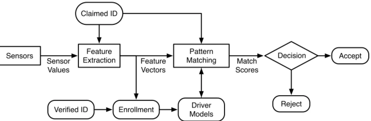
5.3 Elements of a Driver Identification System . . . 39
5.4 Design Constraints . . . 40
5.4.1 Communication and Computation . . . 40
5.4.2 Data Availability . . . 40
5.4.3 Use-case Requirements . . . 41
5.5 State-of-the-art . . . 41
5.5.1 Taxonomy of Related Work . . . 41
5.5.2 Most Relevant Studies . . . 42
5.6 What To Expect From The Following Chapters? . . . 46
6 Driver Identification Using Discriminative Classifiers 48 6.1 Methodology . . . 49
6.1.1 Preprocessing and Feature Extraction . . . 51
6.1.2 Classification Algorithms . . . 54
6.1.3 Decision Functions . . . 55
6.2 Feature Analysis . . . 56
6.2.1 Statistical Features . . . 56
6.2.2 Cepstral and Spectral Features . . . 58
6.2.3 Overall Feature Importance . . . 59
6.2.4 Frame-size Analysis . . . 60
6.3 Experiments . . . 61
6.3.1 Classifier Benchmarks . . . 61
6.3.2 Decision Functions . . . 62
6.3.3 Sensitivity Analysis of Training-data . . . 62
6.3.4 Sensitivity Analysis of Decision Window . . . 63
6.3.5 Real-time Identification . . . 64
6.4 Discussion . . . 64
6.5 Summary . . . 65
7 Driver Identification using Gaussian Mixtures 67 7.1 Methodology . . . 68
7.1.1 The Gaussian Mixture Driver Model . . . 68
7.1.2 Driver Identification . . . 69
7.1.3 Model Fusion . . . 69
7.1.4 Evaluation Method . . . 70
7.1.5 Feature Extraction . . . 71
7.3 Experiments . . . 72
7.3.1 Model Parameters . . . 72
7.3.2 Sensitivity Analysis of Training-data . . . 74
7.3.3 Sensitivity Analysis of Decision Window . . . 75
7.3.4 Overall Identification Performance . . . 75
7.4 Discussion . . . 75
7.5 Summary . . . 76
8 Driver Embedding and Its Applications to Driver Identification 78 8.1 Methodology . . . 79
8.1.1 Deep Driver Model . . . 79
8.1.2 Training . . . 81 8.1.3 Input Data . . . 82 8.1.4 Embedding Network . . . 83 8.2 Evaluation . . . 84 8.2.1 Experimental Setup . . . 84 8.3 Experiments . . . 85 8.3.1 Driver Identification . . . 85 8.3.2 Driver Verification . . . 87 8.4 Embedding Visualization . . . 88 8.5 Discussion . . . 90 8.6 Summary . . . 91
9 Driver Identification Using GPS Data from Smartphone 92 9.1 Dataset . . . 93
9.1.1 Preprocessing . . . 94
9.1.2 Features . . . 95
9.1.2.1 Semantic Categorization of Features . . . 95
9.1.2.2 Technical Categorization of Features . . . 96
9.2 Methodology . . . 97
9.2.1 Neural Network Architecture . . . 98
9.3 Experimental Setup . . . 100 9.3.1 Hyperparameter Search . . . 101 9.3.2 Baseline Algorithms . . . 101 9.3.2.1 LightGBM . . . 101 9.3.2.2 HMM-based Model . . . 102 9.3.2.3 Combined Model . . . 102 9.4 Experimental Results . . . 103
9.4.1 Comparison with Baselines . . . 103
9.4.2 Semantic Feature Categories . . . 104
9.4.3 Effectiveness of Cross-features . . . 106
9.4.4 Sensitivity Analysis of Training-data . . . 107
9.5 Discussion . . . 107
9.6 Summary . . . 108
10 Conclusion 110 10.1 Summary of Contributions . . . 111
10.1.1 Distracted Driving Detection . . . 111
10.1.2 Driver Identification . . . 111
10.2 Final Discussion . . . 113
10.2.1 Privacy Considerations . . . 115
10.3 Future Research Perspectives . . . 116
Abbreviations 118
2.1 Trip lengths in the Uyanik dataset . . . 12
2.2 A trip from the Uyanik dataset . . . 13
2.3 Histogram of main signals for all drivers in Uyanik dataset . . . 13
2.4 Histogram of driving signals for 5 drivers . . . 14
2.5 An example snapshot of raw sensor data . . . 15
4.1 Distraction Detection Process . . . 22
4.2 Effect of Frame-size on Classification Score . . . 28
4.3 Estimator Performance Comparison . . . 28
4.4 Estimator Performance Comparison - Variable Frame-sizes . . . 29
5.1 Generic driver verification system. . . 39
6.1 Block Diagram of the Driver ID method . . . 49
6.2 Cross-validation scheme . . . 50
6.3 Feature extraction block diagram. . . 51
6.4 Visualization of Spectral and Cepstral Features . . . 53
6.5 Computation of Spectral and Cepstral Features . . . 53
6.6 Feature importances for statistical features . . . 57
6.7 Feature importance of statistical features per signal . . . 57
6.8 frame-size peformance evaluation . . . 58
6.9 Feature importance for 3 different frame-lengths of 2, 5, and 15 seconds. . 59
6.10 frame-size performance evaluation . . . 60
6.11 Classifier Identification Performance Comparison . . . 61
6.12 Influence of amount of training and prediction data on accuracy . . . 63
6.13 Prediction over time . . . 63
7.1 Method Architecture . . . 68
7.2 Feature Extraction Process . . . 71
7.3 Feature importance of spectral and cepstral features and their ∆&∆∆ . 72 7.4 GMM Parameters . . . 73
7.5 The impact of α on accuracy . . . 74
7.6 Identification Performance for GMM Approach . . . 74
8.1 Block diagram of Triplet network . . . 80
8.2 Simple visualization of Triplet loss . . . 81
8.3 A building block of residual learning . . . 83
8.4 1-dimensional ResNet . . . 84
8.5 Deep Driver model, Driver ID Performacne . . . 86
8.6 Deep driver model driver verification - EER . . . 87 viii
8.7 Visualization of embeddings for 4 experiments. . . 89
9.1 MS-Dataset data model . . . 93
9.2 MS-Dataset statistics . . . 94
9.3 Location cross-feature . . . 96
9.4 Architecture diagram . . . 97
9.5 Algorithm error-rate plot . . . 104
9.6 Error-rate per feature-set . . . 105
9.7 Top 20 most important features obtained from LightGBM . . . 106
2.1 Sensor Data Available in Uyanik . . . 9
4.1 Selected Signals for Driver Distraction Detection . . . 24
4.2 Average Scores For Each Signal . . . 25
4.3 Average Scores For Each Function . . . 26
4.4 Decision Function Performance - Results are for k-NN as classifier . . . 29
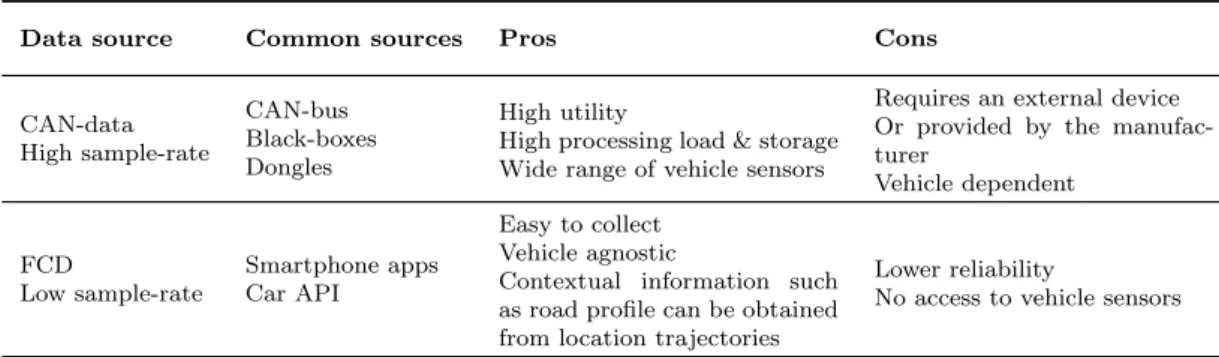
5.1 Driving data sources and their merits . . . 35
5.2 Summary of Driver Identification Literature . . . 43
6.1 Selected Signals for Driver Identification . . . 51
6.2 Comparison of decision functions . . . 62
6.3 Summary of the results . . . 65
7.1 Comparison of with previous approach . . . 76
9.1 Dataset statistics . . . 94
9.2 Metrics, and dimension of their corresponding feature vectors. . . 95
9.3 Summary of Model Parameters . . . 98
9.4 Hyper parameters of the model . . . 101
9.5 Effectiveness of location cross-features . . . 105
Richard Hamming
1
Introduction
The number of road deaths has reached 1.35 million per year in 2016 and continues to climb. It is the leading cause of death among children and young adults aged 5– 29 [1]. Last year in Europe, over 25,000 lost their lives in road collisions; in the United States, that number was over 40,000. European Union (EU) is committed to Vision Zero, a multi-national road safety project aimed to achieve a road traffic system with no fatalities [4]. European Union (EU) aims to reduce road death to almost zero by 2050. Although the EU’s preventive actions resulted in a 21% decrease between 2010 and 2018, this decrease has stagnated, and European countries missed their interim targets for the 2011–20 period [5]. For instance, in the United Kingdom, distraction or impairment was a contributory factor to 24% of fatal accidents in 2014, which has grown to 27% in 2017 [2]. A recent study shows that drivers use their phones in about 88% of their journeys [6]. Mobile phone increases the likelihood of a crash by fourfold [7]. Another critical contributory factor to fatal crashes is drowsy/fatigued driving. Fatigued driving increases the risk of involvement in crash or near-crash by nearly four times [8, 9]. Sleep deprivation can increase the risk of a crash by eight times [10], this should not come as a surprise since even moderate sleep deprivation impairs cognitive and motor performance,
equivalent to legally prescribed levels of alcohol intoxication [11]. Is it possible to detect
distracted driving using a system that is affordable and easy to deploy?
Drowsiness and fatigue are especially common among commercial long-haul drivers. Sleepiness/fatigue increases the involvement likelihood of a commercial vehicle in a fatal collision [12]. Many countries have put forward regulations to prevent long-haul truck
drivers from overwork. In Europe, the regulation (EC) No 561/2006 [13] defines driving
time and rest periods, and it is enforced using analog and smart tachographs introduced
by directive 165/2014 [14]. Meanwhile, a poll conducted by a union uncovers that in the month before the poll, 40% of drivers had been asked to exceed their duty hours, this is even worse among self-employed drivers [15]. Another study finds that over 70% of drivers work more than 11 hours daily, and 43% indicated that “sometimes to always” violate the working hours [16]. These drivers not only risk their own lives; they also endanger other road users. There are also indications that drivers tamper with these tachographs [17]. Is there a tamper-resistant way of enforcing these regulations? Perhaps tachographs that can recognize the drivers based on their driving style.
Ride-sharing applications such as Uber, Lyft, Bolt, have revolutionized transporta-tion by providing a level of comfort that once deemed unimaginable, but they have issues of their own. There have been many reports of sexual assault and various other crimes by ride-sharing drivers [18]. Drivers commit fraud or cheat the system by creating fake global positioning system (GPS) traces, initiating ride requests from stolen accounts, and more [19]. Introduction of background checks by the ride-sharing companies—now mandatory in some jurisdictions—has reduced the crime rates, but new workarounds emerge. Some drivers use stolen accounts or share the same account, which enables a myriad of problems. Similar challenges exist for on-demand delivery services such as
De-liveroo, and even traditional fleets. What if fleets were able to verify the driver’s identity
based on their driving style?
These are just examples of open issues that we believe we can undertake. Several enablers make this the right time to approach these issues. Cars are no longer mechanical products with electronics in them; they are—as it is fashionable to call them—“computers on wheels.” Modern cars contain in the order of hundreds of embedded processors, and this number is proliferating. This increase in the number of electronic control units (ECUs) is partly due to Moore’s law [20], but more importantly, driven by the demand for the comfort provided by cyber-physical systems (CPSs). For instance, the adaptive cruise control maintains speed and longitudinal distance from the leading car, the lane-keep assist (LKA) keeps the car between the road markings. The automatic braking brings the car to a halt to avoid collisions. These cyber-physical systems (CPSs), require sensors to perceive the world and powerful processors to make sense of it and act accordingly. As a result, modern cars generate vast amounts of data (sensor measurements) and thus require massive computing power.
More recently, this vast amount of data has become accessible to third-parties. Car generated data is sent to the cloud through several means, such as the car’s telem-atics units (2G, 3G, 4G/LTE, and 5G), on-board unit (OBU) (dedicated short-range communications (DSRC)). Additionally, third-party aftermarket data collection devices exist that add additional connectivity to cars with no telematics units. Such devices are
installed in the vehicle often plugged into the OBD-II port—a mandatory diagnostics port available in most cars manufactured since 1995. These devices (e.g., insurance don-gles, black boxes) upload data to their corresponding servers via a cellular connection or through a smartphone. Some manufacturers such as BMW, Mini and, Daimler provide application programming interfaces (APIs) to third-parties to access car data in order to provide services. Other companies are working to consolidate such APIs into a single
platform1.
This data abundance prepares a fertile ground for artificial intelligence (AI) appli-cations. In particular, machine learning (ML) based methods, and more recently, deep learning (DL) thrive at problems where vast amounts of data are available. AI is the driving force behind state-of-the-art research in natural language processing (NLP) and machine translation [21–24], image classification [25–27], object detection [28], image segmentation, text-to-speech, speech recognition, recommendation systems [29], health care, and autonomous driving.
The exponential increase in the amount of data generated by cars, and ease of access to them because of connectivity, and advances in AI, grants us this unique oppor-tunity to explore mobility applications that are not yet fully explored. Many telematics applications have been made possible from the analysis of datasets collected from cars and the usage of machine learning (ML) techniques, such as driving behavior analysis, predictive maintenance of vehicles.
In particular, we want to explore two application areas,distracted driving detection
and driver identification.
1.1
Research Question
“How could we use machine learning to profile drivers reliably?”
The objective of this dissertation is to explore some of the applications of applying machine learning methods to driving data. After careful consideration of a wide range of alternatives, we decided to focus on two applications that have a high potential impact
on society, particularly distracted driving detection anddriver identification.
First, we explore the possibility to detect distracted driving only using driving
behavior signals. Is it possible to detect distracted driving using driving behavior signals?
Knowing that every year, 1.35 million lose their lives in traffic crashes [1], and the fact that up to 27% of crashes are partially caused by distractions [2], we establish that there is a need for distracted driving detection solutions. However, the state-of-the-art mostly focuses on solutions based on camera [30–33] or physiological responses [34]. The problem
with the camera-based systems is twofold: a) legal concerns due to the privacy issues and
1
compliance with the general data protection regulation (GDPR)b) user acceptance, the presence of cameras induce a degree of discomfort. Moreover, privacy-conscious individu-als resist such systems. The physiological systems often require sensors to be attached to the body, which renders them impractical and intrusive. Moreover, these approaches re-quire dedicated sensors, which incurs additional cost and limits their deployment. Since high-income countries only constitute 7% of road traffic deaths [1, pg. 7] it is essential to propose an affordable solution. Therefore to avoid expensive sensors and maximize ease of deployment, the ideal solution would be to use commonly available driving signals from the car’s internal network (e.g., controller area network (CAN)-bus).
Second, we dedicate a more significant portion of this thesis to find outhow may
we most effectively identify drivers based on their driving behavior? The prevalence of
connected vehicles and new mobility paradigms have propelled the need for accurately identifying who is behind the steering wheel on any driving situation. Depending on the use-case and available data, driver identification (ID) can be either used to replace tradi-tional authentication methods—such as fingerprint readers—or as a secondary identifica-tion method in conjuncidentifica-tion with the convenidentifica-tional approaches. Driver ID is an essential building block for new smart mobility services such as dynamic pricing for insurance, customization of comfort features, and pay-as-you-drive services. However, state-of-the-art solutions are inadequate. Moreover, since there is no high-quality public dataset suitable for driver ID, current literature is somewhat fragmented. Each work often uses signals with sample-rates that are not accessible by the rest of the research community; therefore, the results are not comparable. Common issues in the literature are the un-realistic set of signals that are not available in standard cars on the market [35–39] or use too many signals, which limits deployment [40, 41] or some works mistakenly model the state of the car rather than the driver [42–45]. Complex preprocessing that often requires hand annotation of data [46, 47], scalability issues [37–40, 42, 44, 48], and the need for large amounts of data for training and prediction [49, 50]. In the second part of the thesis, we aim to narrow the gap and address the issues mentioned above.
1.2
Methodology
Data is essential to any ML approach. The first concern is to obtain the relevant driving
datasets. There are two general categories of driving data: a)CAN-data, often high
sam-ple-rate, usually collected from car’s internal network (e.g., CAN-bus), OBD-II dongles.
b)FCDprovided by global navigation satellite systems (GNSSs), usually low sample-rate,
obtained from smartphones, navigation systems, or external receivers. Driver ID or dis-tracted driving detection problems are not suitable for simulation studies. We may be able to simulate the driving environment, but we cannot yet adequately simulate the human driver. Therefore we conduct our studies using real-life datasets.
The first dataset that we used for four out of five studies in this work is a high sample-rate real-life dataset of 105 drivers called Uyanik, which contains data from CAN-bus, inertial measurement unit (IMU), and video feeds [51].
In this work, we aim to detectdistracted driving and identify drivers using driver
behavior signals. These two problems are similar, and we can model them as a sequence classification task. We use a sliding window approach due to its simplicity and flexibility. In this approach, the sequential data is broken into smaller overlapping windows called
a frame, and then each piece is considered as a separate example.
To study distracted driving detection, we require an annotated dataset. In the Uyanik dataset, participants perform secondary cognitive tasks while driving; we use this to create our dataset. We use driver-facing videos to manually annotate a subset of the dataset consisting of 13 drivers. We propose an ML approach based on discriminative classifiers to detect driver distraction using data from CAN-bus and IMU.
We explore driver ID in more depth and use an incremental approach to address the shortcomings of state-of-the-art methods. We propose three approaches using CAN-data, all based on the sliding window approach. In the first study, we focus on finding the min-imal set of signals and features that provides adequate identification performance, at the same time, are available on most cars. In the second study, in order to improve scalability and improve identification performance, we propose a model based on Gaussian mixture models (GMMs), decrease the number of signals, and use a smaller feature-set. In the
third study, we propose a deep learning approach to driver ID, which we name thedeep
driver model. The deep driver model is an architecture based onTriplet networks [52].
Thedeep driver encodes a block of driving data into a d-dimensionalembedding vector,
which later is used for driver ID. We evaluate the CAN-data based driver ID methods using the Uyanik dataset, investigating various aspects of the driver ID task such as the influence of the amount of training and prediction data on accuracy.
Lastly, we touch on driver ID using floating car data (FCD). We propose a deep learning architecture composed of embedding and recurrent neural network layers. The input is a set of features, obtained from contextualized location data-points of a trip. For the evaluation, we use a large driving dataset covering 678 drivers in the Greater Region of Luxembourg.
1.3
Contributions
The first contribution is an ML-based distraction detection mechanism. We propose a non-intrusive and privacy-friendly approach; it only uses five signals from CAN-bus and three signals from IMU. The approach is then evaluated on a dataset of 13 drivers and
provides decent performance. This approach is limited in detecting short-term distrac-tions but demonstrates the possibility of distraction detection using driving data. This contribution is presented in Chapter 4 and published in [53].
The second contribution is a driver ID approach based on discriminative classifiers. This approach only relies on five standard signals available from CAN-bus. We discover that the best features for driver ID are the spectral and cepstral features of driver-operated controls such as steering wheel and the pedals. However this approach has
some limitations: a) the need to retrain the model after enrollment of a new driver,
b) large amounts of training and prediction data to achieve good accuracy (20 minutes
of training and 4 minutes of prediction data to obtain above 90% accuracy for 5, and 15 drivers, respectively). This contribution is presented in Chapter 6 and published in [54]. The third contribution is a driver ID algorithm based on GMM. This approach uses spectral and cepstral features from 2 CAN-bus signals, namely, the gas pedal position and the steering wheel angle. Moreover, vehicle speed (VS) can be used to estimate driving route [55], since VS is not used, this approach is more privacy-friendly than our previous contribution. The GMM approach has low complexity, produces compact models, and is scalable, can also achieve above 90% accuracy with just 5 minutes of training data and 3 minutes for prediction. This contribution is presented in Chapter 7 and published in [56].
The fourth contribution is a deep learning approach to driver ID. In this contribu-tion, we further reduce the amount of data needed for driver ID and, at the same time,
increase the accuracy of the system. The deep driver model is an architecture based on
theTriplet network [52], which encodesblocks of driving data into d-dimensional
embed-ding vectors. We can use these embedembed-dings for driver ID, driver verification, and other applications such as driver clustering that can be used to infer how many drivers have driven a car. This contribution is presented in Chapter 8.
Our last contribution is a deep neural network (DNN) architecture that relies only on GPS data and succeeds in accurately identifying the driver. Although it uses an external web service to extract contextual metrics from the locations, this method stands as an end-to-end driver ID solution. We also present an efficient way of encoding location coordinates and road-network links using embeddings. This contribution is presented in Chapter 9 and currently undergoing review as a journal article.
1.4
Manuscript Structure
Chapter 2 contains the details of the Uyanik dataset, which we use to validate the approaches presented in this work (except for Chapter 9). We organize the rest of the thesis in two parts, the first part is dedicated to the topic of distracted driving detection, and the second part encompasses the work on driver ID.
Part I begins with Chapter 3, which gives an introduction to distracted driving detection and the state-of-the-art of the subject. Then in Chapter 4, we present a non-intrusive approach to detect distracted driving.
Part II starts with Chapter 5, in which we introduce the problem of driver identi-fication, its applications, and the main building blocks of a driver identification system. Then we present a summary of state-of-the-art solutions and highlight the gaps in the current literature on the subject. Chapter 6 proposes a driver ID method using discrimi-native classifiers. In Chapter 7, we propose an improved scalable approach that is based on GMM. Chapter 8 aims to reduce the amount of training data required to obtain high accuracy models. It introduces a deep learning (DL) model based on the Triplet network to significantly reduce the amount of training data required for driver identification. In Chapter 9, we explore the possibility of driver identification only using low sample-rate GPS data from smartphones.
In Chapter 10, we summarize our contributions, provide a final discussion, and present future research directions.
Charles Babbage
2
Uyanik Dataset
I
N this chapter, we present the Uyanik dataset, which we use to evaluate the CAN-data approaches in this dissertation. It contains high sample-rate (up to 32Hz) sensor measurements from sources such as CAN-bus, IMU, GPS receiver. This dataset contains driving data from 105 participants driving the same route. The Uyanik dataset is col-lected under the shared framework of Drive-Safe Consortium (Turkey) and NEDO (Japan) international collaborative research [51][57]. The main application focus of Uyanik is driving behavior signal processing, more specifically, applications ranging from driver identification to driving environment personalization and driver assistance.Partner universities developed and deployed sensor-equipped vehicles sharing re-quirements to collect data on driving behavior under various driving conditions. The Sabanci University of Turkey, under the shared framework laid jointly by the partners; Equipped a Renault Megane with various sensors to measure the dynamic state of the vehicle and its surrounding environment. Two cameras were installed to record the driver in daylight and at night using night vision. Another camera installed in front of the vehicle pointed at the road. A differential GPS receiver logs the vehicle location. Four microphones capture the conversations carried on inside the vehicle. The IMU and CAN-bus data were used to capture the vehicle dynamics and internal state of the car. Additionally, pressure sensors were installed underneath the brake and gas pedals to record pedal actuation accurately. There is also a laser rangefinder installed in front of
the vehicle that covers a 180° field of view. The complete list of available sensor signals
is presented in Table 2.1.
Table 2.1: Sensor Data Available in Uyanik
Channel Source Details
Video facing the driver Retrofitted 15fps,480×640
Video facing the road Retrofitted 15fps,480×640
Driver close-talking microphone Retrofitted 16 kHz, 16-bit
Rear-view microphone Retrofitted 16 kHz, 16-bit
Cellular phone microphone Retrofitted 16 kHz, 16-bit
Steering wheel angle (SWA) CAN-Bus 32 Hz, ◦
Steering wheel relative speed (SWRS) CAN-Bus 32 Hz◦s−1
Vehicle speed (VS) CAN-Bus 32 Hz, km h−1
Individual wheel speeds CAN-Bus 32 Hz km h−1
WSFR Wheel speed front right CAN-Bus 32 Hz, km h−1
WSFL Wheel speed front left CAN-Bus 32 Hz, km h−1
WSRR Wheel speed rear right CAN-Bus 32 Hz, km h−1
WSRL Wheel speed rear left CAN-Bus 32 Hz, km h−1
Percent gas pedal (PGP) CAN-Bus 32 Hz, %
Engine RPM (ERPM) CAN-Bus 32 Hz, rpm
Yaw rate (YR) CAN-Bus 32 Hz, ◦s−1
Clutch state CAN-Bus 32 Hz, 0/1 state
Reverse gear CAN-Bus 32 Hz, 0/1 state
Brake state CAN-Bus 32 Hz, 0/1 state
Clutch CAN-Bus 32 Hz, 0/1 state
Brake & Gas Pedal Pressure Retrofitted kg m−2
XYZ directional accelerations IMU 10 Hz,g
Angular rates (Roll, Pitch, Yaw) IMU 10 Hz, °s−1
Laser rage-finder Retrofitted 1-2 Hz,181°, cm
The experiments are designed to study driver behavior while performing various
secondary tasks. The data collection is done in Istanbul, Turkey. It consists of a 25 km
long stretch, which includes a short ride inside the university campus, a city traffic driving, motorway traffic, a dense city driving, and, finally, the way back to the point of departure. A typical trip lasts about 45 minutes. The whole journey is divided into four
segments, denoting different secondary tasks: a) Reference Driving b) Query Dialogue
c) Signboard Reading and Navigation Dialog d) Pure Navigational Dialog.
Details of these tasks are out of the scope of this work (refer to [51] for more details). However, it is sufficient to know the first segment is normal driving while during other segments driver is asked to perform some tasks.
The Uyanik dataset is perfectly suitable for our studies that use CAN-data. The Uyanik is designed to be used for the study of driver distraction. The participants are required to perform secondary cognitive tasks, which are real-life examples of distractions such as mobile phone use, or conversation with passengers. Moreover, the chosen route is composed of a diverse selection of road traffic situations. This is beneficial to both distraction detection and driver ID problems. Because it resembles the traffic situations in a daily commute, additionally, the large number of signals available can be used for diagnostics and to study the driving context.
2.1
Parsing Data
The Uyanik dataset, in its original conditions, is not usable. It consists of a single directory per participant (driver), each of which consists of three directories, each of these directories contains files related to audio, video and sensor measurements. The sensor measurement directory contains separate files for CAN, IMU and GPS data, and laser rangefinder. Data from CAN, IMU, and GPS are stored in text format, and there are numerous inconsistencies in formatting and corruption are frequent. Moreover, there are missing data, either from a particular sensor (e.g., GPS), is entirely or partially, an issue that is probably occurred during data recording. We take several steps to salvage as much quality data as possible. First, we use bash scripts to remove corrupted data (garbled data). Then another script is applied to some of the files with slightly different formatting to unify formatting. Lastly, a parser written in Python is used to parse each file and store it in a more convenient format. The next step is to synchronize data from each source. Files from each data source contain some timestamp, but each in different formats and arrangements, which makes it especially tricky but not impossible to put together and synchronize.
2.2
Sample-rate and Synchronization
Having the data in a more convenient format, and adequately timestamped is undoubt-edly not enough. We considered to synchronize and upsample all the data sources to the
most frequent source, which is the CAN-bus with 32 Hz. However, we noticed that for
ten drivers, even CAN-bus is sampled at10 Hz. Moreover, resampling and interpolating
other data sources are prone to introducing noise. Regardless of the challenges and risks
involved, we used the Pandas library [58] to upsample all sensor data to32 Hzwith linear
interpolation. It is worth mentioning later this decision was reversed, and instead, we
decided only to use drivers with 32 Hz CAN-bus data. This decision is motivated by
the fact that for the majority of the works in this dissertation, the only data source is CAN-bus; therefore, there is no need to synchronize this data source with the others.
2.3
Data Quality
The Uyanik dataset is an invaluable resource for research, but it has some shortcomings. We already mentioned the issue with the sampling rates. There are more irregularities in the dataset. For instance, not all the recordings include brake and gas pedal pres-sure sensors, and the ones that do are frequently noisy and unusable. We use several techniques used to find quality issues in the dataset. Such as:
• Programmatically find consecutive duplicate rows and manually inspect them to ensure it is not a data recorder malfunction.
• Programmatically search for irregular timestamp values (big jumps, indicating missing data).
• Plot the sensor measurements over time and visually inspect the plot. For instance, Figure 2.5 depicts a reasonable example, in a faulty recording, all signals flatline at the same time.
• Plot histograms of signals and more closely look into irregular patterns. Examples with no variation are examples of erroneous data.
2.4
Exploratory Data Analysis
In the end, there are 57 drivers with flawless CAN-bus data at 32 Hz. Figure 2.1 shows
the length of each trip. Some trips are much longer than the others; this is mainly due to the trip conditions. After checking the corresponding videos, we found that at the time of the experiment, there was heavy rain, which apparently had resulted in heavy congestion and significantly prolonged the affected trips. The median trip duration is about 47 minutes, the shortest 33 minutes, and the longest 1 hour and a half; this is evidence of how variable a daily commute experience can get, which poses further challenges.
Figure 2.2 shows an example trip from the Uyanik dataset, which is one of the best cases available in the Uyanik dataset; The GPS data is absent from recordings of many drivers. From 57 drivers with useful CAN-data, 54 of them have usable GPS data, which is quite noisy as well.
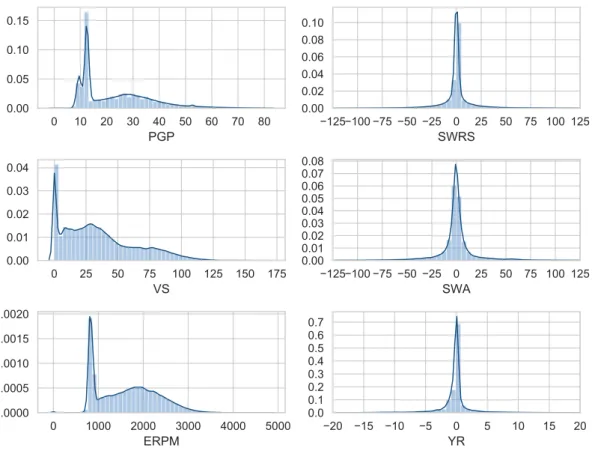
Figure 2.3 shows the histogram of some of the primary sensors from the CAN-bus. The percentage gas pedal (PGP) sensor readings range from 0 to 100, but the majority of readings are below 80. It does not follow a familiar distribution, and there is a peak around 10%, which is probably the sensor reading when the foot is resting on the pedal
or a gentle gas is applied to maintain the speed. The VS is measured in km h−1 and
ranges from0 km h−1 to 174 km h−1, speeds over 130 only happen once, probably one of
the participants got overexcited. There is a notable peak at 0, representing the vehicle at a halt, such as stopping at red-lights or waiting for the traffic to make turns. There
are at least two other peaks at around30 km h−1 and 76 km h−1, the former is probably
the average speed in streets and the latter the average speed in the highway. The engine
revolutions per minute (ERPM) is measured in revolutions per minute (rpm). This
signal is quite smooth, mainly because even though it is a function of driver depressing gas pedal, but since it is combined with gear shifting and filtered by the limitations of
0:00:00 0:16:40 0:33:20 0:50:00 1:06:40 1:23:20 Trip duration (H:M:S) IM1026 IM1028 IM1086 IM1067 IM1009 IM1087 IM1056 IM1049 IM1037 IM1052 IM1063 IM1022 IM1019 IM1057 IM1066 IM1058 IM1084 IF1013 IM1071 IM1047 IM1038 IF1011 IF1012 IM1062 IM1070 IM1033 IM1065 IM1041 IM1018 IM1046 IM1051 IM1048 IM1044 IM1027 IM1043 IM1050 IM1069 IF1017 IM1089 IM1072 IM1078 IM1061 IF1006 IF1019 IF1009 IM1085 IM1031 IM1079 IM1068 IM1059 IM1053 IM1045 IM1073 IM1034 IM1054 IM1035 IF1016 Driver ID
Figure 2.1: Trip lengths, the trips range from 33 minutes to 1 hour and a half. The
median trip duration is about 47 minutes. Trips with exceptionally long duration are due to traffic jams.
Figure 2.2: A trip from the Uyanik dataset. It consists of a 25 kmlong stretch. The
trip starts at the university (top right on the map), after a short ride in the university campus, a city traffic driving, motorway traffic, a dense city driving, ends back at the point of departure. 0 10 20 30 40 50 60 70 80 PGP 0.00 0.05 0.10 0.15 125 100 75 50 25 0 25 50 75 100 125 SWRS 0.00 0.02 0.04 0.06 0.08 0.10 0 25 50 75 100 125 150 175 VS 0.00 0.01 0.02 0.03 0.04 125 100 75 50 25 0 25 50 75 100 125 SWA 0.00 0.01 0.02 0.03 0.04 0.05 0.06 0.07 0.08 0 1000 2000 3000 4000 5000 ERPM 0.0000 0.0005 0.0010 0.0015 0.0020 20 15 10 5 0 5 10 15 20 YR 0.0 0.1 0.2 0.3 0.4 0.5 0.6 0.7
Figure 2.3: Histogram of main signals for all drivers - the dark blue line is drawn
using kernel density estimation with Gaussian kernel, it only serves as visualization purposes. Plots for SWRS, SWA, YR are trimmed as there are a few outliers much further than the currently depicted values.
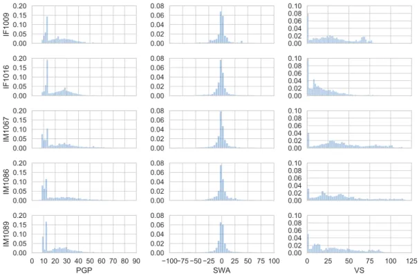
0.00 0.05 0.10 0.15 0.20 IF1009 0.00 0.02 0.04 0.06 0.08 0.00 0.02 0.04 0.06 0.08 0.10 0.00 0.05 0.10 0.15 0.20 IF1016 0.00 0.02 0.04 0.06 0.08 0.00 0.02 0.04 0.06 0.08 0.10 0.00 0.05 0.10 0.15 0.20 IM1067 0.00 0.02 0.04 0.06 0.08 0.00 0.02 0.04 0.06 0.08 0.10 0.00 0.05 0.10 0.15 0.20 IM1086 0.00 0.02 0.04 0.06 0.08 0.00 0.02 0.04 0.06 0.08 0.10 0 10 20 30 40 50 60 70 80 90 PGP 0.00 0.05 0.10 0.15 0.20 IM1089 100 75 50 25 0 25 50 75 100 SWA 0.00 0.02 0.04 0.06 0.08 0 25 50 75 100 125 VS 0.00 0.02 0.04 0.06 0.08 0.10
Figure 2.4: Histogram of PGP, SWA, VS for 5 drivers. To help comparison, x and y
axis are in the same range for all drivers. SWA is trimmed at -100 and +100 to improve visualization.
the engine, the result is more diluted and reflects less of the driver itself. There is a
peak at around 900rpm, which we suspect to be the idle engine rate. The other signals
presented in Figure 2.3 are steering wheel relative speed (SWRS), steering wheel angle (SWA), and yaw rate (YR). These signals have a Gaussian shape; however, these many
outliers are not expected in a Gaussian distribution. The SWA is in◦, and SWRS and
YR are measured in ◦s−1. The YR is slanted to the right and SWA to the left. This
pattern is because the route is followed in a counter-clockwise direction. Therefore the majority of turns are left-turns, lead to having more negative SWA values than positive. We see the opposite pattern in YR because left turns cause positive YR.
Figure 2.4 shows how different drivers express different histograms. The most significant differences are visible in PGP and VS. For example, we see that the first two drivers always keep some pressure on the pedal. However, the other three drivers have two modes at around 10%. One probably corresponds to the idle pedal state, which is close to 10% and another peak at around 13% (a gentle continuous pressure on the pedal). It is also possible to see that the spread varies between drivers. The SWA histograms look similar to each other. We notice that the first driver has a more spread out histogram than the fourth driver. There is a clear distinction between the VS histograms. For instance, the third and fourth drivers, drive faster, but with lots of variation at higher speeds. On the other hand, the first driver seems to be more cautious and drives at the
0 25 YR 500 0 SWA 250 0 250 SWRS 0 25 VS 25 50 75 PGP 0:00:50 0:01:40 0:02:30 0:03:20 0:04:10 0:05:00 0 2500 ERPM
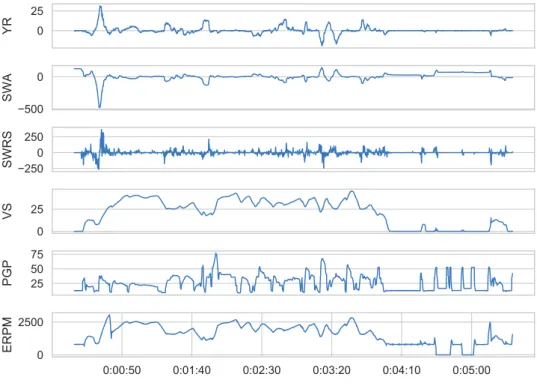
Figure 2.5: Example snapshot of raw sensor data for driver IM1048.
constant speed of around70 km h−1 in the highway. Another interesting example would
be the second driver, who is driving at lower speeds than the other drivers. One should be careful not to make judgments, only based on this histogram, because the very same driver could be a driver that usually drives much faster. However, in this recording, due to traffic conditions, they could not drive as fast as they usually would.
Figure 2.5 shows an example of raw CAN-bus data (IM1048), comprised of about 5 minutes from the beginning of the experiment. There are a few interesting things to notice in this figure. For instance, SWA and YR mirror each other. The SWRS also follows the SWA but appears to be noisy. We also notice a correlation between PGP and ERPM, which is expected. There is also a slight irregularity at about 4:30, in which ERPM drops to zero, it is likely that there is an issue, and the engine shuts off. However, since it can be seen that SWA is still following reasonable measurements, this is not a case of recording malfunction.
Distracted Driving Detection
Christopher Hitchens
3
Introduction to Distracted Driving Detection
N
OWADAYS, Internet-enabled smartphones have become ubiquitous, and we allwitness the flood of information that often arrives with a notification. We im-mediately divert our attention to our smartphones, even when we are behind the wheel. Statistics show that distraction-related crashes are on the rise [2]. A recent study shows that drivers use their phones in about 88% of their trips, an average of 3.5 minutes for each hour of driving [6].Mobile phone use increases the likelihood of a crash by fourfold [7]. Numerous other research points out the dangers of distraction for passenger safety [9]. Cell phone conversations significantly reduce reaction times and have other adverse effects [59, 60]. Moreover, contrary to popular belief, the use of hands-free devices is as detrimental as hand-held devices [59–61]. Although most distractions are due to smartphone use or conversations with passengers, manual or visual distractions are as essential and require attention [62].
For years distracted driving and its repercussions have been a known threat to passenger safety, and decision-makers have been trying to address this issue, these efforts rendered futile. Currently, 150 countries have national mobile phone laws in place, and 145 of them prohibit the use of hand-held mobile phones while driving. However, there is insufficient evidence on the effectiveness of legislation [1, pg. 45].
The most effective way of reducing distraction-related crashes is replacing the hu-man driver with a computer program. However, even though car companies are rac-ing to brrac-ing self-drivrac-ing cars to the markets, it will take decades until they become
widespread. A more reachable solution would be through advanced driver-assistance systems (ADASs), in which we have seen lots of progress. Unfortunately, such life-saving technologies are expensive, and the masses cannot afford them. Especially considering that developed countries only account for 7% of road traffic death, not even ADASs will have a significant impact on road safety at global levels.
3.1
State-of-the-art
Many attempts are made to formalize distracted driving, but there is no consensus.
Inattention is widely accepted as a major cause of unsafe driving and crash, Regan
et al. [63] define driver inattention as “insufficient or no attention to activities critical
for safe driving”. According to the latest driver inattention taxonomy from the United
States and EU Bilateral Intelligent Transportation Systems Task Force [64], drowsiness and distraction are two significant causes of inattention. According to Lee et al. [65]: “Driver distraction is a diversion of attention away from activities critical for safe driving toward a competing activity.” Distraction affects driving in various ways. Dong et al. [66] categorize them into three groups:
1. Driver Behavior Patterns - This category covers patterns of actions such as
rearview mirror checks or forward view inspection activities during driving. Drivers engaged in demanding cognitive tasks, lessen or some even abandon the visual monitor-ing of the mirrors or the instrument cluster Harbluk et al. [67]. More specifically, medium or heavy cognitive loads reduce the average area of the visual field to 92.2 and 84.41%, respectively [68]. These patterns are difficult to measure and, in most cases, require the use of intrusive sensors such as cameras.
2. Physiological Responses - Physiological indicators such as electroencephalogram
(EEG), electrocardiogram (ECG) signals, skin conductance, and blinking rate fit this category. It is shown that EEG workload increased with working memory load and problem-solving tasks [69]. Researchers demonstrate that visual and cognitive distraction leads to a temperature increase on the skin surface [70]. The main issue with such metrics is the need for sophisticated sensors that are also uncomfortable or intrusive.
3. Driving Performance - Maintaining speed and lane-keeping are two examples of
driving performance metrics that are affected by distractions. Zhou et al. [71] show that performing secondary tasks influence checking behavior (e.g., mirror checking) both in frequency and duration, which leads to a lower rate of lane changing. In this example,
the decline in driving performance is a symptom of a change indriver behavior patterns—
which falls in the first category. Liang and Lee [72] establish that cognitive distraction causes intermittent steering. Steering neglect and over-compensation are associated with visual distraction and under-compensation with cognitive distraction. Although sophis-ticated sensors are required to measure metrics such as headway distance—requiring
radar, available in cars equipped with adaptive cruise control (ACC)—or lane-changing behavior—requiring road facing cameras, available in cars equipped with LKA—such sensors are not intrusive towards the driver and are becoming more prevalent in the high-end vehicles.
The distracted driving literature has focused only on one or a hybrid of the cat-egories mentioned above. However, most of the studies take one of the first two
ap-proaches, driver behavior patterns or physiological responses; we suspect because these
approaches fit better in already established fields of medical and behavioral psychology research. Besides, such metrics are already well defined and perceived to be more reliable for distraction detection.
There is a large body of research that shows nomadic devices such as smartphones can be used for driver profiling and to detect unsafe driving. These works mainly use indicators such as harsh cornering or acceleration that can be obtained from smartphone
sensors1. Only a few of these works focus on distraction detection. It is essential not
to confuse unsafe driving with distracted driving, even though sometimes they manifest similar symptoms (such as harsh braking). Distracted driving is unsafe, but unsafe driving does not always constitute distracted driving. There are a number of ways that smartphones can be used to detect distraction. For instance, You et al. [74] use dual cameras on smartphones to detect drowsy and distracted driving. Bo et al. [75] use the magnetometer and the accelerometer from a smartphone to detect texting while driving. Lastly, Jiang et al. [76] show that wrist-worn smart devices can be used to detect distracted driving.
Next, we present examples of distracted driving detection methods that are relevant to our work. Wöllmer et al. [30] proposed to use head orientation to detect distractions, which mainly consists of user interactions with the instrument cluster. Additionally, they also use some of the vehicle operation signals such as pedal and steering wheel data as well as some driving performance metrics such as deviation from the center of the traffic lane and heading angle [30]. This rich set of signals were used as input to a long short-term memory (LSTM) recurrent neural network, which results in a subject-independent detection of distraction with up to 96.6% accuracy.
In a more relevant study, Jin et al. [77] develop two models based on support vector machine (SVM) called NLModel and NHModel, which are designed to detect low and high cognitive distractions, respectively. In this work, they only use data from the vehicle’s internal network (CAN-bus) as input. Signals include vehicle operation parameters as well as vehicle dynamics. They achieve an accuracy of about 73.8% and a sensitivity of approximately 61.8%.
In another study, Tango and Botta [31] propose a subject dependent model based on SVM that can achieve accuracy of up to 95%. They only use the dynamic signals of the vehicle for classification; however, data annotation is done accurately with the help of eye-tracking cameras and human supervision. The experiments are performed
in a mostly straight highway drive and at the speeds of around100 km h−1. Such
over-simplifications raise questions regarding the robustness and reliability of the model in real-world environments.
Lastly, Öztürk and Erzin [78] propose the use of GMM for distraction detection. They extract cepstral features from the pressure on Gas and Brake pedals. Using GMM as
a classifier and a decision window of length360 s, they achieve 93.2% success to recognize
non-distracted driving and 72.5% success in recognizing distracted driving [78].
In the next chapter, we propose a distracted driving detection mechanism that can detect distractions and warn the driver and, at the same time, be accessible to a considerable portion of car owners. Although this work is not the first attempt at solving this problem, it follows a novel and ambitious approach. Current literature mostly uses sophisticated sensors to detect distractions, sensors such as cameras for tracking head orientation [30] or measuring the skin temperature [70]. However, we propose to use the standard vehicle sensors; therefore, this method could apply to vehicles on the market.
Rumi
4
Non-Intrusive Distracted Driving Detection
Based on Driving Data
In this chapter, we present a distracted driving detection approach that does not use any intrusive sensors, such as cameras or microphones; instead, we focus on driving data. We aim to classify driving segments as distracted or not distracted driving. Such a system can be used on-line to alert the driver in case of continuous distraction or off-line as a metric to judge the driving performance or asses riskiness.
First, we use a sliding window (frame) to extract features from driving signals, then using ML, we classify each window as distracted or not-distracted, then a decision function decides whether a sequence of frames represents distracted driving or not. We propose to validate this method using driving traces from 13 drivers chosen from a large driving Uyanik dataset [51] (see Chapter 2). For evaluation, we present the performance
of the proposed method in terms of F1 score and area under the receiver operating
characteristic (ROC AUC). The remainder of the chapter is organized as follows, in Section 4.1, we describe the proposed methodology and the evaluation strategy. In Section 4.3, we present the evaluation results, and in Section 4.4, we discuss the obtained results. Lastly, in Section 4.5, we summarize and present future directions.
Driving Signals Low Pass Filter Add 1st order derivatives Windowing Function PGP SWA All Signals Extract Statistical Features Extract Cepstral Features Classifier hw Decision Function fMVor fMS Output ˆ y
Figure 4.1: Distraction Detection Process
4.1
Methodology
We formulate the problem as a supervised learning problem. In which the input data is a multivariate time series recorded from a vehicle, and the target is 0 for normal driving
and 1 for distracted driving. We denote a driving trace as (x(i), y(i))Ni=1, wherex is the
sensor measurements from the car, y ∈ {0,1} is the target label, and N indicates the
total number of measurements. We seek a function h that predicts yˆ for short driving
sequences. Sincex is a multivariate sequence, it is not possible to apply classic machine
learning algorithms; therefore, we use the sliding window approach in order to apply
conventional ML algorithms [79]. We use window classifier hw to map each window
frame of length w into individual predictions. Let d = (w−1)/2 be the half-width
length of the window, for a window frame at time t, hw makes prediction yˆt based
on window frame hxt−d, . . . , xt, . . . , xt+di. To reduce the computational complexity, we
make window predictions for everyk=bw∗(1−100r )csamples, wherekdenotestep size
andr indicates the percentage of overlap between two consecutive window frames. This
results in M = Nk window frames. Since it is possible that a window frame cover both
distracted and non-distracted measurements, we label a window frame as distracted only
if more than 50% of the measurements are distracted. Each driving trace(x(i), y(i))Ni=1 is
converted intoM window frames, thenhw is trained using feature vectorsxcomputed for
each window frame and its corresponding label. Similarly to classify an unseen driving
trace x, it is first converted into window frames, then for each window frame at time t
feature vectorxtis computed andhw makes the predictionyˆtbased onx. Lastly, we feed
lconsecutive window frame predictions (hytˆ−l,ytˆ−l+1, . . . ,ytˆi) to the decision functionf
which produces the final prediction for the given sequence.
4.1.1 Evaluation Method
In order to utilize the entire driving tracesD={(xi, yi)}Ki=1for both training and testing,
we employ a K fold cross-validation method called leave-one-group-out. Each time we
train a model using data from K −1 drivers and validate that on the data from the
remaining driver. In other words, each driver is considered a group; therefore, at each
on its prediction performance over the remaining slice. This is a subject-independent model because the model has no information about the driver that is being tested on. We evaluate the proposed mechanism using data from 13 drivers; therefore, in this case, K = 13.
Drivers typically drive attentively, but sometimes they get distracted by engaging in secondary tasks. We see the same pattern in our dataset; on average, only 36% of the measurements are labeled as distracted. Since the dataset is imbalanced in order to have
a better measure of the proposed model’s performance, we choose to report F1 score as
well as ROC AUC as the primary performance metrics. F1 score is the harmonic mean
of precision and recall:
F1 = 2· 1 1 recall+ 1 precision (4.1) Since our classification problem is binary, based on the application needs, we can modify the decision threshold. In order to avoid introducing new parameters, we employ the receiver operating characteristic (ROC), which demonstrates the diagnostic ability of a binary classifier as its discrimination threshold is varied. In fact, we use ROC AUC, which is a simple way of reporting an ROC plot using one numeric value (area under the ROC curve).
4.2
Video Annotation and Synchronization with Sensors
This section describes how we hand-annotate the distractions in a subset of the Uyanik
dataset. It consists of two partsa) data annotationb) synchronization. The participants
of the Uyanik data collection perform secondary tasks during the trip. By watching the videos from the driver-facing camera, we can mark the times the driver is engaged in these secondary tasks, which we use as a proxy for being distracted.
From the drivers with valid CAN and IMU data, we select the ones with available driver-facing video. We watched the videos and noticed that not all of them follow the same protocol. Several drivers skip some secondary tasks, or the tasks they perform are very different. This is particularly challenging because the conversations are in Turkish. Since we do not speak Turkish, based on their similarity, we had to decide if they follow the same protocol. The annotation consists of marking the beginning and end of each secondary task.
Having the timestamps of the secondary tasks on the video is not enough because the videos are not synchronized with the sensor data. To tackle the synchronization issue, we took inspiration from a work by Fridman et al. [80]. The general idea is that in a moving vehicle, turning the steering wheel results in lateral movements of the car. These lateral movements are visible in the front-facing camera feed, and they should correlate with steering wheel movements. Therefore if we find the time lag that maximizes the
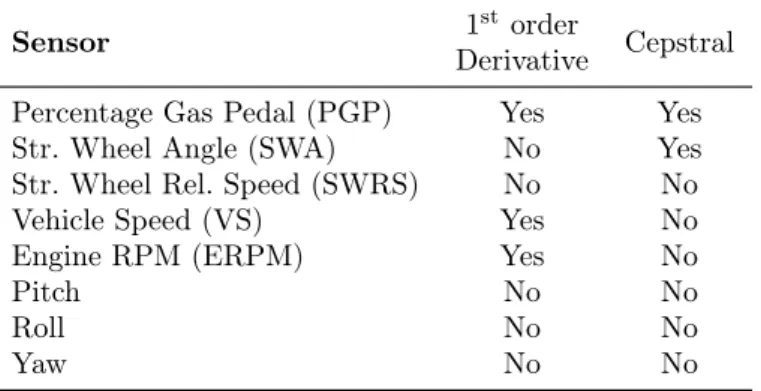
Table 4.1: Selected Signals for Driver Distraction Detection
Sensor 1
st order
Cepstral Derivative
Percentage Gas Pedal (PGP) Yes Yes
Str. Wheel Angle (SWA) No Yes
Str. Wheel Rel. Speed (SWRS) No No
Vehicle Speed (VS) Yes No
Engine RPM (ERPM) Yes No
Pitch No No
Roll No No
Yaw No No
cross-correlation between the two signals, we can use it to synchronize the videos with the other sensor data. To achieve this goal, first, we use the front-facing video feed to estimate the vehicle’s lateral movements. A dense optical flow method based on Gunner Farneback’s algorithm [81] is then applied to the video. The result is a two-channel array representing the optical flow vectors. These vectors point to the direction of the movement of image pixels. We take the average of the horizontal component of all pixels and maximize its cross-correlation with the SWA. This method produces satisfying results for the majority of the recordings. In this work, we annotate and synchronize data from 13 drivers, composed of 2 female and 11 male drivers.
4.2.1 Feature Extraction
In order to remove high-frequency noise, we apply a low pass filter to all the signals to smoothen the signals. Then for some of the signals (Shown in Table 4.1) we derive the temporal derivative of the signals. For both smoothing and computation of derivations, we use an implementation of the Savitzky-Golay algorithm [82]. Figure 4.1 shows the various stages that the signals go through before the feature extraction step. In this study, we use eight signals, which are listed in Table 4.1. These signals are obtained from CAN-bus or IMU. Then we apply a windowing function to all the signals, which takes two
parameters,wto determine the length of the frame andrto specify the amount of overlap
between the two consecutive frames. This will break down the signal into frames of sizew
and is ready for the feature extraction stage. Per each signal, nine statistical features are extracted from each frame. These descriptive statistics are selected to be representative of the distribution of sensor values covered by the frame. This set includes minimum, maximum, mean, median, standard deviation, kurtosis, skewness, and the number of zero crossings. We also extract cepstral features from two signals, PGP and SWA, these are the only vehicle operating inputs that are directly operated by the driver. Earlier studies have shown that cepstral analysis is suitable for driver identification [35, 54], we suspect that they are also useful for detecting distracted driving.
The implementation is as follows; we multiply a Hamming window of lengthwto
limit the signal and also reduce the edge effects. We denotec(k)to be the firstkcepstral
coefficients, and higher-order coefficients are discarded. The equation to derive c(k) is:
c(k) =F−1{log(|F {xtwt}|)}
(4.2)
Wherextdenotes signal values covered by the current frame, wt denote Hamming
win-dow with the same length as the frame and F, and F−1 denote discrete Fourier
trans-form (DFT) and inverse-DFT (IDFT) respectively. We extract cepstral features from
two signals, PGP and SWA, and keep the firstk= 32coefficients as cepstral features.
Table 4.2: Average Scores For Each Signal
Signal Mutual Info. F-Test
SWRS 0.517 0.084 ERPM Derivative 0.510 0.059 Pitch 0.490 0.056 PGP Derivative 0.475 0.035 Roll 0.470 0.012 PGP 0.436 0.060 ERPM 0.428 0.359 VS Derivative 0.427 0.088 Yaw 0.425 0.054 VS 0.415 0.792 SWA 0.228 0.061 Cepstral Coefficients PGP 0.029 0.036 Cepstral Coefficients SWA 0.025 0.026
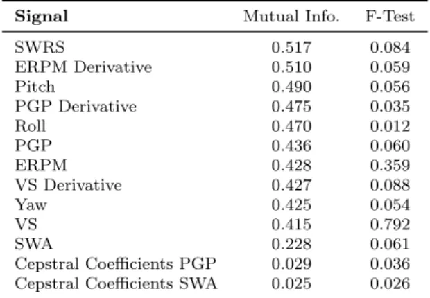
4.2.2 Feature Importance
We analyze the extracted features to evaluate their fitness for our experiments. We use two metrics for this purpose, the conventional ANOVA F-test and mutual informa-tion (MI) [83, 84] as two metrics to evaluate the importance of the features as well as some insights into which features or signals are more important for our classification task. To get an idea that which signal is more important, first we compute the MI for all features, we normalize it and compute the average importance for five best features from each signal. Since we compute nine features for each signal, it is unrealistic to expect all the features from a signal to be equally informative. Therefore we choose a number of the best features per signal (in this case, 5) as a proxy for the importance of the signal. The corresponding results are presented in Table 4.2. Since the methods based on F-test only estimate the linear dependencies while MI captures linear and non-linear dependencies, we sort the signals in descending order of their MI score. Among the signals, we can observe that features extracted from SWRS have the highest MI score, and the cepstral features are the worst.
We perform a similar analysis to assess which functions used for feature extraction are the most informative. The corresponding results are presented in Table 4.3. We can
Table 4.3: Average Scores For Each Function Function Mutual Info. F-Test
Min 0.955 0.310 Max 0.933 0.289 Range 0.495 0.076 Median 0.136 0.309 Mean 0.092 0.314 Standard Deviation 0.053 0.067 # Zero crossings 0.040 0.166 Cepstral Coefficients 0.034 0.039 Skewness 0.032 0.041 Kurtosis 0.030 0.081
see that simple functions such as Min, Max, Range, Mean are more useful that Skewness and Kurtosis.
4.2.3 Classification Algorithms
We select five classification algorithms to be used as frame classifier hw. The following
is the list of classifiers used in this study along with their corresponding parameters.
AdaBoost (AB). AdaBoost, as introduced by Freund and Schapire [85], suggests the use
of a collection of weak learners. As the number of weak learners increases, the algorithm increases the weight for examples that are more difficult (are currently misclassified), therefore improving the performance. We use the implementation from the scikit-learn library [86], which uses the AdaBoost-SAMME algorithm [87]. We use a decision tree with a maximum depth of 1 as weak learner [88]. Two hundred decision trees as a weak learners, learning rate = 0.75.
Gradient Boosting (GB). Gradient boosting, iteratively combines weak learners into
a single strong learner. At each iteration, GB fits a tree to correct the mistakes of the model from previous iteration. Therefore in principle, Gradient boosting fits models to the residuals of the previous iteration. These residuals are equivalent to the negative of the gradients [89]. 100 estimators, maximum depth = 6, maximum features = None, maximum depth = 6, learning rate = 0.05.
Random Forest (RF). Random Forests were introduced by Breiman [90]. As the
name suggests, it consists of a combination of tree predictors. Each tree is trained on a subsample of the examples, which is also known as bagging. Moreover, to further reduce the correlation between the trees and avoid overfitting, each tree is fitted on a subset of features. We use the implementation from scikit-learn package [86]. With parameters: 200 estimators, maximum features = None, maximum depth = 7, class weight = balanced.
Support Vector Machine (SVM). Lastly, we step away from tree-based algorithms
and attend to once upon a time king of classifiers, SVM. SVMs for some time were known to be the best classifiers available. Vladimir Vapnik introduced the linear support-vector
machines in 1965. SVMs are binary classifiers, in linear case SVM finds the maximum-margin hyperplane that separates the two class. Cortes and Vapnik [91] in 1995 proposed to use the kernel trick [92] and extended SVM to solve non-linear classification problems. In this approach instead of dot products in SVM a non-linear kernel function is used. Therefore the algorithm is able to fit maximum-margin hyperplane in a transformed space, which allows for separation of non-linear feature boundaries. We use the SVC classifier from scikit-lean library [86] which uses LIBSVM library [93]. RBF kernel, C =
0.1, γ = 0.01, class weight = balanced.
k-Nearest Neighbors (k-NN) k-nearest neighbors (k-NN) in order to classify an
un-labeled example finds thekclosest examples in the training set and selects the majority
class. # neighbors = 5.
In our experiments, we use the implementations from the scikit-learn software package. All other parameters are set to their default values as of scikit-learn version 0.19.2 [86].
4.2.4 Decision Functions
The decision function f determines the final prediction yˆ at time t based on the last
l frame predictions, we call this a decision window: hyˆt−l, . . . ,yˆt−1,yˆti, therefore l is
the number of frames covered by a decision window. Below we introduce two decision
functions to obtain yˆand evaluate their performance later in Section 4.3:
1) Majority vote (MV) Letd to denote count of the frames in the decision window
that are predicted as distracted driving. Then a decision window is classified as distracted
if d
l >0.5.
2) Maximum score (MS) Let d0 to be the cumulative classification score for the
distracted class. Then a decision window is classified as distracted if d0
l >0.5.
4.3
Model Performance
In this section, we present the results of our experiments. In each subsection, we focus on one of the components of our proposed methodology and discuss its implications.
4.3.1 Frame-size Analysis
In order to find out the optimal frame-size, we try several sizes1 as well as overlap ratios2.
Since we do not want to have results influenced by choice and working mechanism of the
decision function, in these experiments, we do not apply the decision function f and
only consider the predictions from hw. The results are presented in Figure 4.2, the
reported numbers are the average cross-validated scores for each combination ofr andw
1
Frame-sizes of 4, 7, 10, 15, 20, 30, 45 and 60 2
0 25 50 75 90 Frame overlap (%) 4 7 10 15 20 30 45 60 Frame-size (seconds) 0.672 0.673 0.680 0.678 0.682 0.673 0.676 0.685 0.686 0.692 0.685 0.674 0.688 0.697 0.700 0.672 0.693 0.704 0.709 0.706 0.697 0.702 0.717 0.721 0.719 0.695 0.720 0.737 0.740 0.739 0.728 0.725 0.743 0.769 0.758 0.723 0.739 0.761 0.764 0.764 F1 Score 0.68 0.70 0.72 0.74 0.76 0 25 50 75 90 Frame overlap (%) 4 7 10 15 20 30 45 60 Frame-size (seconds) 0.741 0.740 0.746 0.746 0.750 0.742 0.747 0.759 0.763 0.766 0.756 0.747 0.767 0.774 0.776 0.752 0.768 0.783 0.787 0.788 0.765 0.782 0.789 0.801 0.802 0.769 0.803 0.812 0.811 0.820 0.802 0.791 0.814 0.838 0.841 0.775 0.800 0.829 0.841 0.847
ROC AUC Score
0.74 0.76 0.78 0.80 0.82 0.84
Figure 4.2: The effect of frame-size on classification score. BothF1 and ROC AUC
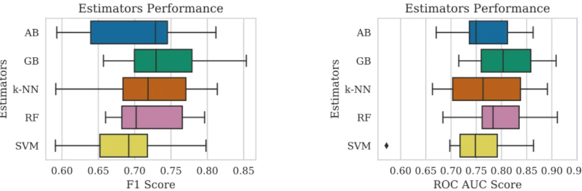
follow a similar pattern. Incr